Community Structures Are Definable in Networks: A Structural Theory of Networks

State Key Laboratory of Computer Science, Institute of Software, Chinese Academy of Sciences, P. O. Box 8718, Beijing, 100190, P. R. China. Email: {angsheng, yicheng, lijk}@ios.ac.cn. Correspondence: {angsheng, yicheng}@ios.ac.cn.
Angsheng Li is partially supported by the Hundred-Talent Program of the Chinese Academy of Sciences. All authors are supported by the Grand Project “Network Algorithms and Digital Information” of the Institute of software, Chinese Academy of Sciences, and NSFC grant No. 61161130530.

Angsheng Li Affiliation: State Key Laboratory of Computer Science Institute of Software, Chinese Academy of Sciences Yicheng Pan Affiliation: State Key Laboratory of Computer Science Institute of Software, Chinese Academy of Sciences Affiliation: State Key Laboratory of Information Security Institute of Information Engineering, Chinese Academy of Sciences, P. R. China Jiankou Li Affiliation: State Key Laboratory of Computer Science Institute of Software, Chinese Academy of Sciences Affiliation: University of Chinese Academy of Sciences, P. R. China

Community detecting is one of the main approaches to understanding network structures. However it has been a longstanding challenge to give a definition for community structures of networks. We found that neither randomness in the ER model nor the preferential attachment in the PA model is the mechanism of community structures of networks, that community structures are universal in real networks, that community structures are definable in networks, that communities are interpretable in networks, and that homophyly is the mechanism of community structures and a structural theory of networks. We proposed the notions of entropy- and conductance-community structures. It was shown that the two definitions of the entropy- and conductance-community structures and the notion of modularity proposed by physicists are all equivalent in defining community structures of networks, that neither randomness in the ER model nor preferential attachment in the PA model is the mechanism of community structures of networks, that there is an empirical criterion for deciding the existence and quality of community structures in networks, and that the existence of community structures is a universal phenomenon in real networks. This poses a fundamental question: What are the mechanisms of community structures of real networks? To answer this question, we proposed a homophyly model of networks. It was shown that networks of our model satisfy a series of new topological, probabilistic and combinatorial principles, including a fundamental principle, a community structure principle, a degree priority principle, a widths principle, an inclusion and infection principle, a king node principle and a predicting principle etc. The new principles provide a firm foundation for a structural theory of networks. Our homophyly model demonstrates that homophyly is the underlying mechanism of community structures of networks, that nodes of the same community share common features, that power law and small world property are never obstacles of the existence of community structures in networks, that community structures are definable in networks, and that (natural) communities are interpretable. Our theory provides a foundation for analyzing the properties and roles of community structures in robustness, security, stability, evolutionary games, predicting and controlling of networks.

1 Background

Defining community structures in networks is a fundamental challenge in modern network theory. Our notions of the entropy- and conductance-community structures are information theoretical and mathematical definitions respectively. We found that our definitions of entropy-, conductance- and the modularity-community structures [18] are equivalent in defining community structures of networks, that randomness and preferential attachment are not mechanisms of community structures of networks, and that community structures are universal in real networks. This shows that community structure is a phenomenon definable in networks. The discoveries here provide a foundation for a new theory of community (or local) structures of networks.

Generally speaking, the missing of a structural theory of networks hinders us from rigorous analysis of networks and networking data. In fact, the current state of the art shows that the current tools for analyzing networks and networking data are mainly the probabilistic or statistical methods, which of course neglect the structures of data.

However, structures are essential. In nature and society, especially in the current highly connected world, we observe that mechanisms determine the structures, and that structures determine the properties, which could be a new hypothesis of real network data. In particular, a grand challenge in network science is apparently the missing of a structural theory of networks. Community structures determine the local properties of networks that may have global implications.

Network has become a universal topology in science, industry, nature and society. Most real networks satisfy a power law degree distribution [3], [2], and a small world phenomenon [17], [23], [13].

Community detecting or clustering is a powerful tool for understanding the structures of networks, which has already been extensively studied [5], [8], [21], [9], [19]. Many definitions of communities have been introduced, and various methods for detecting communities have been developed in the literature, see [12] for a recent survey. However, the problem is still very hard, not yet satisfactorily solved. The approach of community finding takes for granted that networks have community structures. The fundamental questions are thus: Are communities objects naturally formed in a network or simply outputs of a graphic algorithm? Can we really take for granted that networks have community structures? Are community structures of networks robust? What are the natural mechanisms which generate the community structure of a network, if any? What can we do with the communities? How can we test the quality of various community finding algorithms?

Our experiments here showed that community structures are definable in networks, that randomness and preferential attachment are not mechanisms of community structures of networks, that there is an empirical criterion for deciding the existence and quality of community structures of networks, and that the existence of community structures is a universal phenomenon of real world networks. This predicts that community structures have their own mechanisms other than the well-known ones of classical models of networks.

It is easy to recognize that the key to answer all the questions listed above is to understand the mechanisms of community structures of networks.

We proposed a new model of networks, the homophyly model below, by introducing the new mechanism of homophyly in the classical preferential attachment model. Our model constructs networks dynamically by using the natural mechanisms of preferential attachment and homophyly.

Our homophyly model explores that homophyly is the mechanism of community structures in networks, that community structures are provably definable in networks, and that communities are interpretable in networks. It was shown that the homophyly networks satisfy simultaneously a series of new topological, probabilistic and combinatorial principles, including a fundamental principle, a community structure principle, a degree priority principle, a widths principle, an inclusion and infection principle, a king node principle and a predicting principle etc. The new principles we found here provide a foundation for analyzing the properties and roles of community structures in new issues of networks such as robustness, security, stability of networks, evolutionary game and predicting in networks, and controlling of networks. Our results here provide a firm first step for us to develop a structural theory of networks, which would be essential to many important new issues of networks and networking data.

2 Definitions of Community Structures of Networks

The first definition of community structures is the notion of modularity. Newman and Girvan [18] defined the notion of modularity to quantitatively measure the quality of community structure of a network. It is built based on the assumptions that random graphs are not expected to have community structure and that a network has a community structure, if it is far from random graphs.

Let $G=(V,E)$ be a graph with $n$ nodes and $m$ edges and $\mathcal{P}$ be a partition of nodes in $V$ . The modularity of $G$ by $\mathcal{P}$ is defined by

\sigma^{\mathcal{P}}(G)=\frac{1}{2m}\sum\limits_{i,j}(A_{ij}-P_{ij})\delta(C_{i},C_{j}),

where the sum runs over all pairs of vertices, $A$ is the adjacency matrix, $P_{ij}$ is the expected number of edges between nodes $i$ and $j$ in a null graph, i.e., a random version of $G$ . $\delta(C_{j},C_{j})=1$ if $C_{i}=C_{j}$ , and $0$ otherwise, $C_{k}$ is an element of the partition $\mathcal{P}$ .

A standard null model imposes that the expected degree after averaging over all possible configurations matches the actual degree of the original graph [11]. Such a null model is essentially equivalent to the configuration model [7], in which each node $i$ is associated with $d_{i}$ half-edges, where $d_{i}$ is the degree of node $i$ in $G$ , and all the half-edges are joined randomly. It is easy to obtain that $P_{ij}=d_{i}d_{j}/2m$ and the modularity of $G$ by $\mathcal{P}$ can then be rewritten as

\sigma^{\mathcal{P}}(G)=\sum\limits_{l=1}^{L}\left[\frac{k_{l}}{m}-\left(\frac{V_{l}}{2m}\right)^{2}\right],

(1)

where $L$ is the number of modules in partition $\mathcal{P}$ , $k_{l}$ is the number of edges whose both ends are in module $l$ , and $V_{l}$ is the sum of the degrees of the nodes in $l$ , also called the volume of $l$ . Note that the first term of each summation represents the fraction of edges of $G$ inside the module and the second term represents the expected fraction of edges that would be in the null model.

We define the modularity of $G$ as

\sigma(G)=\max_{\mathcal{P}}\{\sigma^{\mathcal{P}}(G)\}.

$\sigma(G)$ is a real number in $[0,1]$ . The larger $\sigma(G)$ is, the better community structure $G$ has. We define the modularity community structure ratio (M-community structure ratio) of $G$ to be the modularity of $G$ .

The second definition is based on random walks. The intuition is that random walks from a node in a quality community are not easy to go out of the community. We define the notion of entropy community structure ratio of a network. We consider the entropy of a network and of a network given by a partition of nodes of the network.

Let $G=(V,E)$ be a graph with $n$ nodes and $m$ edges, and $\mathcal{P}$ be a partition of $V$ . We use $L^{U}(G)$ to denote the minimum average number of bits to represent a single step of random walk (in the stationary distribution) with a uniform code in $G$ , and $L^{\mathcal{P}}(G)$ to denote the minimum average number of bits to represent that with an aforementioned “module-node” code.

By information theoretical principle,

L^{U}(G)=-\sum\limits_{i=1}^{n}\frac{d_{i}}{2m}\cdot\log_{2}\frac{d_{i}}{2m},

(2)

where $d_{i}$ is the degree of node $i$ .

L^{\mathcal{P}}(G)=-\sum\limits_{j=1}^{L}\sum\limits_{i=1}^{n_{j}}\frac{d_{i}^{(j)}}{2m}\cdot\log_{2}\frac{d_{i}^{(j)}}{V_{j}}-\frac{m_{g}}{m}\left(\sum\limits_{j=1}^{L}\frac{V_{j}}{2m}\cdot\log_{2}\frac{V_{j}}{2m}\right),

(3)

where $L$ is the number of modules in partition $\mathcal{P}$ , $n_{j}$ is the number of nodes in module $j$ , $d_{i}^{(j)}$ is the degree of node $i$ in module $j$ , $V_{j}$ is the volume of module $j$ , and $m_{g}$ is the number of edges crossing two different modules.

We define the entropy community structure ratio of $G$ by $\mathcal{P}$ by

\tau^{\mathcal{P}}(G)=1-\frac{L^{\mathcal{P}}(G)}{L^{U}(G)}.

We define the entropy community structure ratio of $G$ (E-community structure ratio of $G$ ) by

\tau(G)=\max_{\mathcal{P}}\{\tau^{\mathcal{P}}(G)\}.

We notice that similar idea has been used in community detecting, for instance, Rosvall and Bergstrom [22] proposed an algorithm to detect communities by compressing a description of the information flow by using the Huffman code to encode prefix-freely each module and each node. Our definition here is purely an information theoretical notion.

Both definitions of the modularity and entropy community structure ratio depend on partitions of $G$ . In these definitions, the existence of a community structure of a graph means that there is a “good partition” for the graph. However the intuitive relationship between “good partitions” and community structures is not clear, and more seriously, both the two definitions are not convenient for us to compare the community finding algorithms, which usually do not give partitions of networks. In fact, a community finding algorithm may find overlapping communities, and may neglect part of the nodes in the community findings. In addition, both modularity and the entropy community structure ratio can be regarded as global definitions of community structures of networks.

We will introduce a mathematical definition based on conductance, which is applicable to overlapping communities, and to partial solutions of searching etc. We define the conductance community structure ratio of a network. To describe our definition, we recall the notion of conductance.

Given a graph $G=(V,E)$ , and a set $S\subset V$ , the conductance of $S$ in $G$ is defined by

\Phi^{G}(S)=\frac{|E(S,\bar{S})|}{\min\{{\rm vol}(S),{\rm vol}(\bar{S})\}},

where $\bar{S}$ is the complement of $S$ in $G$ , $E(S,\bar{S})$ is the set of all edges with one endpoint in $S$ and the other in $\bar{S}$ , ${\rm vol}(X)$ is the volume of $X$ .

Clearly, a community of a network must satisfy certain basic conditions, for instance: the induced subgraph must be connected, and the size of the community is not too small, and not too large. For this, we define:

Definition 2.1

(Possible community) Given a graph $G=(V,E)$ , let $n=|V|$ , and $S\subset V$ . We say that $S$ is a possible community of $G$ , if:

(1)

The induced subgraph $G_{S}$ of $S$ in $G$ is connected,
(2)

$|S|\geq\log n$ , i.e., the size of $S$ is not too small, and
(3)

$|S|\leq\sqrt{n}$ , that is, the size of $S$ is not too large.

Definition 2.2

(Conductance community structure ratio of communities) Let $G=(V,E)$ be a graph, and $n=|V|$ . Suppose that $\mathcal{X}=\{X_{1},X_{2},\cdots,X_{l}\}$ is a set of possible communities of $G$ (overlapping is permitted). Then,

(1)

Let $X=\cup_{j}X_{j}$ .
(2)

For each $x\in X$ , suppose that $X_{j_{1}},X_{j_{2}},\cdots,X_{j_{r}}$ are all the possible communities $X_{j}\in\mathcal{X}$ that contain $x$ , then define

$a^{\mathcal{X}}(x)=\sum\limits_{i}^{r}(1-\Phi(X_{j_{i}}))/r.$
(3)

Define the conductance community structure ratio of $G$ by $\mathcal{X}$ by

$\theta^{\mathcal{X}}(G)=\frac{1}{n}\cdot\sum\limits_{x\in X}a^{\mathcal{X}}(x).$

By using $\theta^{\mathcal{X}}(G)$ , we define the conductance community structure ratio of a network.

Definition 2.3

(Defining $\theta(G)$ ) Let $G=(V,E)$ be a network. We define the conductance community structure ratio of $G$ by

\theta(G)=\max_{\mathcal{X}}\{\theta^{\mathcal{X}}(G)\}.

The conductance community structure ratio (C-community structure ratio, for short) can be interpreted as a mathematical definition of community structures of networks. It is a local definition of community structures of networks.

Suppose that $G=(V,E)$ is an expander with the following properties: for any nontrivial set $S\subset V$ , the conductance $\Phi(S)>\alpha$ for some large constant $\alpha$ . Then by definition, $\theta(G)<1-\alpha$ . Therefore $\theta(G)$ cannot be large for graph $G$ with expanding property. In particular, for a nontrivial network $G$ constructed from the PA model, with probability $1-o(1)$ , $\theta(G)<1-\alpha$ for some large constant $\alpha$ .

More importantly, the conductance community structure ratio can be defined for algorithms.

Definition 2.4

(Defining $\theta^{\mathcal{A}}(G)$ ) Let $G=(V,E)$ be a network. Let $\mathcal{A}$ be a community detecting algorithm. Suppose that $\mathcal{X}$ is the set of all possible communities of $G$ found by algorithm $\mathcal{A}$ . Then define:

\theta^{\mathcal{A}}(G)=\theta^{\mathcal{X}}(G).

By using Definition 2.4, we can define a community finding problem as follows.

Definition 2.5

(Community finding problem) To design an algorithm, $\mathcal{A}$ say, such that for any network $G$ , $\theta^{\mathcal{A}}(G)$ is maximized.

This gives rise to the algorithmic problem of searching.

3 Community Structures Are Robust

Now we have three definitions of community structure ratios of networks. Are there any relationships among the three definitions for the quality of community structures of networks, i.e., the M-, E-, and C-community structure ratios? Do the three definitions give the same answer to the question whether or not a network has a community structure? We conjecture that the answer is yes. For this, we propose the following:

Community structure hypothesis: Given a network $G$ , the following properties are equivalent,

1)

$G$ has an M-community structure,
2)

$G$ has an E-community structure, and
3)

$G$ has a C-community structure.

We verify the community structure hypothesis by computing the M-, E-, and C-community structure ratios for networks of classical models. The first model is the ER model [10]. In this model, we construct graph as follows: Given $n$ nodes $1,2,\cdots,n$ , and a number $p$ , for any pair $i,j$ of nodes $i$ and $j$ , we create an edge $(i,j)$ with probability $p$ . The second is the PA model [3]. In this model, we construct a network by steps as follows: At step $0$ , choose an initial graph $G_{0}$ . At step $t>0$ , we create a new node, $v$ say, and create $d$ edges from $v$ to nodes in $G_{t-1}$ , chosen with probability proportional to the degrees of nodes in $G_{t-1}$ , where $G_{t-1}$ is the graph constructed at the end of step $t-1$ , and $d$ is a natural number.

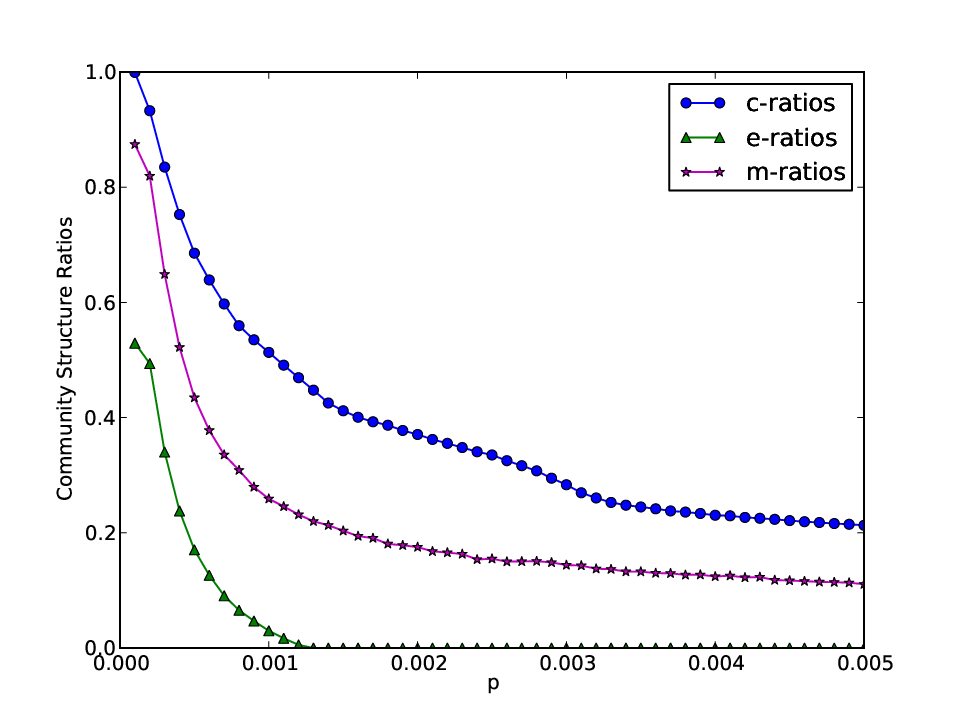
Refer to caption — Figure 1: This figure gives the E-, M- and C-community structure ratios (denoted by e-, m- and c-ratios respectively) of networks, for $n=10,000$ , and for $p$ up to $0.005$ of the ER model.

We depict the curves of the M-, E-, and C-community structure ratios of networks of the ER model and the PA model in Figures 1 and 2 respectively.

From Figures 1 and 2, we observe that the following results hold:

(1)

The curves of the M-, E-, and C-community structure ratios of networks generated from the ER model are similar.
(2)

The curves of the M-, E-, and C-community structure ratios of networks generated from the PA model are similar.
(3)

Nontrivial networks of the ER and PA models fail to have a community structure.
(4)

For a network constructed from either the ER or the PA model, if the average number of edges $d$ of the network is bounded by a small constant, $5$ say, then the network has some community structure.

(1) and (2) show that the community structure hypothesis holds for all networks generated from the classic ER and PA models. We notice that every network essentially uses the mechanisms of both the ER and the PA models. Our results here imply that the hypothesis may hold for all networks. (3) and (4) show that neither randomness in the ER model nor preferential attachment in the PA model alone is the mechanism of community structures of networks.

4 Community Structures Are Universal in Real Networks

By observing the experiments in Figures 1 and 2, we have that for a network $G$ of either the ER model or the PA model, the following three properties (1), (2) and (3) either hold simultaneously or fail to hold simultaneously:

(1)

the E-community structure ratio of $G$ , $\tau(G)$ , is greater than $0$ ,
(2)

the M-community structure ratio of $G$ , $\sigma(G)$ , is greater than $0.3$ , and
(3)

the C-community structure ratio of $G$ , $\theta(G)$ , is greater than $0.3$ .

This result suggests an empirical criterion for deciding whether or not a network has a community structure. Let $G$ be a network, then

1.

We say that $G$ has a community structure if the E-, M-, and C-community structure ratios of $G$ are greater than $0$ , $0.3$ and $0.3$ respectively.
2.

The values $\sigma(G)$ , $\tau(G)$ and $\theta(G)$ represent the quality of community structure of $G$ , the larger they are, the better community structure $G$ has.

By using the empirical criterion of community structure of networks, we are able to decide whether or not a given network has a community structure.

We implemented the experiments of the M-, E- and C-community structure ratios for $22$ real networks, which are given in Table 1. From the table, we have that if one of the M-, E- and C-community structure ratios is high, then the other two ratios are high too, and that for each of the networks, the E-, M- and C-community structure ratios are greater than $0$ , $0.3$ and $0.3$ respectively.

network	$\tau(G)$	$\sigma(G)$	$\theta(G)$
cit_hepph	0.22	0.56	0.37
cit_hepth	0.2	0.53	0.36
col_astroph	0.24	0.51	0.49
col_condmat	0.37	0.64	0.76
col_grqc	0.44	0.79	0.89
col_hepph	0.26	0.58	0.7
col_hepth	0.39	0.69	0.83
email_enron	0.21	0.5	0.63
email_euall	0.39	0.73	0.76
p2p4	0.11	0.38	0.36
p2p5	0.11	0.4	0.36
p2p6	0.12	0.39	0.38
p2p8	0.15	0.46	0.46
p2p9	0.15	0.46	0.42
p2p24	0.21	0.47	0.48
p2p25	0.23	0.49	0.5
p2p30	0.24	0.5	0.53
p2p31	0.25	0.5	0.52
roadnet_ca	0.67	0.99	0.98
roadnet_pa	0.66	0.99	0.98
roadnet_tx	0.67	0.99	0.98

Table 1: The entropy, modularity and conductance community structure ratios of real networks, written by

\tau(G)

\sigma(G)

and

\theta(G)

respectively.

The experiments in Table 1 show that the community structure hypothesis holds for (each of the) real networks, which further validates the community structure hypothesis, and that the existence of community structure is a universal phenomenon for (almost all) real networks.

By observing the experiments in Figures 1 and 2, and Table 1, we have that the community structure of a network is independent of which of the three definitions of community structures, i.e., the E-, M- and C-community structures, is used. This shows that community structures are robust in networks, and that the existence of community structures in real networks is a universal phenomenon, independent of both definitions of community structures and algorithms for finding the communities.

By observing all the curves in Figures 1 and 2, and all experiments in Table 1 again, our conclusions are further validated. That is:

(1)

Community structures are robust and hence definable in networks.
(2)

Community structures are universal in real networks.
(3)

Neither randomness nor preferential attachment is the mechanism of community structures of networks.

(1) implies that community structures can be theoretically analyzed in networks, and that community structures are objective existence in networks, instead of simply outputs of algorithms. This suggests a fundamental issue to investigate the role of community structures of networks. (2) and (3) suggest some fundamental questions such as: what are the mechanisms of community structures of real networks? What roles do the community structures play in real networks?

5 Homophyly Networks and Theorems

Recall that community structures are definable in networks and universal in real networks. Real networks are from a wide range of disciplines of both social and physical sciences. This hints that community structures of real networks may be the result of natural mechanisms of evolutions of networking systems in nature and society. Therefore mechanisms of community structures of real networks must be natural mechanisms in nature and society.

In both nature and society, whenever an individual is born, it will be different from all the existing individuals, it may have its own characteristics from the very beginning of its birth. An individual with different characteristics may develop links to existing individuals by different mechanisms, for instance, preferential attachment or homophyly.

We propose our homophyly model based on the above intuition. It constructs a network dynamically by steps as follows.

Definition 5.1

(Homophyly model) Let $d$ be a natural number, and $a$ be a homophyly exponent. The homophyly model constructs networks by steps.

(1)

Let $G_{2}$ be an initial graph with two nodes connected by $d$ multi-edges. Each node is associated with a distinct color and called seed.

For $i+1>d$ , let $G_{i}$ be the graph constructed at the end of step $i$ . Let $p_{i}=\frac{1}{\log^{a}i}$ .
(2)

Create a new node $v$ .
(3)

With probability $p_{i}$ , $v$ chooses a new color, in which case, we say that $v$ is a seed node, and create $d$ edges $(v,u_{j})$ for $j=1,2,\cdots,d$ such that each $u_{j}$ is chosen with probability proportional to the degrees of nodes in $G_{i}$ .
(4)

Otherwise, $v$ chooses an old color, in which case:
1. (a)
  
  $v$ chooses randomly and uniformly an old color as its own color, and
2. (b)
  
  create $d$ edges $(v,u_{j})$ for $j=1,2,\cdots,d$ such that each $u_{j}$ is chosen with probability proportional to the degrees of nodes among all the nodes sharing the same color with $v$ .

The homophyly model constructs networks dynamically with both homophyly and preferential attachment as its mechanisms. It better reflects the evolution of networking systems in nature and society. We call the networks constructed from the homophyly model homophyly networks.

We will show that homophyly networks satisfy a series of new principles, including the well known small world and power law properties. At first, it is easy to see that the homophyly networks have the small diameter property, which basically follows from the classic PA model. Secondly, the networks follow a power law, for which we see Figure 3 for the intuition. At last, they have a nice community structure, for which we depict the entropy-, conductance-community structure ratios, and the modularity- [18] of some homophyly networks in Figure 4. From Figure 4, we know that the entropy-, modularity- and conductance-community structure ratios of the homophyly networks are greater than $0.5$ , $0.9$ and $0.9$ respectively. Therefore the homophyly networks have a community structure by our criterion in Section 4.

We notice that the homophyly model is dynamic with homophyly and preferential attachment as its mechanisms. The initial graph $G_{2}$ could be any finite colored graph, which does not change the statistic characteristics of the model. We use $\mathcal{H}(n,a,d)$ to denote the set of networks constructed from the homophyly model with average number of edges $d$ and homophyly exponent $a$ . We call a set of nodes of the same color, $\kappa$ say, a homochromatic set, written by $S_{\kappa}$ . We say that a homochromatic set is created at time step $t$ , if the seed node of the set is created at time step $t$ .

Here we verify that homophyly networks satisfy a number of new topological, probabilistic and combinatorial principles, including the fundamental principle, the community structure principle, the degree priority principle, the widths principle, the inclusion and infection principle, the king node principle and the predicting principle below.

At first, we have a fundamental theorem.

Theorem 5.1

(Homophyly theorem) Let $a>1$ be the homophyly exponent, and $d\geq 4$ be a natural number. Let $G=(V,E)$ be a network constructed by $\mathcal{H}(n,a,d)$ .

Then with probability $1-o(1)$ , the following properties hold:

(1)

(Basic properties):
1. (i)
  
  (Number of seed nodes is large) The number of seed nodes is bounded in the interval $[\frac{n}{2\log^{a}n},\frac{2n}{\log^{a}n}]$ .
2. (ii)
  
  (Communities whose vertices are interpretable by common features are small) Each homochromatic set has a size bounded by $O(\log^{a+1}n)$ .
(2)

For degree distributions, we have:
- (i)
  
  (Internal centrality) The degrees of the induced subgraph of a homochromatic set follow a power law.
- (ii)
  
  The degrees of nodes of a homochromatic set follow a power law.
- (iii)
  
  (Power law) Degrees of nodes in $V$ follow a power law.
- (iv)
  
  (Holographic law) The power exponents in (i) - (iii) above are all the same.
(3)
For node-to-node distances, we have:
- (i)
  
  (Local communication law) The induced subgraph of a homochromatic set has a diameter bounded by $O(\log\log n)$ .
- (ii)
  
  (Small world phenomenon) The average node to node distance of $G$ is bounded by $O(\log^{2}n)$ .

(1)(i) gives an estimation on the number of communities. (1)(ii) shows that the induced subgraph of a homochromatic set is a community in which all the nodes share common features, the same color here, and that a community interpretable by common features is small. (2)(i)-(2)(iv) show that power law is holographic in networks of the homophyly model, and that a community has an internal centrality in the sense that it has a small set dominating the community. This predicts that the holographic property may hold for many real networks, and that natural communities of a real network may have the internal centrality. (3) shows that $G$ have the small world property, that communications within a community have length bounded by $O(\log\log n)$ , and that the local influence of a node is within $O(\log\log n)$ steps in the network. The later property can be used to define some locally collective notions of networks. These observations lead to new issues of networks which will be further discussed in Section 12.

Secondly, we have the following:

Theorem 5.2

(Community structure theorem) For $a>1$ and $d\geq 4$ , let $G$ be a network constructed from the homophyly model. Then with probability $1-o(1)$ , the following properties hold:

(1)

(Small community phenomenon) There are $1-o(1)$ fraction of nodes of $G$ each of which belongs to a homochromatic set, $W$ say, such that the size of $W$ is bounded by $O(\log^{a+1}n)$ , and that the conductance of $W$ , $\Phi(W)$ , is bounded by $O\left(\frac{1}{|W|^{\beta}}\right)$ for $\beta=\frac{a-1}{4(a+1)}$ .
(2)

(Conductance community structure theorem) The conductance community structure ratio of $G$ is at least $1-o(1)$ , that is, $\theta(G)=1-o(1)$ .
(3)

(Modularity community structure theorem ) The modularity of $G$ is $1-o(1)$ , that is, $\sigma(G)=1-o(1)$ .
(4)

(Entropy community structure theorem) The entropy community structure ratio of $G$ is $1-o(1)$ , that is, $\tau(G)=1-o(1)$ .

(1) means that a set of nodes $X$ forms a natural community if the nodes in the set share the same color, that the conductance of a community $X$ is bounded by a number proportional to $|X|^{-\beta}$ for some constant $\beta$ , and that communities of a network are interpretable. (2) - (4) show that the definitions of modularity-, entropy- and conductance- community structure are equivalent in defining community structures in networks, and that community structures are provably definable in networks. The essence of this theorem is that community structures are definable in networks, and that communities of a network are interpretable, giving rise to a mathematical understanding of both community structures and communities.

The fundamental and community structure principles explore some basic laws governing both the local and global structures of a network. However, to understand the roles of community structures in networks, we need to know the properties which hold for all the communities of a network. We will see that homophyly networks do satisfy a number of such principles.

Our third principle consists of a number of properties of degrees of the networks. Given a node $v\in V$ , we define the length of degrees of $v$ to be the number of colors associated with all the neighbors of $v$ , written by $l(v)$ . For $j\leq l(v)$ , we define the $j$ -th degree of $v$ to be the $j$ -th largest number of edges of the form $(v,u)$ ’s such that the $u$ ’s here share the same color, denoted by $d_{j}(v)$ . Define the degree of $v$ , $d(v)$ , to be the number of edges incident to node $v$ .

In a sharp contrast to classic graph theory, for a network constructed from our homophyly model, $G$ say, and a vertex $v$ of $G$ , $v$ has a priority of degrees. This new feature must be universal in real networks in the following sense: A community is an interpretable object in a network such that nodes of the same community share common features. In this case, a vertex $v$ may have its own community and may link to some neighbor communities by some priority ordering. In our model, a node $v$ more likes to contact with nodes sharing the same color (or feature) with it, and has no much preferences in contacting with nodes in its neighbor communities.

For the degree priority, we have:

Theorem 5.3

(Degree priority theorem) Let $G=(V,E)$ be a homophyly network. Then with probability $1-o(1)$ , the degree priority of nodes in $V$ satisfies the following properties:

(1)

(First degree property) The first degree of $v$ , $d_{1}(v)$ is the number of edges from $v$ to nodes of the same color as $v$ .
(2)

(Second degree property) The second degree of $v$ is bounded by a constant, i.e., $d_{2}(v)\leq O(1)$
(3)
(The length of degrees)
1. (a)
  
  The length of degrees of $v$ is bounded by $O(\log n)$ .
2. (b)
  
  Let $N$ be the number of seed nodes in $G$ . For $r=\frac{N}{\log^{c}N}$ for some constant $c$ . Let $x$ be a node created after time step $r$ . Then the length of degrees of $x$ is bounded by $O(\log\log n)$ .
(4)

If $v$ is a seed node, then the first degree of $v$ , $d_{1}(v)$ is at least $\Omega(\log^{\frac{a+1}{4}}n)$ .

Theorem 5.3 shows that the highest priority of a node is to link nodes of its own community, that the links of a node to nodes outside of its own community are evenly distributed among a few communities, that for almost all nodes $x$ , $x$ links to nodes of at most $O(\log\log n)$ many communities, and that for almost all seed nodes $x$ , $x$ has at least $\Omega(\log^{\frac{a+1}{4}}n)$ many edges linking to nodes of its own community. These properties intuitively capture the patterns of links among different communities. Clearly, both lower and upper bounds of the length of degrees, of first and second degrees of nodes are essential to the roles of community structures of networks. For homophyly networks, we have Theorem 5.3. In some applications, we may need some lower bounds of the length of degrees of seeds or hubs. Anyway, the notion of degree priority provides new insight on understanding the properties and roles of community structures of networks.

Our fourth principle determines the ways of connections from a community to outside of the community. Let $X$ be a homochromatic set of $G$ . Define the width of $X$ in $G$ to be the number of nodes $x$ ’s such that $x\in X$ and $l(x)>1$ . We use $w^{G}(X)$ to denote the width of $X$ in $G$ .

Then we have:

Theorem 5.4

( Widths Principle): Let $G=(V,E)$ be a homophyly network. Then with probability $1-o(1)$ , the following properties hold:

(1)

For a randomly chosen $X$ , the width of $X$ in $G$ is $w^{G}(X)=O(\log n)$ .

Let $N$ be the number of seed nodes in $G$ . For $l=N^{1-\theta}$ and $r=\frac{N}{\log^{c}N}$ for some constants $\theta$ and $c$ . We say that a community is created at time step $t$ , if the seed node of the community is created at time step $t$ .
(2)

Let $X$ be a community created before time step $l$ . Then the width of $X$ in $G$ is at least $\Omega(\log n)$ .
(3)

Let $Y$ be a community created before time step $r$ . Then the width of $Y$ in $G$ is at least $\Omega(\log\log n)$
(4)

Let $Z$ be a community created after time step $r$ . Then the width of $Z$ in $G$ is at most $O(\log\log n)$ .

The width of a community $X$ determines the patterns of links from nodes in the community to nodes outside of the community. By (4), we have that almost all communities have widths bounded by $O(\log\log n)$ . This property, together with the holographic law in the fundamental principle show that almost surely, a community has both an internal and an external centrality. This helps us to analyze the communications among different communities.

Our fifth principle is an inclusion and infection among the nodes of a homophyly network. Given a node $x$ of some community $X$ . We define the width of $x$ in $G$ , denoted by $w^{G}(x)$ , is the number of communities $Y$ ’s such that $X\not=Y$ and such that there is a non-seed node $y\in Y$ with which there is an edge between $x$ and $y$ . Then we have:

Theorem 5.5

( Inclusion and infection principle): Let $G=(V,E)$ be a homophyly network. Then the following properties hold:

(1)

(Inclusion property) For a non-seed node $x$ in $G$ , the width of $x$ in $G$ is $w^{G}(x)=0$ .
(2)

(Widths of seed nodes) For every seed node $x$ in $G$ , the width of $x$ is bounded by $O(1)$ .

Intuitively speaking, non-seed nodes of a network are vulnerable against attacks. In the cascading failure model of attacks, it is possible that a few number of attacks may generate a global failure of the network. For this, one of the reasons is that the huge number of vulnerable nodes form a giant connected component of the network, in which the attack of a few vulnerable nodes may infect the giant connected component of the vulnerable nodes. (1) ensures that this is not going to happen in homophyly networks. We interpret seed nodes as strong against attacks. Let $x$ be a seed node. If $w^{G}(x)>1$ , then it is possible for $x$ to infect two vulnerable nodes, $y_{1}$ and $y_{2}$ say, of two different communities $Y_{1}$ and $Y_{2}$ respectively. In this case, it is easy for $y_{1}$ and $y_{2}$ to infect the seed nodes of $Y_{1}$ and $Y_{2}$ respectively. By this way, the infections of communities intrigued by the seed node $x$ may grow exponentially in a tree of communities. (2) ensures that for each seed node $x$ of $G$ , $w^{G}(x)=O(1)$ , which is probably larger than $1$ . By this reason, we know that homophyly networks are insecure against attacks in the cascading failure models. This suggests that to make a network $G$ secure, we have to make sure that for each hub, $x$ say, the width of $x$ in $G$ is at most $1$ . In fact, by using this principle, we have proposed a protocol of provable security of networks [15].

Our sixth principle is the remarkable role of seed nodes in the corresponding communities and in the whole network. We have:

Theorem 5.6

( King node principle): Let $G=(V,E)$ be a homophyly network. Then with probability $1-o(1)$ , for a community $X$ and its seed node $x_{0}$ , the expectation of the degree of $x_{0}$ is at least twice of that of the second largest degree node $x\in X$ .

This principle ensures that there is a significant fraction of communities, each of which contains a king node whose degree is at least twice of that of the second largest degree node within the community. This is a phenomenon similar to that in a community of honey bees. It implies that in evolutionary prisoner’s dilemma games in a network, the strategies of nodes within a community could follow that of the king node, similarly to the behaviors of a community of honey bees in nature. By using this idea, we are able to develop a theory to solve the prisoner’s dilemma in power law networks [14].

The six principles above explore the mathematical properties of the homophyly networks. They show that the community structures and properties of the communities do play essential roles in fundamental issues and applications of networks.

Our model demonstrates that dynamic and scale-free networks may have a community structure for which homophyly and preferential attachment are the underlying mechanisms. This explains the reason why most real networks have community structures and simultaneously follow a power law and have a small world property.

6 Fundamental Theorem

In this section, we prove Theorem 5.1.

We use $\mathcal{H}(n,a,d)$ to denote the set of all networks of $n$ nodes constructed by the homophyly model with homophyly exponent $a$ , and average number of edges $d$ .

Given a network $G=(V,E)$ of the homophyly model, then every node $v\in V$ is associated with a color. The vertices $V$ is partitioned naturally by the homochromatic sets of $V$ . For an edge $e=(u,v)$ , we call $e$ a local edge, if the two endpoints $u$ , $v$ share the same color, and global edge, otherwise.

A homochromatic set, $X$ say, of $V$ is expected to be a natural community of $G$ . Then every community contains a seed node, which is the first node of the community.

Proof 1

(Proof of Theorem 5.1) At first, we state a Chernoff bound which will be used frequently in our proofs.

Lemma 6.1

(Chernoff bound, [6]) Let $X_{1},\ldots,X_{n}$ be independent random variables with $\Pr[X_{i}=1]=p_{i}$ and $\Pr[X_{i}=0]=1-p_{i}$ . Denote the sum by $X=\sum\limits_{i=1}^{n}X_{i}$ with expectation $E(X)=\sum\limits_{i=1}^{n}p_{i}$ . Then we have

\Pr[X\leq E(X)-\lambda]\leq\exp\left(-\frac{\lambda^{2}}{2E(X)}\right),

\Pr[X\geq E(X)+\lambda]\leq\exp\left(-\frac{\lambda^{2}}{2(E(X)+\lambda/3)}\right).

Let $G$ be a homophyly network. We use $G_{t}$ to denote the graph obtained at the end of time step $t$ of the construction of $G$ , and $C_{t}$ to denote the set of seed nodes of $G_{t}$ .

Let $T_{1}=\log^{a+1}n$ .

For (1)(i). It suffices to show that the size of $C_{t}$ is bounded as desired.

Lemma 6.2

(Number of seeds lemma) With probability $1-o(1)$ , for all $t\geq T_{1}$ , $\frac{t}{2\log^{a}t}\leq|C_{t}|\leq\frac{2t}{\log^{a}t}$ .

By the construction of $G$ , the expectation of $|C_{t}|$ is

E[|C_{t}|]=2+\sum_{i=3}^{t}\frac{1}{\log^{a}i}.

By indefinite integral

\int(\frac{1}{\log^{a}x}-\frac{a}{\log^{a+1}x})dx=\frac{x}{\log^{a}x}+C,

we know that if $t$ is large enough, then

$\displaystyle\sum_{i=3}^{t}\frac{1}{\log^{a}i}$	$\displaystyle\leq$	$\displaystyle 1+\int_{2}^{t}\frac{1}{\log^{a}x}dx$
	$\displaystyle\leq$	$\displaystyle\int_{2}^{t}\frac{6}{5}(\frac{1}{\log^{a}x}-\frac{a}{\log^{a+1}x})dx$
	$\displaystyle\leq$	$\displaystyle\frac{4t}{3\log^{a}t},$

where $\frac{6}{5}$ and $\frac{4}{3}$ are chosen arbitrarily among the numbers larger than $1$ . Similarly,

$\displaystyle\sum_{i=3}^{t}\frac{1}{\log^{a}i}$	$\displaystyle\geq$	$\displaystyle\int_{2}^{t}\frac{1}{\log^{a}x}dx$
	$\displaystyle\geq$	$\displaystyle\int_{2}^{t}(\frac{1}{\log^{a}x}-\frac{a}{\log^{a+1}x})dx$
	$\displaystyle\geq$	$\displaystyle\frac{3t}{4\log^{a}t}.$

By the Chernoff bound, with probability $1-exp(-\Omega(\frac{t}{\log^{a}t}))=1-o(n^{-1})$ , we have $\frac{t}{2\log^{a}t}\leq|C_{t}|\leq\frac{2t}{\log^{a}t}$ . By the union bound, such an inequality holds for all $t\geq T_{1}$ with probability $1-o(1)$ .

(1)(i) follows from Lemma 6.2 immediately.

Now we define an event $\mathcal{E}$ :

$|C_{t}|$ is bounded in the interval $\left[\frac{t}{2\log^{a}t},\frac{2t}{\log^{a}t}\right]$ .

By Lemma 6.2, $\mathcal{E}$ almost surely holds for all $t\geq T_{1}$ .

For (1)(ii). We prove the following:

Lemma 6.3

(Size of community lemma) For every $T\geq T_{1}$ , with probability $1-o(1)$ , every homochromatic set in $G_{T}$ has size bounded by $O(\log^{a+1}T)$ .

It suffices to show that with probability $1-o(T^{-1})$ , the homochromatic set of the first color $\kappa$ has size $O(\log^{a+1}T)$ .

We define an indicator random variable $Y_{t}$ for the event that the new node created at time step $t$ chooses color $\kappa$ . We define independent Bernoulli trails $\{Z_{t}\}$ satisfying

\Pr[Z_{t}=1]=\left(1-\frac{1}{\log^{a}T}\right)\frac{2\log^{a}t}{t}.

So conditioned on the event $\mathcal{E}$ (which happens with extremely high probability), $Y:=\sum_{t=1}^{T}Y_{t}$ is stochastically dominated by $Z:=\sum_{t=1}^{T}Z_{t}$ , which has an expectation

E[Z]\leq\sum_{t=1}^{T}\frac{2\log^{a}t}{t}\leq 2\log^{a+1}T.

By the Chernoff bound,

\Pr[Z>4\log^{a+1}T]\leq T^{-1}.

Therefore, with probability $1-T^{-1}$ , the size of $X_{\kappa}$ , the community of color $\kappa$ , is $Y\leq 4\log^{a+1}T$ . The lemma follows.

(1)(ii) follows from Lemma 6.3 by choosing $T=n$ .

Before proving (2) of Theorem 5.1, we establish both a lower and an upper bound of sizes of communities.

Set $T_{2}=(1-\delta_{1})n$ , where $\delta_{1}=\frac{10}{\log^{a-1}n}$ .

By using a similar analysis to that in the proof of Lemma 6.3, we have:

Lemma 6.4

(Lower and upper bounds of sizes of communities) With probability $1-o(1)$ , both (1) and (2) below hold:

(1)

For a homochromatic set created at a time step $\leq T_{2}$ , it has size at least $\log n$ ;
(2)

For a homochromatic set created at a time step $>T_{2}$ , it has size at most $30\log n$ .

Then we turn to the proof of the power law degree distributions in $G$ , i.e., (2) of Theorem 5.1.

We prove the following two items together, which proves (2)(i) and (2)(ii) of Theorem 5.1, respectively.

(A)

For each homochromatic set $X$ , the degree distribution of induced subgraph $G_{X}$ follows a power law, and
(B)

For each homochromatic set $X$ , the degrees of nodes in $X$ follow a power law.

(2)(iii) of Theorem 5.1 follows immediately from (B) by observing that the join of several power law distributions with the same power exponent is also a power law distribution.

(2)(iv) follows from the proofs of (i) - (iii).

The idea of the proofs of (A) and (B) is to verify that the contribution of degrees of a community from global edges is negligible, compared with those from its local edges. This is intuitively true, since the construction of a community basically follows the classic preferential attachment scheme, and the number of global edges created by seed nodes is negligible. We will realize this idea gradually in the proofs below.

Let $X$ denote a homochromatic set of a fixed color, $\kappa$ say. Let $T_{0}$ be the time step at which $X$ is created. Suppose that the size of $X$ goes to infinity as $n\rightarrow\infty$ . In fact, by Lemma 6.4, this holds for all the homochromatic sets created before time $T_{2}$ . For positive integers $s$ and $k$ , define $A_{s,k}$ to be the number of nodes of degree $k$ in $X$ when $|X|$ reaches $s$ , $B_{s,k}$ to be the number of nodes of degree $k$ in the induced subgraph of $X$ when $|X|$ reaches $s$ , and $g_{s,k}$ to be the number of global edges associated with the nodes in $X$ of degree $k$ in the induced subgraph of $X$ when $|X|$ reaches $s$ . Obviously, $A_{s,k}=B_{s,k}+g_{s,k}$ , $A_{1,d}=1$ , $A_{1,k}=0$ for all $k>d$ , and $B_{1,k}=0$ for all $k$ . Then we establish the recurrence formula for the expectation of both $A_{s,k}$ and $B_{s,k}$ .

Define $T(s)$ (or $T$ , for simplicity) to be the time step at which the size of $X$ becomes to be $s$ , and $s_{1}$ to be the number of global edges connecting to $X$ in the case that $|X|=s$ (note that probably at several consecutive time steps, $|X|$ keeps $s$ ). We consider the time interval $(T(s-1),T(s))$ . Since $T(s)-T(s-1)=\Theta(|C_{T}|)=\Theta(T/\log^{a}T)$ , the number of times that a global edge is created and linked to a node in $X$ of degree $k$ at some time step in the interval $(T(s-1),T(s))$ is expected to be $\Theta(\frac{1}{\log^{a}T}\cdot\frac{dk\cdot A_{s,k}}{2dT}\cdot\frac{T}{\log^{a}T})=\Theta(\frac{k\cdot A_{s,k}}{\log^{2a}T})$ . Denote $\Theta(\log^{2a}T)$ by $s_{2}$ .

For $s>1$ and $k>d$ , we have

E(A_{s,k})=A_{s-1,k}\left(1-\frac{kd}{2d(s-1)+s_{1}}-\frac{k}{s_{2}}\right)+A_{s-1,k-1}\cdot\left(\frac{(k-1)d}{2d(s-1)+s_{1}}+\frac{k-1}{s_{2}}\right)+O\left(\frac{1}{s^{2}}\right),

where the error terms caused by the case that more than one edge joins to a single node are absorbed in the $O(1/s^{2})$ term. Taking expectations on both sides, we have

	$\displaystyle E(A_{s,k})$	$\displaystyle=$	$\displaystyle E(A_{s-1,k})\left(1-\left(\frac{1}{2(s-1)+s_{1}/d}-\frac{1}{s_{2}}\right)k\right)$		(4)
			$\displaystyle+E(A_{s-1,k-1})\left(\frac{1}{2(s-1)+s_{1}/d}+\frac{1}{s_{2}}\right)(k-1)+O\left(\frac{1}{s^{2}}\right).$		(4)

When $k=d$ ,

E(A_{s,d})=E(A_{s-1,d})\left(1-\left(\frac{1}{2(s-1)+s_{1}/d}-\frac{1}{s_{2}}\right)d\right)+1+O\left(\frac{1}{s^{2}}\right).

(5)

Similarly, for $s>1$ and $k>d$ ,

E(B_{s,k})=B_{s-1,k}-\frac{d\cdot(kB_{s-1,k}+g_{s-1,k})}{2d(s-1)+s_{1}}+\frac{d\cdot((k-1)B_{s-1,k-1}+g_{s-1,k-1})}{2d(s-1)+s_{1}}+O(\frac{1}{s^{2}}).

Taking expectations on both sides, we have

	$\displaystyle E(B_{s,k})$	$\displaystyle=$	$\displaystyle E(B_{s-1,k})\left(1-\frac{kd}{2d(s-1)+s_{1}}\right)+E(B_{s-1,k-1})\cdot\frac{(k-1)d}{2d(s-1)+s_{1}}$		(6)
			$\displaystyle+\frac{E(g_{s-1,k-1}-g_{s-1,k})}{2d(s-1)+s_{1}}+O(\frac{1}{s^{2}}).$		(6)

When $k=d$ ,

	$\displaystyle E(B_{s,d})$	$\displaystyle=$	$\displaystyle B_{s-1,d}-\frac{d\cdot(dB_{s-1,d}+g_{s-1,d})}{2d(s-1)+s_{1}}+1+O(\frac{1}{s^{2}})$		(7)
		$\displaystyle=$	$\displaystyle B_{s-1,d}\left(1-\frac{d}{2(s-1)+s_{1}/d}\right)+\left(1-\frac{g_{s-1,d}}{2d(s-1)+s_{1}}\right),$		(7)

and

E(B_{s,d})=E(B_{s-1,d})\left(1-\frac{d}{2(s-1)+s_{1}/d}\right)+\left(1-\frac{E(g_{s-1,d})}{2d(s-1)+s_{1}}\right).

To solve these recurrences, we introduce the following lemma that is used in the canonical proof of the preferential attachment model.

Lemma 6.5

([7], Lemma 3.1) Suppose that a sequence $\{a_{s}\}$ satisfies the recurrence relation

a_{s+1}=(1-\frac{b_{s}}{s+s_{1}})a_{s}+c_{s}~~{\it for}~~s\geq s_{0},

where the sequences $\{b_{s}\},\{c_{s}\}$ satisfy $\lim_{s\rightarrow\infty}b_{s}=b>0$ and $\lim_{s\rightarrow\infty}c_{s}=c$ respectively. Then the limit of $\frac{a_{s}}{s}$ exists and

\lim_{s\rightarrow\infty}\frac{a_{s}}{s}=\frac{c}{1+b}.

For the recurrence of $E(A_{s,k})$ , we have to deal with $s_{1}$ and $s_{2}$ . Note that $s_{2}=\Theta(\log^{2a}T)=\omega(s)$ . For $s_{1}$ , we give an upper bound for the expected volume of $X$ at time $T$ , denoted by $V_{T}$ , as follows.

	$\displaystyle E(V_{T})$	$\displaystyle=$	$\displaystyle\sum\limits_{i=2}^{T}\left[\left(1-\frac{1}{\log^{a}i}\right)\cdot\frac{2d}{\|C_{i}\|}+\frac{1}{\log^{a}i}\cdot\frac{dV_{i-1}}{2di}\right]$
		$\displaystyle=$	$\displaystyle O\left(\sum\limits_{i=2}^{T}\frac{2d}{\|C_{i}\|}\right)=O\left(\sum\limits_{i=2}^{T}\frac{4d\log^{a}i}{i}\right)=O(\log^{a+1}T).$

In fact, by using an analysis of martingale, we are able to show that, almost surely, almost all homochromatic sets have size at most $O(\log^{a+1}T)$ . So it is easy to observe that $\frac{s_{1}}{t}=O\left(\frac{1}{\log^{a}T}\cdot\frac{V_{T}}{2dT}/\frac{\log^{a}T}{T}\right)=O\left(\frac{1}{\log^{a-1}T}\right)$ goes to zero as $n$ , and in turn $s$ , approach to infinity. For the recurrence of $E(B_{s,k})$ , we show that as $s$ goes to infinity, both $\frac{E(g_{s-1,k-1}-g_{s-1,k})}{2d(s-1)+s_{1}}$ and $\frac{E(g_{s-1,d})}{2d(s-1)+s_{1}}$ approach to $0$ . Define $g_{s}=\sum_{i}g_{s,i}$ to be the total number of global edges associated to $X$ when $|X|$ reaches $s$ . We show that $E(\frac{g_{s}}{s})\rightarrow 0$ as $s\rightarrow\infty$ .

Note that $X$ is created at time $T_{0}$ .

\displaystyle E(g_{s})=O\left(\sum\limits_{i=T_{0}}^{T(s)}\frac{1}{\log^{a}i}\cdot\frac{dV_{i}}{2di}\right)=O\left(\sum\limits_{i=T_{0}}^{T(s)}\frac{\log i}{2i}\right)=O(\log^{2}T(s)-\log^{2}T_{0}).

We consider the size of $X$ at some time step $t>T_{0}$ .

	$\displaystyle E(\|X\|)$	$\displaystyle=$	$\displaystyle\sum\limits_{i=T_{0}}^{t}\left(1-\frac{1}{\log^{a}i}\right)\frac{1}{\|C_{i}\|}=\Omega\left(\sum\limits_{i=T_{0}}^{t}\frac{\log^{a}i}{2i}\right)$
		$\displaystyle=$	$\displaystyle\Omega\left(\int_{T_{0}}^{t}\frac{\log^{a}x}{2x}dx\right)=\Omega(\log^{a+1}t-\log^{a+1}T_{0}).$

Thus at time $T(s)$ , by the Chernoff bound, with probability $1-o(1)$ , $s=\Omega(\log^{a+1}T(s)-\log^{a+1}T_{0})$ . Therefore, $E(g_{s})=o(s)$ , that is, $E(\frac{g_{s}}{s})\rightarrow 0$ as $s\rightarrow\infty$ .

Then we turn to solve the recurrences of $E(A_{s,k})$ and $E(B_{s,k})$ . Now the terms $s_{1}/d$ and $\frac{1}{s_{2}}$ in equalities (4) and (5) are comparatively negligible, and so do the terms $\frac{E(g_{s-1,k-1}-g_{s-1,k})}{2d(s-1)+s_{1}}$ and $\frac{E(g_{s-1,d})}{2d(s-1)+s_{1}}$ in equalities (6) and (7). By Lemma 6.5, $\frac{E(A_{s,k})}{s}$ and $\frac{E(B_{s,k})}{s}$ must have the same limit as $t$ goes to infinity. Thus we will only give the proof of the power law distribution for $E(A_{s,k})$ , which also holds for $E(B_{s,k})$ .

Denote by $S_{k}=\lim_{t\rightarrow\infty}\frac{E(A_{s,k})}{s}$ for $k\geq d$ . In the case of $k=d$ , we apply Lemma 6.5 with $b_{s}=d/2$ , $c_{s}=1+O(1/s)$ , $s_{1}=-1$ , and get

S_{d}=\lim_{s\rightarrow\infty}\frac{E(A_{s,d})}{t}=\frac{1}{1+\frac{d}{2}}=\frac{2}{2+d}.

For $k>d$ , assume that we already have $S_{k-1}=\lim_{t\rightarrow\infty}\frac{E(A_{s,k-1})}{t}$ . Applying Lemma 6.5 again with $b_{s}=k/2$ , $c_{s}=\frac{E(A_{s-1,k-1})}{s-1}\cdot\frac{k-1}{2}$ , $s_{1}=-1$ , we get

S_{k}=\lim_{t\rightarrow\infty}\frac{E(A_{s,k})}{s}=\frac{S_{k-1}\cdot\frac{k-1}{2}}{1+\frac{k}{2}}=S_{k-1}\cdot\frac{k-1}{k+2}.

Thus recurrently, we have

S_{k}=S_{d}\cdot\frac{(d+2)!(k-1)!}{(d-1)!(k+2)!}=\frac{2d(d+1)}{k(k+1)(k+2)}.

(8)

This implies

|E(A_{s,k})-S_{k}\cdot s|=o(s),

and thus

E(A_{s,k})=(1+o(1))k^{-3}s.

Since $s=\omega(1)$ goes to infinity as $n\rightarrow\infty$ , $E(A_{s,k})\propto k^{-3}$ . For the same reason, $E(B_{s,k})\propto k^{-3}$ . This proves (A) and (B), and also completes the proof of (2)(i) and (2)(ii).

For (2)(iii), a key observation is that the union of several power law distributions is also a power law distribution if the power exponents are equal. We will give the same explicit expression of the expectation of the number of degree $k$ nodes by combining those for the homochromatic sets, leading to a similar power law distribution.

To prove the power law degree distribution of the whole graph, we take the union of distributions of all homochromatic sets. We will show that with overwhelming probability, almost all nodes belong to some large homochromatic sets so that the role of small homochromatic sets is unimportant.

Suppose that $G_{n}$ has $m$ homochromatic sets of size at least $\log n$ . For $i=1,\ldots,m$ , let $M_{i}$ be the size of the $i$ -th homochromatic set and $N_{s,k}^{(i)}$ denote the number of nodes of degree $k$ when the $i$ -th set has size $s$ . For each $i$ , we have

\lim_{n\rightarrow\infty}\frac{E(N_{M_{i},k}^{(i)})}{M_{i}}=S_{k}.

Hence,

\lim_{n\rightarrow\infty}\frac{E(\sum_{i=1}^{m}N_{M_{i},k}^{(i)})}{\sum_{i=1}^{m}M_{i}}=S_{k}.

Let $M_{0}$ denote the size of the union of all other homochromatic sets of size less than $\log n$ , and $N_{s,k}^{(0)}$ denote the number of nodes of degree $k$ in this union when it has size $s$ . By Lemma 6.4, with probability $1-o(1)$ , all these sets are created after time $T_{2}$ , and thus $M_{0}\leq n-T_{2}=\frac{10n}{\log^{a-1}n}=o(n)$ .

Define $N_{t,k}$ to be the number of nodes of degree $k$ in $G_{t}$ , that is, the graph obtained after time step $t$ . Then we have

\lim_{n\rightarrow\infty}\frac{E(N_{n,k})}{n}=\lim_{n\rightarrow\infty}\frac{E(\sum_{i=0}^{m}N_{M_{i},k}^{(i)})}{\sum_{i=0}^{m}M_{i}}.

For $M_{0}$ , we have that

\lim_{n\rightarrow\infty}\frac{M_{0}}{\sum_{i=1}^{m}M_{i}}=\lim_{n\rightarrow\infty}\frac{M_{0}}{n-M_{0}}=0

and

\lim_{n\rightarrow\infty}\frac{E(N_{M_{0},k}^{(0)})}{n}\leq\lim_{n\rightarrow\infty}\frac{M_{0}}{n}=0

hold with probability $1-o(1)$ . So

\lim_{n\rightarrow\infty}\frac{E(N_{n,k})}{n}=\lim_{n\rightarrow\infty}\frac{E(\sum_{i=1}^{m}N_{M_{i},k}^{(i)})}{\sum_{i=1}^{m}M_{i}}=S_{k}.

This implies

|E(N_{n,k})-S_{k}\cdot n|=o(n),

and thus,

E(N_{n,k})=(1+o(1))k^{-3}n,

and $E(N_{n,k})\propto k^{-3}$ . (2)(iii) follows.

(2)(iv) is clear from the proofs of (2)(i) - (2)(iii).

This completes the proof of Theorem 5.1(2).

Then we turn to the proof of the third part of Theorem 5.1.

For (3)(i), we will use the well-known result on the diameter of a graph from the PA model to bound the diameter of each homochromatic set. Bollobás and Riordan [4] have shown that a randomly constructed graph of size $n$ from the PA model has a diameter $O(\log n)$ with probability $1-O(\frac{1}{\log^{2}n})$ . By Lemma 6.3, we know that the sizes of all homochromatic sets are bounded by $O(\log^{a+1}n)$ . Thus the induced subgraph of a homochromatic set has diameter $O(\log\log n)$ . (3)(i) follows.

For (3)(ii), to consider the average node to node distance of the whole graph $G$ , we first clarify the hierarchical structure of $G$ as follows. The first level of $G$ is obtained by shrinking the nodes of the same color in $G$ to a single node while maintaining the global edges. Denote the first-level graph by $G^{\prime}$ . The second level of $G$ is the graph obtained from $G$ by simply deleting all the global edges from $G$ , which consists of the isolated homochromatic sets.

We define a path $P_{u,v}$ connecting two nodes $u,v$ as follows. If $u$ and $v$ share the same color, then $P_{u,v}$ is the shortest path between $u$ and $v$ in the corresponding homochromatic set. Otherwise, choose the shortest path from $u$ to the seed node $s_{u}$ in the same homochromatic set and pick among the $d$ global edges born with $s_{u}$ the one which connects to the earliest created node, say $u^{\prime}$ . These two parts compose a path $P_{u,u^{\prime}}$ from $u$ to $u^{\prime}$ . Do the same to $v$ and also find a path $P_{v,v^{\prime}}$ . Recursively, we define the path $P_{u^{\prime},v^{\prime}}$ , and $P_{u,v}$ consists of $P_{u,u^{\prime}}$ , $P_{u^{\prime},v^{\prime}}$ and $P_{v,v^{\prime}}$ .

Note that $P_{u,v}$ consists of paths from the two levels of $G$ alternately, that is, $P_{u,v}$ consists of blocks of local edges and global edges alternately. Next, we consider the paths in the two levels and show that the average node to node path $P_{u,v}$ has length at most $O(\log^{2}n)$ with high probability.

To estimate the number of edges in $P_{u,v}$ from $G^{\prime}$ , i.e., the first-level graph of $G$ , we recall a known conclusion on random recursive trees. A random recursive tree is constructed by stages. At each stage, a new vertex is created and linked to an earlier node uniformly and randomly. In this case, we call it a uniform recursive tree [16]. We use a result of Pittel in [20], saying that the height of a uniform recursive tree of size $n$ is $O(\log n)$ with high probability.

Lemma 6.6

(Recursive tree lemma) ([20]) With probability $1-o(1)$ , the height of a uniform recursive tree of size $n$ is asymptotic to $e\log n$ , where $e$ is the natural logarithm.

Consider $G^{\prime}$ as a union of $d$ recursive trees. Note that the earlier created homochromatic sets in $G$ have larger expected volumes than the later created ones. So with higher probability than the uniform recursive tree, the height of a recursive tree in $G^{\prime}$ is asymptotic to $e\log|C_{n}|$ , where $|C_{n}|$ is the number of colors in $G$ and is also the number of nodes in $G^{\prime}$ . This means that with probability $1-o(1)$ , the number of global edges in $P_{u,v}$ is at most $2e\log|C_{n}|=O(\log n)$ .

To estimate the diameters of the homochromatic sets in the second-level graph of $G$ , we adjust the parameters in the proof of the diameter of the PA model in [4] to get a weaker bound on diameters, but a tighter bound on probability. In so doing, we have the following lemma.

Lemma 6.7

(Diameter of PA networks) For any constant $a^{\prime}>2$ , there is a constant $K$ such that with probability $1-\frac{1}{n^{a^{\prime}+1}}$ , a randomly constructed graph $G$ from the PA model $\mathcal{P}(n,d)$ has a diameter $Kn^{1/(a^{\prime}+1)}$ .

The proof for this is a standard argument as that in the proof of the small diameter property of networks of the PA model.

Choose $a^{\prime}$ in Lemma 6.7 to be the homophyly exponent $a$ , and then we have a corresponding $K$ from Lemma 6.7. Given a homochromatic set $S$ , we say that $S$ is bad, if the diameter of $S$ is larger than $K|S|^{1/(a+1)}$ . We define an indicator $X_{S}$ of the event that $S$ is bad. Since $\log n\leq|S|=O(\log^{a+1}n)$ , by Lemma 6.7, for a randomly chosen $S$ ,

\Pr[X_{S}=1]\leq\frac{1}{\log^{a+1}n}.

By Lemma 6.2, the expected number of bad sets is at most $\frac{2n}{\log^{a}n}\cdot\frac{1}{\log^{a+1}n}=\frac{2n}{\log^{2a+1}n}$ . By the Chernoff bound, with probability $1-O(n^{-2})$ , the number of bad sets is at most $\frac{3n}{\log^{2a+1}n}$ . Thus the total number of nodes belonging to some bad set is $O\left(\frac{n}{\log^{a}n}\right)$ . On the other hand, for any large set $S$ that is not bad, its diameter is at most $K|S|^{1/(a+1)}=O(\log n)$ .

To estimate the average node-to-node distance of $G$ , we consider the length of $P_{u,v}$ for uniformly and randomly chosen $u$ and $v$ . If neither $u$ nor $v$ is in a bad homochromatic set, then the length of $P_{u,v}$ is $O(\log n)$ . Otherwise, its length is $O(\log^{a+1}n\cdot\log n)=O(\log^{a+2}n)$ . Thus, the average node to node distance in $G$ is bounded by

O(\frac{\frac{n^{2}}{\log^{a}n}\cdot\log^{a+2}n+n^{2}\cdot\log n}{n^{2}})=O(\log^{2}n).

(3)(ii) follows.

This completes the proof of Theorem 5.1.

7 Community Structure Principle

In this section, we prove Theorem 5.2.

We will show that the homochromatic sets appearing not too early and too late are good communities with high probability. Then the theorem follows from the fact that the total size of the remaining part of nodes takes up only $o(1)$ fraction of nodes in $G$ .

Set $T_{3}=\frac{n}{\log^{a+2}n},T_{4}=\left(1-\frac{1}{\log^{(a-1)/2}n}\right)n$ .

Proof 2

(Prof of Theorem 5.2)

For (1). We focus on the homochromatic sets created in time interval $[T_{3},T_{4}]$ . Given a homochromatic set $S$ , we use $t_{S}$ to denote the time at which $S$ is created. Suppose that $S$ is a homochromatic set with $t_{S}\in[T_{3},T_{4}]$ , and $s$ is the seed node of $S$ . For $t\geq t_{S}$ , define $S[t]$ to be the snapshot of $S$ at time step $t$ , and $\partial(S)[t]$ to be the set of edges from $S[t]$ to $\overline{S[t]}$ , the complement of $S[t]$ . In our proof, we first make an estimation on the total degrees of nodes in $S[t]$ at any given time $t>t_{S}$ , and then show that the global edges connecting to $S$ is not too many.

For each $t\geq t_{S}$ , we use $D(S)[t]$ to denote the total degree of nodes in $S[t]$ at the end of time step $t$ . We have the following lemma.

Lemma 7.1

(Degree of communities lemma) For any homochromatic set $S$ created at time $t_{S}\geq T_{3}$ , $D(S)[n]=O(\log^{a+1}n)$ holds with probability $1-o(1)$ .

We only have to show that for any $t\geq T_{3}$ , if $S$ is a homochromatic set created at time step $t$ , then $D_{n}(S)[n]=O(\log^{a+1}n)$ holds with probability $1-o(n^{-1})$ . We assume the worst case that $S$ is created at time step $t_{S}=T_{3}$ . The recurrence on $D(S)[t]$ can be written as

	$\displaystyle E[D(S)[t]\ \|\ D(S)[t-1]]$	$\displaystyle=$	$\displaystyle D(S)[t-1]+\frac{1}{\log^{a}t}\cdot\frac{D(S)[t-1]}{2d(t-1)}\cdot d$
			$\displaystyle+\left(1-\frac{1}{\log^{a}t}\right)\cdot\frac{2d}{\|C_{t-1}\|}.$

We suppose again the event $\mathcal{E}$ that for all $t\geq T_{1}=\log^{a+1}n$ , $\frac{t}{2\log^{a}t}\leq|C_{t}|\leq\frac{2t}{\log^{a}t}$ , which almost surely happens by Lemma 6.2. It holds also for $t\geq T_{3}$ . On this condition,

\displaystyle E[D(S)[t]\ |\ D(S)[t-1],\mathcal{E}]

\displaystyle\leq

\displaystyle D(S)[t-1]\left[1+\frac{1}{2(t-1)\log^{a}t}\right]+\frac{4d\log^{a}t}{t}.

(9)

To deal with this recurrence, we use the submartingale concentration inequality (see [7], Chapter 2, for information on martingales) to show that $D(S)[t]$ is small with high probability.

Since

			$\displaystyle 10d\log^{a+1}(t+1)-10d\left(1+\frac{1}{2(t-1)\log^{a}t}\right)\cdot\log^{a+1}t$
		$\displaystyle\geq$	$\displaystyle 10d\log^{a}t\left(\log\frac{t+1}{t}\right)-\frac{10d\log t}{2(t-1)}$
		$\displaystyle\geq$	$\displaystyle\frac{10d\log^{a}t}{t+1}-\frac{10d\log^{a}t}{2(t-1)}$
		$\displaystyle\geq$	$\displaystyle\frac{4d\log^{a}t}{t},$

applying it to Inequality (9), we have

			$\displaystyle E[D(S)[t]\ \|\ D(S)[t-1],\mathcal{E}]-10d\log^{a+1}(t+1)$
		$\displaystyle\leq$	$\displaystyle\left(1+\frac{1}{2(t-1)\log^{a}t}\right)\cdot(D(S)[t-1]-10d\log^{a+1}t).$

For $t\geq T_{3}$ , define $\theta_{t}=\Pi_{i=T_{3}+1}^{t}\left(1+\frac{1}{2(i-1)\log^{a}i}\right)$ and $X[t]=\frac{D(S)[t]-10d\log^{a+1}(t+1)}{\theta_{t}}$ . Then

E[X[t]\ |\ X[t-1],\mathcal{E}]\leq X[t-1].

Note that

X[t]-E[X[t]\ |\ X[t-1],\mathcal{E}]=\frac{D(S)[t]-E[D(S)[t]\ |\ D(S)[t-1],E]}{\theta_{t}}\leq 2d.

Since

D(S)[t]-D(S)[t-1]\leq 2d,

we have

$\displaystyle{\rm Var}[X[t]\ \|\ X[t-1],\mathcal{E}]$	$\displaystyle=$	$\displaystyle E[(X[t]-E(X[t]\|X[t-1],\mathcal{E}))^{2}]$
	$\displaystyle=$	$\displaystyle\frac{1}{\theta_{t}^{2}}E[(D(S)[t]-E(D(S)[t]\ \|\ D(S)[t-1],\mathcal{E}))^{2}]$
	$\displaystyle\leq$	$\displaystyle\frac{1}{\theta_{t}^{2}}E[(D(S)[t]-D(S)[t-1])^{2}\|D(S)[t-1],\mathcal{E}]$
	$\displaystyle\leq$	$\displaystyle\frac{2d}{\theta_{t}^{2}}E[D(S)[t]-D(S)[t-1]\ \|\ D(S)[t-1],\mathcal{E}]$
	$\displaystyle\leq$	$\displaystyle\frac{2d}{\theta_{t}^{2}}\left[\frac{4d\log^{a}t}{t}+\frac{D(S)[t-1]}{2(t-1)\log^{a}t}\right]$
	$\displaystyle=$	$\displaystyle\frac{8d^{2}\log^{a}t}{t\theta_{t}^{2}}+\frac{d}{(t-1)\theta_{t}\log^{a}t}\cdot\frac{D(S)[t-1]}{\theta_{t}}$
	$\displaystyle\leq$	$\displaystyle\frac{8d^{2}\log^{a}t}{t\theta_{t}^{2}}+\frac{10d^{2}\log^{a+1}t}{(t-1)\theta_{t}^{2}\log^{a}t}+\frac{dX[t-1]}{(t-1)\theta_{t}\log^{a}t}$
	$\displaystyle\leq$	$\displaystyle\frac{10d^{2}\log^{a}t}{t\theta_{t}^{2}}+\frac{dX[t-1]}{(t-1)\theta_{t}\log^{a}t}.$

Note that $\theta_{t}$ can be bounded as

\displaystyle\theta_{t}

\displaystyle\sim

\displaystyle e^{\sum_{i=T_{3}+1}^{t}\frac{1}{2(i-1)\log^{a}i}}\in[(\frac{t}{T_{3}})^{\frac{1}{2\log^{a}n}},(\frac{t}{T_{3}})^{\frac{1}{2\log^{a}T_{3}}}].

Then

\displaystyle\sum_{i=T_{3}+1}^{t}\frac{10d^{2}\log^{a}i}{i\theta_{i}^{2}}\leq 10d^{2}\log^{a}n\int_{T_{3}}^{t}\frac{1}{x}\cdot\left(\frac{T_{3}}{x}\right)^{\frac{1}{\log^{a}n}}dx\leq 10d^{2}\log^{a}n\cdot\log n=10d^{2}\log^{a+1}n,

and

\displaystyle\sum_{i=T_{3}+1}^{t}\frac{1}{(i-1)\theta_{i}\log^{a}i}\leq\frac{2}{\log^{a}T_{3}}\int_{T_{3}}^{t}\frac{T_{3}^{\frac{1}{2\log n}}}{x\cdot x^{\frac{1}{2\log n}}}dx\leq\frac{2\log n}{\log^{a}T_{3}}.

Here we can safely assume that $X[t]$ is non-negative, which means that $D(S)[t]\geq 10\log^{a+1}(t+1)$ , because otherwise, the conclusion follows immediately. Let $\lambda=20\log^{a+1}n$ . By the submartingale inequality ([7], Theorem 2.40),

			$\displaystyle\Pr[X[t]=\omega(\log^{a+1}n)]\leq\Pr[X[t]\geq X[T_{3}]+\lambda]$
		$\displaystyle\leq$	$\displaystyle\exp(-\frac{\lambda^{2}}{2(10d^{2}\log^{a+1}n+(2\log n/\log^{a}T_{3})\lambda+d\lambda/3)})+O(n^{-2})=O(n^{-2}).$

This implies that $D(S)[n]=O(\log^{a+1}n)$ holds with probability $1-O(n^{-2})$ .

Suppose that $T_{3}\leq t_{S}<T_{4}$ . We consider the edges from seed nodes created after time step $t_{S}$ to nodes in $S$ . By a similar proof to that in Lemma 6.4 (1), we are able to show that, with probability $1-o(1)$ , $S=S[n]$ has a size $\Omega(\log^{\frac{a+1}{2}}n)$ , and so a volume $\Omega(\log^{\frac{a+1}{2}}n)$ . We suppose the event, denoted by $\mathcal{F}$ , that for any $t\geq T_{S}$ , $D(S)[t]=O(\log^{a+1}n)$ , which holds with probability $1-o(1)$ by Lemma 7.1. For each $t\geq T_{S}$ , we define a random variable $X_{t}$ to be the number of global edges that connect to $S$ at time $t$ . We have

E[X_{t}|\mathcal{F}]=d\cdot\frac{1}{\log^{a}t}\cdot\frac{D(S)[t-1]}{2d(t-1)}\leq\frac{\log^{1+\epsilon}n}{2(t-1)},

for arbitrarily small positive $\epsilon$ . Then

E[\sum_{t=t_{S}}^{n}X_{t}|\mathcal{F}]\leq\log^{1+\epsilon}n\sum_{t=t_{S}}^{n}\frac{1}{2(t-1)}\leq a(\log^{1+\epsilon}n)(\log\log n).

By the Chernoff bound,

\Pr[\sum_{t=t_{S}}^{n}X_{t}\geq 2a(\log^{1+\epsilon}n)(\log\log n)]\leq n^{-2}.

That is, with probability at least $1-n^{-2}$ , the total number of global edges joining $S$ is upper bounded by $2a(\log^{1+\epsilon}n)(\log\log n)$ .

Let $0<\epsilon<\frac{a-1}{4}$ . Then, with probability $1-o(1)$ , for each such $S$ (satisfying $t_{S}\in[T_{3},T_{4}]$ ), the conductance of $S$ is

\Phi(S)=O\left(\frac{2a(\log^{1+\epsilon}n)(\log\log n)+\log n}{\log^{(a+1)/2}n}\right)\leq O\left(\log^{-\frac{a-1}{4}}n\right)\leq O\left(|S|^{-\frac{a-1}{4(a+1)}}\right).

On the other hand, the total number of nodes belonging to the homochromatic sets which appear before time $T_{3}$ or after time $T_{4}$ is at most $O(\log^{a+1}n)\cdot\frac{n}{\log^{a+2}n}+\frac{n}{\log^{(a-1)/2}n}=o(n)$ for any constant $a>1$ . Therefore, $1-o(1)$ fraction of nodes of $G$ belongs to a subset $W$ of nodes, which has a size bounded by $O(\log^{a+1}n)$ and a conductance bounded by $O\left(|W|^{-\frac{a-1}{4(a+1)}}\right)$ . (1) follows.

For (2). We only have to show that in the case of a specific $\mathcal{X}$ in $G$ , $\theta^{\mathcal{X}}(G)=1-o(1)$ .

We define $\mathcal{X}$ by colors such that each homochromatic set created before time $T_{4}$ is a module in $\mathcal{X}$ . Note that each module is connected, and by Lemma 6.3 and 6.4, with probability $1-o(1)$ , its size is between $\log n$ and $\sqrt{n}$ . So each module is a possible community.

If a node $x$ is in a homochromatic set $S$ with $t_{S}\in[T_{3},T_{4}]$ , $a^{\mathcal{X}}(x)=1-\Phi(S)=1-O\left(\log^{-\frac{a-1}{4}}n\right)$ . Otherwise, we assume the worst case that $a^{\mathcal{X}}(x)=0$ . Since the number of such nodes is at most $o(n)$ , we have

\theta^{\mathcal{X}}(G)\geq\frac{n-o(n)}{n}\left[1-O\left(\log^{-\frac{a-1}{4}}n\right)\right]=1-o(1).

(2) follows.

For (3). We define the partition $\mathcal{P}$ as follows. Each homochromatic set $S$ with $t_{S}\in[T_{3},T_{4}]$ is a module in $\mathcal{P}$ , and the union of the rest homochromatic sets, that is those created before $T_{3}$ or after $T_{4}$ , forms a module in $\mathcal{P}$ .

Note that

\displaystyle\sigma^{\mathcal{P}}(G)=\sum\limits_{l=1}^{L}\left[\frac{k_{l}}{m}-\left(\frac{V_{l}}{2m}\right)^{2}\right]=\frac{1}{m}\sum\limits_{l=1}^{L}k_{l}-\sum\limits_{l=1}^{L}\left(\frac{V_{l}}{2m}\right)^{2},

(10)

where $\sum_{l=1}^{L}k_{l}$ is at least the number of local edges in $G$ . Since the number of global edges is exactly $d\cdot|C_{n}|$ , which by Lemma 6.2 is at most $2dn/\log^{a+1}n$ with probability $1-o(1)$ , the number of local edges is $m-(2dn/\log^{a+1}n)$ . Since $m=dn$ , we have

\frac{1}{m}\sum\limits_{l=1}^{L}k_{l}\geq 1-(2/\log^{a+1}n).

Next we bound $V_{l}$ for each module $l$ . First we consider the homochromatic sets appearing in time interval $[T_{3},T_{4}]$ . By Lemma 7.1, with probability $1-o(1)$ , the volume of every such $l$ is bounded by $O(\log^{a+1}n)$ . So the contribution of these modules to the term $\sum_{l=1}^{L}\left(\frac{V_{l}}{2m}\right)^{2}$ in Equation (10) is $o(1)$ .

Then we consider the module which is the union of the homochromatic sets appearing before $T_{3}$ or after $T_{4}$ . Since $T_{4}=\left(1-\frac{1}{\log^{(a-1)/2}n}\right)n$ , the total volume of the homochromatic sets appearing after $T_{4}$ is at most $\frac{2dn}{\log^{(a-1)/2}n}$ . For those appearing before $T_{3}$ , since $T_{3}=\frac{n}{\log^{a+2}n}$ , the total volume of them cannot exceed $\frac{2dn}{\log^{a+2}n}O(\log^{a+1}n)=O(n/\log n)$ plus the number of all global edges. Since the latter is at most $2dn/\log^{a+1}n$ with probability $1-o(1)$ , the volume of this part is at most $O(n/\log n)$ . So the contribution of this module to the term $\sum_{l=1}^{L}\left(\frac{V_{l}}{2m}\right)^{2}$ in Equation (10) is also $o(1)$ .

Combining these two parts, the term $\sum_{l=1}^{L}\left(\frac{V_{l}}{2m}\right)^{2}$ in Equation (10) is $o(1)$ . Thus $\sigma^{\mathcal{P}}(G)=1-o(1)$ . (3) follows.

For (4). We define a partition $\mathcal{P}$ as follows: Each homochromatic set in $G$ is a module in $\mathcal{P}$ . We will calculate $L^{U}(G)$ and $L^{\mathcal{P}}(G)$ , respectively. We will use the power law degree distribution of $G$ , and also of each module.

By Theorem 5.1, (2)(iii) and (2)(ii), the degrees of nodes in $G$ follows a power law distribution with power exponent $\beta=3$ , and this holds in each homochromatic set, that is, in each module in $\mathcal{P}$ . Let

A=\sum\limits_{k=d}^{d_{\mathrm{max}}}k^{-3},

where $d_{\mathrm{max}}$ is the maximum degree of nodes in $G$ . So the number of nodes of degree $i$ in $G$ is (roughly) $n\cdot i^{-3}/A$ .

Note that

A=\sum\limits_{k=d}^{d_{\mathrm{max}}}k^{-3}\leq\int_{d-1}^{\infty}\frac{1}{x^{3}}dx=\frac{1}{2(d-1)^{2}}.

So the number of nodes of degree $i$ in $G$ is at least $\frac{2(d-1)^{2}n}{i^{3}}$ . Therefore,

$\displaystyle L^{U}(G)$	$\displaystyle\geq$	$\displaystyle-\sum\limits_{i=d}^{d_{\mathrm{max}}}\left(\frac{i}{2m}\cdot\log_{2}\frac{i}{2m}\right)\cdot\frac{2(d-1)^{2}n}{i^{3}}$
	$\displaystyle=$	$\displaystyle\frac{(d-1)^{2}n\log_{2}e}{m}\sum\limits_{i=d}^{d_{\mathrm{max}}}\frac{1}{i^{2}}\cdot\log\frac{2m}{i}$
	$\displaystyle\geq$	$\displaystyle\frac{(d-1)^{2}n\log_{2}e}{m}\int_{d}^{d_{\mathrm{max}}}\frac{1}{x^{2}}\cdot\log\frac{2m}{x}dx$
	$\displaystyle=$	$\displaystyle\frac{(d-1)^{2}n\log_{2}e}{2m^{2}}\int_{\frac{2m}{d_{\mathrm{max}}}}^{\frac{2m}{d}}\log ydy$
	$\displaystyle=$	$\displaystyle\frac{(d-1)^{2}n\log_{2}e}{2m^{2}}\left[\left(\frac{2m}{d}\cdot\log\frac{2m}{d}-\frac{2m}{d}\right)-\left(\frac{2m}{d_{\mathrm{max}}}\cdot\log\frac{2m}{d_{\mathrm{max}}}-\frac{2m}{d_{\mathrm{max}}}\right)\right].$

Since $d_{\mathrm{max}}$ goes to infinity as $m\rightarrow\infty$ , $\frac{2m}{d}\gg\frac{2m}{d_{\mathrm{max}}}$ for large enough $m$ . Note that $m=dn$ . So we have

	$\displaystyle L^{U}(G)$	$\displaystyle\geq$	$\displaystyle\frac{(d-1)^{2}n}{2m^{2}}\cdot\frac{2m}{d}\cdot\log\frac{2m}{d}$
		$\displaystyle\geq$	$\displaystyle\left(\frac{d-1}{d}\right)^{2}\log n.$

Then we give an upper bound for $L^{\mathcal{P}}(G)$ . For each homochromatic set $j$ , let $L_{j}=-\sum\limits_{i=1}^{n_{j}}\frac{d_{i}^{(j)}}{V_{j}}\cdot\log_{2}\frac{d_{i}^{(j)}}{V_{j}}$ and $L_{\mathcal{P}}=-\sum\limits_{j=1}^{L}\frac{V_{j}}{2m}\cdot\log_{2}\frac{V_{j}}{2m}$ . By the definition of $L^{\mathcal{P}}(G)$ ,

L^{\mathcal{P}}(G)=\sum\limits_{j=1}^{L}\frac{V_{j}}{2m}L_{j}+\frac{m_{g}}{m}L_{\mathcal{P}}.

To bound $L_{j}$ ’s and $L_{\mathcal{P}}$ , we note that, by information theoretical principle, the uniform distribution indicates the maximum entropy. So for each $j$ , if it has a size $s_{j}$ , which is almost surely $O(\log^{a+1}n)$ by Theorem 5.1 (1)(ii), then

L_{j}\leq\log_{2}s_{j}=O(\log\log n),

and by average,

\sum\limits_{j=1}^{L}\frac{V_{j}}{2m}L_{j}=O(\log\log n).

Since by Theorem 5.1 (1)(i), $L$ is almost surely at most $2n/\log^{a}n$ ,

L_{\mathcal{P}}\leq\log_{2}L\leq\log n.

Note that the number of global edges is $d\cdot L$ , which is almost surely at most $2dn/\log^{a}n$ . Combining them together, we have

\frac{m_{g}}{m}L_{\mathcal{P}}=O\left(\frac{1}{\log^{a}n}\right).

Thus,

L^{\mathcal{P}}(G)=O(\log\log n).

The entropy community structure ratio of $G$ by $\mathcal{P}$

\tau^{\mathcal{P}}(G)=1-\frac{L^{\mathcal{P}}(G)}{L^{U}(G)}=1-O\left(\frac{\log\log n}{\log n}\right)=1-o(1).

The entropy community structure ratio of $G$

\tau(G)=\max_{\mathcal{P}}\{\tau^{\mathcal{P}}(G)\}=1-o(1).

(4) follows.

This completes the proof of Theorem 5.2.

8 Combinatorial Characteristics Principle

In this section, we prove the combinatorial characteristics principles of homophyly networks, including Theorems 5.3, 5.4, 5.5, and 5.6.

8.1 Degree Priority Principle

Proof 3

(Proof of Theorem 5.3) Let $T_{3}=\frac{n}{\log^{a+2}n},T_{4}=\left(1-\frac{1}{\log^{(a-1)/2}n}\right)n$ .

We just need to consider the nodes in the homochromatic sets that appear in time interval $[T_{3},T_{4}]$ . We will show that they satisfy the properties (1)-(4) with probability $1-o(1)$ .

For (1) and (2), since for each node $v$ , with probability $O(1/t^{2})$ , there are at least two edges associated with a newly created seed node connecting to $v$ , the second degree of $v$ is at most one with probability $1-o(1)$ . So the first degree of $v$ is the number of neighbors of the same color as $v$ . Both (1) and (2) follow.

For (3), note that for a node $v$ of degree $d_{v}$ at time $t$ , the probability that there is a new seed connecting to $v$ is at most $\frac{1}{\log^{a}t}\cdot\frac{d_{v}}{2dt}\cdot d=\frac{d_{v}}{2t\log^{a}t}=O(\frac{1}{t})$ .

Thus the length of degrees of $v$ is expected to be $O(\log n)$ , and so with probability $1-o(1)$ , it is at most $O(\log n)$ .

For a node $x$ created after time step $r$ , the length of degrees of $x$ is expected to be bounded by $O(\log\log n)$ , so that with probability $1-o(1)$ , it is at most $O(\log\log n)$ .

For (4), note that a homochromatic set is constructed by preferential attachment scheme, in which the degree of the first node is lower bounded by square root of the number of nodes. Since the size of the homochromatic set is $\Omega(\log^{(a+1)/2})$ , the degree of the seed node contributed by the nodes of the same color, that is the first degree, is lower bounded by $\Omega(\log^{(a+1)/4})$ . Theorem 5.3 is proved.

We notice that for homophyly networks, we have only the upper bound of lengths of degrees of nodes. In applications, both upper and lower bounds of lengths of degrees of nodes may play essential roles.

8.2 Widths Principle

Proof 4

(Proof of Theorem 5.4) Let $N$ be the number of seed nodes in $G$ . By Theorem 5.1, $N=\Omega(\frac{n}{\log^{a}n})$ .

Suppose that $t_{1}<t_{2}<\cdots<t_{N}$ are the time steps at which the seed nodes $x_{1},x_{2},\cdots,x_{N}$ are created. For each $j$ , let $X_{j}$ be the community of $x_{j}$ .

By the construction of $G$ , we have that for a fixed $j$ , for every $t$ with $t_{j}<t<t_{j+1}$ , the node created at time step $t$ contributes to the volume of a randomly and uniformly chosen community $X_{i}$ among $X_{1},X_{2},\cdots,X_{j}$ . Therefore in the interval $(t_{j},t_{j+1})$ , the volumes of $X_{1},X_{2}\cdots,X_{j}$ increased uniformly and randomly. At time step $t_{j+1}$ , the new seed node $x_{j+1}$ is created. By the construction of $G$ , for each $i\in\{1,2,\cdots,j\}$ , the contribution of both widths and volume of $X_{i}$ is proportional to the volume of $X_{i}$ immediately before time step $t_{j+1}$ . By neglecting the contribution of volumes by global edges, we have that the expected increment of widths of $X_{i}$ during time step $t_{j+1}$ is $\Omega(\frac{1}{j})$ .

By using the above analysis, we prove our theorem.

For (1), for $X=X_{i}$ for some $i\leq l$ , then $w^{G}(X)$ is at least $\Omega(\sum\limits_{j=l}^{N}\frac{1}{j})=\Omega(\log N)=\Omega(\log n)$ . (2) follows similarly. For (3), for an $X=X_{i}$ for some $i>r$ , we have that the width of $X$ is at most $O(\sum\limits_{j=r}^{N}\frac{1}{j})=O(\log\log N)=O(\log\log n)$ . By the choice of $r$ , (4) follows from (3). Theorem 5.4 follows.

8.3 Inclusion and Infection Principle

Proof 5

(Proof of Theorem 5.5) For (1). Let $x$ be a non-seed node created at time step $s$ . Then at step $s$ , $x$ links only to nodes of the same color. By the construction, for any $t>s$ , if a non-seed node $y$ is created at step $t$ , then $y$ has edge with $x$ only if $y$ shares the same color with $x$ . (1) holds.

For (2). Let $x$ be a seed node created at time step $s$ . Then there are at most $d$ non-seed nodes which link to $x$ during step $s$ . By the construction, for any $t>s$ , if a non-seed node $y$ is created at step $t$ , then there is no edge between $x$ and $y$ that can be created in step $t$ . Therefore $w^{G}(x)=O(1)$ . (2) holds. Theorem 5.5 holds.

8.4 King Node Principle

Proof 6

(Proof of Theorem 5.6) Suppose that $x_{0},x_{1},\cdots,x_{N}$ are all nodes of $X$ , created at time steps $t_{0}<t_{1}<\cdots<t_{N}$ respectively. We use $d(i)[t]$ to denote the degree of $x_{i}$ at the end of time step $t$ . By the construction of $G$ , we have that

d(0)[t_{0}]=d,\ d(0)[t_{1}]\geq 2d,

d(i)[t_{i}]=d

for all $i>0$ .

By the construction of $G$ , at every time step $t+1$ with $t_{i}<t+1\leq t_{i+1}$ , there is a fixed number $\alpha_{t}\geq 1$ such that for every $j\leq i$ , the expectation of the degree of $x_{j}$ is amplified by $\alpha_{t}$ . Therefore $E[d(0)]$ is at least twice of $E[d(i)]$ for all $i\in\{1,2,\cdots,N\}$ . The theorem holds.

We remark that Theorem 5.6 gives us only some statistical properties of the remarkable role of the seed nodes. Rigorous proofs of the roles of the king nodes need concentration results of the king amplifier, defined by $\theta(x_{0})=\frac{d(x_{0})}{\max\{d(x)\ |\ x\in X,\ x\not=x_{0}\}}$ , where $X$ is a community, $x_{0}$ is the seed node of $X$ , for which new methods are needed.

9 Predicting Principle in Networks

Theorems 5.1, 5.2, 5.3, 5.4, 5.5 and 5.6 show that there is a structural theory for the homophyly networks. Equally important, our homophyly model explores that there is a semantical interpretation for each of the natural communities, that is, nodes of the same community share common features. We will show that this property provides a principle for predicting in networks.

To verify that communities of a network are interpretable, we introduce a community finding algorithm.

9.1 A Community Finding Algorithm

We design our algorithm by modifying the personalized PageRank vector. For this, we first review some key ingredients of the PageRank vector and the related partitioning algorithm which will be useful for us. Given a graph $G$ , an initial vector $s$ on the vertex set and a teleportation parameter $\kappa$ , the PageRank vector ${\rm pr}_{\kappa}(s)$ is defined recursively as

\displaystyle{\rm pr}_{\kappa}(s)=\kappa s+(1-\kappa){\rm pr}_{\kappa}(s)W,

(11)

where $W=\frac{I+D^{-1}A}{2}$ is the lazy random walk on $G$ and $I,D,A$ denote the identity matrix, the diagonal degree matrix of $G$ and the adjacency matrix of $G$ , respectively. It is easy to see that equation (11) has a unique solution. When $s$ equals the indicator vector $\chi_{v}$ of vertex $v$ , we say that the ${\rm pr}_{\kappa}(\chi_{v})$ is the personalized PageRank vector with starting vertex $v$ and teleportation parameter $\kappa$ . For an arbitrarily small constant $\epsilon$ , there is an efficient $\epsilon$ -approximation algorithm ${\rm ApproximatePR}(v,\kappa,\epsilon)$ to compute ${\rm pr}_{\kappa}(\chi_{v})$ , which outputs a vector $p={\rm pr}_{\kappa}(\chi_{v}-r)$ [1].

Theorem 5.1 (1) shows that an interpretable community has size bounded by $O(\ln^{\gamma}n)$ , and Theorem 5.2 (1) shows that the conductance of an interpretable community $X$ is bounded by $O(\frac{1}{{{X}}^{\beta}})$ for some constant $\beta$ . We will design our algorithm by using these conditions as the stopping conditions in a personalized pagerank searching. We use $\mathcal{A}$ to denote the algorithm, which proceeds as follows:

Algorithm $\mathcal{A}$

Given a node $v$ and two constants $\alpha,\beta$ , we describe the algorithm to find a community, if any, as follows: 1) Choose small constants $\kappa$ and $\epsilon$ , and obtain an $\epsilon$ -approximation vector $p$ of the personalized PageRank vector starting from $v$ with teleportation parameter $\kappa$ by invoking $ApproximatePR(v,\kappa,\epsilon)$ . 2) Do a sweep operation over the vector $p$ such that:

\displaystyle\frac{p_{v_{1}}}{\deg(v_{1})}\geq\frac{p_{v_{2}}}{\deg(v_{2})}\geq\cdots\geq\frac{p_{v_{s}}}{\deg(v_{s})},

(12)

where $s=|supp(p)|$ is the size of the support set of $p$ . 3) In increasing order, for each $i=1,\cdots,s$ , calculate the conductance of the vertex set $S_{i}=\{v_{1},\cdots,v_{i}\}$ and output the first set, $S_{i}$ , satisfying simultaneously the following two conditions:

	$\displaystyle\Phi(S_{i})$	$\displaystyle\leq$	$\displaystyle\alpha/\|i\|^{\beta},~$		(13)
	$\displaystyle\Phi(S_{i})$	$\displaystyle<$	$\displaystyle\Phi(S_{i+1}).~$		(14)

Therefore, our algorithm $\mathcal{A}$ is the approximation algorithm in [1] with a new terminating condition predicted by Theorem 5.2 (1).

9.2 Finding Missing Keywords of Papers from Citation Networks

We study Arxiv HEP-TH (high energy physics theory). It is a citation graph from the e-print arXiv which covers all the citations within a dataset of $27,770$ papers with $352,807$ edges. If paper $i$ cites paper $j$ , then the graph contains a directed edge from $i$ to $j$ . Each of the papers in the network contains a title, abstract, publication journal, and publication date of the paper. There are $1214$ papers among the total $27400$ papers for which keywords were listed by their authors. We call a paper annotated, if the keywords of the paper have been listed by its authors, and un-annotated, otherwise. Our goal is to use the annotated papers to predict and confirm keywords for the un-annotated papers in the network.

Our homophyly model implies that a community has a short list of keywords which very well represent the features of the community.

Let $C$ be a community found by our algorithm $\mathcal{A}$ in Subsection 9.1. For some small constant $i$ , we use the most popular $i$ keywords appeared in the annotated papers in $C$ to represent the common features of $C$ , written ${\rm CF}(C)$ . Then we predict that each keyword in ${\rm CF}(C)$ is a keyword of an un-annotated paper in $C$ .

For a keyword $K\in{\rm CF}(C)$ , and a paper $P\in C$ , we say that $K$ is confirmed to be a keyword of $P$ , if $K$ appears in either the title or the abstract of paper $P$ .

For each community, $C$ say, suppose that $K_{1},K_{2},\cdots,K_{l}$ are all known keywords among annotated papers in the community $C$ . We use the known keywords $K_{1},K_{2},\cdots,K_{l}$ to predict and confirm keywords for un-annotated papers in $C$ . We proceed as follows:

1.

Let $i\leq l$ be a number.
2.

Suppose that $K_{1},K_{2},\cdots,K_{i}$ are the most popular $i$ keywords among all the known keywords of annotated papers in $C$ .
3.

Given a un-annotated paper $P$ in $C$ , for each $j\leq i$ , if $K_{j}$ appears in either the title or the abstract of paper $P$ , then we say that $K_{j}$ is a predicted and confirmed keyword of paper $P$ .

In Figure 5, we depict the curve of numbers of papers whose keywords are predicted and confirmed for $i$ up to $50$ , where $i$ is the number with which the most popular $i$ keywords are used to predict the keywords of the community, for all the communities.

The results in Figure 5 show that a community of the citation network can be interpreted by the most popular $10$ keywords and that the interpretations of communities can be used in predictions and confirmations of functions of nodes in the network. This experiment shows that for each community, nodes of the same community do share common features, that is, the short list of common keywords, and that the common features of each of the communities can be used in predicting and confirming functions in networks. Our homophyly model predicts that this property may be universal for many real networks. This provides a principle for predicting and confirming functions in networks.

9.3 Homophyly Law of Networks

In Table 2, we describe the full prediction and confirmation of keywords of papers in the network. In the table, the first row shows that if we define the keywords of a community to be the most popular $5$ keywords of annotated papers in the community, then the prediction algorithm above finds exactly $1$ keyword for $5286$ papers, $2$ keywords for $2979$ papers, $3$ keywords for $1639$ papers, $4$ keywords for $768$ papers, $5$ keywords for $345$ papers, $6$ keywords for $166$ papers, $7$ keywords for $65$ papers, $8$ keywords for $21$ papers, $9$ keywords for $7$ papers, and even $10$ keywords for $2$ papers. In total, there are $11279$ papers to each of them there is at least one keyword is predicted and confirmed. The second row shows the number of papers for which $r$ keywords are predicted and confirmed for all $r\in[1,10]$ , in the case that we define the keywords of a community to be the most popular $10$ known keywords of annotated papers in the community. In this case, there are $13795$ papers in total each of which has at least one keyword is predicted and confirmed. Table 2 shows that most communities have a short list of representative keywords, this is $10$ or even $5$ . This is exactly the result predicted by our homophyly model.

$i$ $\backslash$ $r$	1	2	3	4	5	6	7	8	9	10	total
5	5286	2979	1639	768	345	166	65	21	7	2	11279
10	4701	3605	2429	1407	790	434	236	102	48	23	13795
15	4360	3627	2671	1798	1074	606	340	178	95	37	14829
20	3953	3467	2853	1999	1310	798	462	268	144	67	15397
25	3666	3301	2909	2116	1498	912	575	342	201	81	15721
30	3344	3169	2934	2223	1648	1053	692	410	253	129	16015
35	3199	3116	2952	2238	1681	1152	728	460	272	145	16151
40	3081	3044	2922	2255	1734	1218	752	500	323	158	16239
45	2987	2992	2850	2321	1741	1253	836	517	364	181	16333
50	2869	2915	2770	2340	1844	1291	880	579	413	214	16453
all	2336	2587	2560	2348	1883	1528	1150	849	568	373	16842

Table 2: Keywords prediction

Let $G=(V,E)$ be a network. Suppose that each node $v\in V$ has some colors. For a node $v\in V$ , we use $D(v)$ to denote the number of colors associated with $v$ . We define the dimension of $G$ by

{\it dim}(G)=\max\limits_{v\in V}\{D(v)\}.

Suppose as usual that in a citation network, $G$ say, each paper has up to $5$ keywords. Then $G$ has dimension $5$ . By Figure 5 and Table 2, we observe the following property: Given a network $G$ , if $G$ has dimension $D$ , then, each community, $C$ say, of $G$ can be interpreted by $O(D)$ many common colors of the community $C$ . This experiment, together with our homophyly model, predicts that the following predicting principle may hold for many real networks.

Predicting principle: Let $G$ be a network of dimension $D$ . Then for a (typical or natural) community $C$ of network $G$ , there is a list of functions of length $O(D)$ which represent the common features of nodes in $C$ , so that $C$ is interpreted by a list of common features as short as $O({\it dim}(G))$ .

This principle provides not only the mechanism for network predicting, but also a quantitative criterion for predicting functions in networks.

10 C-Community Structure Ratio of Real Networks

In Definition 2.4, we defined the conductance community structure ratio of a network given by an algorithm, $\mathcal{A}$ say. This suggests the algorithmic problem to find the algorithm which finds the maximal conductance community structure ratios of networks.

In Section 4, we used three algorithms $\mathcal{C}$ , $\mathcal{E}$ and $\mathcal{M}$ based on conductance, entropy and modularity definitions of community structures respectively, where $\mathcal{C}$ is the algorithm $\mathcal{A}$ in Subsection 9.1. Here we use these algorithms again to compute the conductance community structure ratios of the networks given by the three algorithms. In Table 3, we report the conductance community structure ratios of the algorithms $\mathcal{C}$ , $\mathcal{E}$ and $\mathcal{M}$ on $22$ real networks.

Networks $\backslash$ Algorithms	$\theta^{\mathcal{C}}(G)$	$\theta^{\mathcal{E}}(G)$	$\theta^{\mathcal{M}}(G)$
football	0.97	0.76	0.74
cit-hepph	0.7	0.83	0.19
cit-hepth	0.59	0.54	0.31
col-astroph	0.72	0.56	0.25
col-condmat	0.84	0.55	0.77
col-grqc	0.96	0.72	0.82
col-hepph	0.77	0.8	0.24
col-hepth	0.89	0.67	0.7
p2p24	0.83	0.46	0.51
p2p25	0.85	0.56	0.54
p2p30	0.84	0.58	0.5
p2p31	0.82	0.52	0.54
p2p4	0.87	0.6	0.38
p2p5	0.91	0.71	0.4
p2p6	0.92	0.56	0.37
p2p8	0.94	0.81	0.47
p2p9	0.92	0.80	0.46
email-enron	0.73	0.55	0.48
email-euall	0.77	0.85	0.25
road-ca	0.98	0.92	0.996
road-pa	0.98	0.97	0.99
road-tx	0.99	0.94	0.99

Table 3: conductance community structure ratios of community detecting algorithms based on minimal conductance, information flow and modularity on some real networks, written by

\mathcal{C}

\mathcal{E}

and

\mathcal{M}

respectively.

Table 3 shows that for most real networks, algorithm $\mathcal{C}$ finds the largest conductance community structure ratio, and that for some real networks, algorithm $\mathcal{E}$ finds the largest conductance community structure ratio. A common property of all the real networks is that the conductance community structure ratios of all real networks are large. In fact, there are $6$ networks whose conductance community structure ratios are greater than $0.9$ , there are $9$ networks whose conductance community structure ratios are between $0.8$ and $0.9$ , there is one network whose conductance community structure ratio is between $0.7$ and $0.8$ , and there is one network whose conductance community structure ratio is at least $0.59$ . These results show that each of the real networks has a remarkable community structure. However it is hard to have a single algorithm which finds the maximal conductance community structure ratios $\theta$ ’s for all networks.

11 Test of Community Finding Algorithms

Given a network, $G$ say, and a community finding algorithm $\mathcal{A}$ , we have a conductance community structure ratio $\theta^{\mathcal{A}}(G)$ .

Theoretically speaking, for two algorithms $\mathcal{A}$ and $\mathcal{B}$ , if $\theta^{\mathcal{A}}(G)>\theta^{\mathcal{B}}(G)$ , then $\mathcal{A}$ is better than $\mathcal{B}$ for $G$ . However, we don’t know: what does this mean in real networks analyses and real world applications?

We use the three algorithms $\mathcal{C}$ , $\mathcal{E}$ , and $\mathcal{M}$ in Section 10 again. We implement the keywords prediction and confirmation on the same citation network based on three community finding algorithms $\mathcal{C}$ , $\mathcal{E}$ , and $\mathcal{M}$ respectively. We found that the conductance community structure ratios of the network $G$ given by $\mathcal{C}$ , $\mathcal{E}$ , and $\mathcal{M}$ are $0.59$ , $0.54$ and $0.31$ respectively (referred to Table 3). We depict the curves of keywords predictions and confirmations of the three algorithms on the citation network in Figure 6.

From Figure 6, we observe that algorithm $\mathcal{C}$ has the largest conductance community structure ratio and the best performance of keywords prediction and confirmation. This means that larger conductance community structure ratio implies a better interpretation of communities and a better performance in predicting and confirming functions in networks. Therefore maximizing conductance community structure ratios of networks does have implications in real world network analyses and applications.

12 Conclusions and New Directions

We proposed a new model of networks, the homophyly model, based on which we built a structural theory of networks. Our theory is a mathematical understanding of networks. However, the homophyly model is motivated by observing the connecting behaviors in nature and society, therefore the high level open issue is to explore the social, biological and physical understandings of the homophyly model.

The fundamental results of our theory are: community structures are definable, and communities are interpretable in networks. The two results point out the syntax and semantic aspects of networks respectively. We believe that our research provides a firm foundation for a structural theory of networks. However, to fully develop such a theory, there are a number of new issues left open. We discuss a few of the most important ones here.

The first is a non-linear or high dimensional network theory. Given a network, $G$ say, in which each node has some colors, for each node $v$ , we use $D(v)$ to denote the number of colors associated with it. In this case, we define the dimension of $G$ to be the maximal of $D(v)$ ’s among all nodes $v$ , that is, ${\it dim}(G)=\max\limits_{v\in V}\{D(v)\}$ . By this definition, our homophyly networks all have dimension $1$ , so that they are linear networks. Therefore our theory is a linear network theory. Clearly, it is interesting to develop a non-linear or high dimensional network theory, which is expected to be harder, since there would be more combinatorics involved in the theory.

The second is a global theory of networks. We regard communities as local structures of networks. This means that our theory is a local theory of networks, predicting a global theory of networks simultaneously.

The third is to develop new theory and applications based on the principles of the community structures discovered in the present paper. For this, we introduce a few of them:

(1)

To understand the nature and to develop applications of the holographic law predicted here in large-scale real network data

Our theory predicts that for a large-scale real network, $G$ say, the power exponent of the power law of $G$ is the same as that of a natural or typical community $G_{X}$ of $G$ for some set $X$ of size polynomial in $\log n$ , where $G_{X}$ is the induced subgraph of $X$ in $G$ . This would be an interesting new phenomenon of real world big data. New applications of the result are of course possible. For instance, in network searching, we may find a community $X$ of size as large as a few hundreds, which is still large for real recommendation. By the holographic law, there is a small set, $X_{0}\subset X$ which almost dominates $X$ , in which case, $X_{0}$ could be as small as $10$ to $20$ nodes. In so doing, we could simply recommend $X_{0}$ , which would keep the most useful information of $X$ .
(2)

To understand the roles of external centrality of communities of a network

Our widths principle predicts that for a natural community $X$ of a network $G$ such that the size of $X$ is polynomial in $\log n$ , where $n$ is the number of nodes in $G$ , there is a set $X_{0}\subset X$ such that $X_{0}$ is as small as $O(\log\log n)$ and such that $X_{0}$ almost dominates the external links from $X$ to outside of $X$ . This property is useful in both theory and applications. For instance, in a citation network $G$ , we may find a community of $G$ , $X$ say, in which case, $X$ could be interpreted as the papers on some topic, and the external centrality set $X_{0}$ of $X$ could be interpreted as the papers having influence on research of other topics. By extracting the keywords of papers in $X_{0}$ , we may already know much of the relationships between the topic of $X$ and the topics relevant to that of $X$ .
(3)

To understand the roles of the local communication law in network communications

Our fundamental theorem says that the diameters of natural communities are bounded by $O(\log\log n)$ . This means that in a communication network, the most frequent communications are local ones which are exponentially shorter than that of a global communication, and that global communications are much less frequent. This provides an insight to analyze the complexity of communications in networks.
(4)

To investigate new notions of networks that are locally collective by using our local theory of networks

We understand that communities of a network are local structures of the network, and that there are important notions of networks which are locally collective. Our theory provides an insight to study the locally collective notions by the community structure of networks. Here we discuss one of the most important such notions, the happy node problem below. In a homophyly network, $G$ say, each node $v$ is associated with a color. We could define happiness as follows: we say that a node $v$ is happy in $G$ , if all the neighbors of $v$ share the same color as $v$ . With this definition, we know that most nodes are happy in $G$ . On the other hand, the diameter of a community in $G$ is $O(\log\log n)$ . This means that for a node $v$ , whether or not $v$ is happy in $G$ , is independent of nodes $\Omega(\log\log n)$ far away from $v$ . These observations provide an insight to build happiness of individuals as a locally collective notion of networks, which calls for further investigation.
(5)

To develop a security theory of networks based on the structural theory of networks

The first achievement of this is the security model and provable security of networks in [15], in which a number of open problems were posed.
(6)

To develop a theory of evolutionary games in networks based on the structural theory of networks

This is possible by our work in [14]. The goal of this theory would solve some long standing challenges in social science and economics. The later mission is of course a grand challenge.
(7)

Approximation and hardness of approximation of the conductance community structure ratio of networks

Our definition of the conductance community structure ratio provides a way to test the quality of community finding algorithms. In real networks, each of the algorithms based on personalized pagerank, compression of information flow and modularity has reasonably good performance in finding the conductance community structure ratios. However, it is an open question to prove some theoretical results for approximation and hardness of approximation of the problem.
(8)

To prove theoretically that the community structure hypothesis holds for networks of other classical models such as the ER and PA models.

We have shown experimentally that the hypothesis holds for networks of both the ER and PA models. It would be interesting to have theoretical proofs of the results. Generally, it is interesting to prove the hypothesis for networks of all reasonable models.

References and Notes

[1] R. Andersen, F. Chung, and K. Lang. Local graph partitioning using pagerank vectors. 47th Annual IEEE Symposium on Foundations of Computer Science, 2006. FOCS’06., pages 475–486, 2006.
[2] A. L. Barabási. Scale-free networks: A decade and beyond. Science, 325(24):412–413, July 2009.
[3] A. L. Barabási and R. Albert. Emergence of scaling in random networks. Science, 286:509–512, 1999.
[4] B. Bollobás and O. Riordan. The diameter of a scale-free random graph. Combinatorica, 24(1):5¡§C34, 2004.
[5] P. Chen and S. Redner. Community structure of the physical review citation network. Journal of Informetrics, 4(3):278–290, 2010.
[6] H. Chernoff. A note on an inequality involving the normal distribution. The Annals of Probability, 9:533–535, 1981.
[7] F. Chung and L. Lu. Complex graphs and networks. American Mathematical Society, 2006. (book).
[8] A. Clauset. Finding local community structure in networks. Physical Review E, 72(2):026132, 2005.
[9] A. Clauset, M.E.J. Newman, and C. Moore. Finding community structure in very large networks. Physical Review E, 70(6):066111, 2004.
[10] P. Erdös and A. Rényi. On the evolution of random graphsrandom graphs, i. Magyar Tud. Akad. Mat. Kutató Int. Kózl., 5:17–61, 1960.
[11] S. Fortunato. Community detection in graphs. CoRR abs, 0906(0612), Jan 2009.
[12] S. Fortunato. Community detection in graphs. Physics Reports, 486(3-5):75–174, 2010.
[13] J. Kleinberg. Navigation in a small world. Nature, 406:845, 2000.
[14] A. Li, Y. Pan, and X. Yong. A honey bee principle solves the prisoner’s dilemma in a power law world. To appear, 2013.
[15] A. Li, Y. Pan, and W. Zhang. Provable security of networks. To appear, 2013.
[16] T. Luczak. Sparse random graphs with a given degree sequence. Theory of Probability and Mathematical Statistics, 51:1–27, 1995.
[17] S. Milgram. The small world problem. Psychology Today, 2(1):60–67, 1967.
[18] M. Newman and M. Girvan. Physical Review E, 69(2):026113, 2004.
[19] M.E.J. Newman. Detecting community structure in networks. The European Physical Journal B-Condensed Matter and Complex Systems, 38(2):321–330, 2004.
[20] B. Pittel. Note on the heights of random recursive trees and random $m$ -ary search trees. Random Structures and Algorithms, 5:337–347, 1994.
[21] F. Radicchi, C. Castellano, F. Cecconi, V. Loreto, and D. Parisi. Defining and identifying communities in networks. Proceedings of the National Academy of Sciences, 101(9):2658, 2004.
[22] M. Rosvall and C.T. Bergstrom. Maps of random walks on complex networks reveal community structure. Proceedings of the National Academy of Sciences, 105(4):1118, 2008.
[23] D. J. Watts and S. H. Strogatz. Collective dynamics of small world networks? Nature, 393:440–442, 1998.