A computational method to extract macroscopic variables and their dynamics in multiscale systems
Abstract
This paper introduces coordinate-independent methods for analysing multiscale dynamical systems using numerical techniques based on the transfer operator and its adjoint. In particular, we present a method for testing whether an arbitrary dynamical system exhibits multiscale behaviour and for estimating the time-scale separation. For systems with such behaviour, we establish techniques for analysing the fast dynamics in isolation, extracting slow variables for the system, and accurately simulating these slow variables at a large time step. We illustrate our method with numerical examples and show how the reduced slow dynamics faithfully represents statistical features of the full dynamics which are not coordinate dependent.
keywords
multiscale systems, slow-fast systems, transfer operator, Koopman operatorAMS
37xx, 37Mxx, 65Pxx1 Introduction
Devising efficient computational methods to simulate complex systems is of paramount importance to a wide range of scientific fields, including biomolecular dynamics, material science and climate science. The sheer dimensionality, often paired with the presence of a rich hierarchy of temporal scales and several metastable states, makes direct computational modelling over the whole range of temporal scales intractable.
Scientists therefore seek reduced models for some designated variables which carry the relevant information. There are two separate scenarios when such a reduction is possible: scale separation and weak coupling [35]. Here we concentrate on the large class of time-scale separated systems which include models from molecular dynamics, chemical kinetics, and climate. In scale-separated systems a reduction to slow degrees of freedom has two computational advantages. In addition to the obvious computational advantages of decreasing the dimension, model reductions offer the advantage that the time-step to be used in simulations can be orders of magnitudes larger since the reduced model only involves slow variables.
How to extract the set of relevant variables and the associated relevant dynamics from a dynamical system is one of the most challenging problems in computational modelling. In this work we address this problem on several levels: We first devise a method which tests whether the complex system under consideration is actually a scale-separated system which allows for a decomposition into slow and fast degrees of freedom. In a second step we then identify possible slow variables. We accurately describe the statistics of the fast dynamics by using transfer operator techniques and then construct the reduced dynamics for the slow variables.
For model reduction techniques to be successful, a time-scale separation must exist in the first place. Many treatments simply assume that such behaviour exists. They further assume the directions of the slow and fast dynamics are known in advance and that these directions align with the coordinates in which the system is defined.
In order to analyse general dynamical systems without making such assumptions, we develop methods based on the transfer operator and its dual, the so-called Koopman operator. These two operators represent a global description of the dynamical system’s action on ensembles and observables, respectively, and provide powerful tools for identifying global slow dynamical modes also known as strange eigenmodes, persistent patterns, metastable sets and almost-invariant sets [18, 19, 20, 51, 58, 56, 57, 26]. Transfer operator methodologies have been used to detect and approximate slowly decaying modes in a number of settings, including molecular dynamics, ocean dynamics, atmospheric dynamics, and general fluid flow [67, 30, 31].
The spectrum of the transfer operator is closely related to the ergodic properties of the system, the rate of the decay of correlations, and the overall “speed” of the dynamics [25, 5, 27]. To exploit these properties, we develop techniques for isolating the fast dynamics of the system, computing its transfer operator, and using this to estimate the scale of the temporal separation. This study of the fast dynamics in isolation is a topic which has received comparatively little attention.
Once a clear time-scale separation has been established, one needs to identify the slow variables. We use the eigenfunctions of the Koopman operator for the full system to define a projection to a lower dimensional space. This, in effect, identifies the slow variables of the system. Our approach is similar to the diffusion map approach [13, 12, 33]. Therein slow variables are defined as functions of the physical variables, and the reduction then consists of determining the temporal evolution of those functions. In contrast, we propose a method that allows for a direct representation of the slow variables, rather than describing the dynamics in function space.
The next step is to construct reduced dynamics for slow variables which reliably approximate the slow dynamics of the full system, with the computational advantages mentioned above. There exists a plethora of methods to construct reduced dynamics for slow variables [35]. Averaging of deterministic and stochastic systems over the measure induced by the fast process has been widely used [1, 66]. In the case when the averaged dynamics turns out to be trivial, diffusive effects become important and singular stochastic perturbation theory (homogenization) can be employed [43, 46, 63, 53, 40, 64] to derive reduced equations for the slow variables, even if the underlying dynamics is deterministic (but sufficiently chaotic) [55, 37]. On short time scales, deterministic and stochastic center manifold theory [9, 7, 61, 62, 4, 65] is a well-known method to describe the dynamics locally close to a fixed point, in which the fast variables are slaved to the dynamics of the slow variables. A different approach [11, 10, 69, 40] uses the Mori-Zwanzig projection formalism [60, 72]. Some of these methods have a rigorous mathematical footing with clearly stated assumptions for their validity [43, 46, 63, 9, 55, 37, 52]. However, from a practical view point these methods are limited because they require the underlying equations to be of a simple enough form to allow for the required analytical manipulations.
In more complicated situations, i.e., in realistic applications, one has to resort to numerical simulations. We mention here the equation-free projection algorithms [34, 42] and the heterogeneous multiscale method [21, 23]. These methods have been applied to a wide range of problems, including modelling of water in nanotubes, micelle formation, chemical kinetics and climate modelling and data assimilation [53, 41, 59, 36]. The underlying assumption of these methods is that the fast dynamics quickly relaxes to its equilibrium value (conditioned on the slow variables). The vector field of the reduced slow equation is then estimated by averaging over short bursts of the full dynamics. The presence of metastable states and the rare transitions between them severely impede the relaxation towards equilibrium [71], rendering short bursts ineffective to estimate the slow dynamics. Instead we employ the transfer operator to estimate the averages. The transfer operator has been used to devise reduced slow dynamics in [15, 14] for estimating stochastic models from discrete time series. The analytical results in [14] provide support for the approach we choose here. Our reduction method differs from previous methods in that we use the invariant measure computed by the transfer operator to populate the fast fibers conditioned on the slow states. This cloud of initial conditions is then propagated for an intermediate time scale and, by using the eigenfunctions of the Koopman operator, projected back onto the slow variables. This allows us to estimate the drift and diffusion coefficients via ensemble averages. The existence of the intermediate time scale is assured by homogenisation theory and numerically estimated by requiring that the increments of the slow dynamics are nearly Gaussian.
The paper is organised as follows. In Section 2 we present an abstract framework for slow-fast systems. The basic concepts of the transfer and the Koopman operators are introduced in Section 3. Section 4 presents a novel algorithm to effectively detect the presence of a multiscale structure in a given dynamical system as well as identifying the possible slow degrees of freedom. The algorithm is illustrated with a suite of test problems. In Section 5 we present an algorithm to extract the reduced dynamics of the slow variables which were determined in Section 4. Here we use results from homogenization theory to fit parameters of a reduced stochastic differential equation (SDE) for the slow variables. Details on the computational issues involved in calculating the transfer operator and the Koopman operator are discussed in Section 6. We conclude with a discussion and outlook in Section 7.
2 An abstract framework for multiscale systems
In model reduction it is common to consider a projection , where represents the phase space of the full system, and is a lower-dimensional space where a reduced model of the dynamics captures its slowest scale behaviour; see for example [73, 35]. The lower-dimensional space does not necessarily have to be a subspace of . In practice, however, one may want to reduce onto a slow space to identify slow coordinates as a subset of the original (full) coordinate system. In this paper, we assume that we have no a priori knowledge about the map , only that it exists. In particular, we do not assume that we know what variables are slow or fast, respectively. Therefore, none of the techniques developed in this paper explicitly use the map , but rather exploit the structure it gives to the overall system.
For this, we assume that there is a dynamical system on the full space and a “reduced dynamics” such that the following properties hold:
- 1.
models the long-term behaviour of ; that is, there is a large iterate such that .
- 2.
The short term behaviour of can be approximated by dynamics on a fiber of . That is, if
is an orbit of finite length , then is nearly constant for and there is a dynamical system on the fiber and the orbit
of length closely approximates that of .
Figure 1 gives an illustration of this abstraction.
Note that there is no unique choice for . Indeed, if is any continuous invertible function, then would also define a map from to which satisfies the condition in the slow-fast framework. However, from a numerical standpoint, one projection may be better than another, and a change of projection is used for such a purpose in Section 5.
For ease of exposition we restricted the presentation here to the case of deterministic systems with discrete time. In the general case, the full dynamics and/or the reduced dynamics could be continuous-time systems, and could have stochastic components, with the obvious modifications.
To turn this abstraction into a fully rigorous definition, one could consider both the dynamical system and the number as depending on a parameter , such that, as tends to zero,
under the appropriate notions of convergence. Indeed, such an approach is used in homogenization theory [35]. In this paper, we study numerical examples where is fixed, and so do not consider these convergence results in detail. However, for the techniques we develop, a clear time-scale separation is needed. The existence of such a time-scale separation is explicitly tested for by our algorithm.
3 The transfer and Koopman operator
Information of the long-term behaviour of a dynamical system can often be obtained from spectral properties of linear operators associated with the dynamics. If represents a deterministic, discrete dynamical system, the transfer operator (or Perron-Frobenius operator) on is defined by
| (1) |
for all . Unless otherwise noted, we take to be Lebesgue measure on . If is a measure defined by a density (that is ), then gives the resulting density after pushing the measure forward by . A density is invariant exactly when . In other words, is an eigenfunction with eigenvalue . If this eigenvalue is simple, then is the unique invariant density.
In certain settings [3, 5, 6], the transfer operator can be decomposed as where is a finite operator and is contractive, that is, . The spectrum of then contains a finite number of isolated eigenvalues satisfying . In particular, there is a gap in the spectrum between and , the next largest eigenvalue in magnitude. The magnitude of can be interpreted as the geometric rate at which non-equilibrium densities converge to the invariant density, often called the rate of mixing. In general, the leading eigenvalues with close to one correspond to the slowest decaying transients of the system. Rigorous results for computing this “outer spectrum” of eigenvalues can be found in [25, 5, 27].
A similar theory holds for the adjoint of the transfer operator [58, 56, 57]. This is the Koopman operator defined simply by .
In practice in this paper, we apply numerical schemes, which approximate and by finite dimensional operators. These approximations can be viewed as the transfer and Koopman operators and now defined for a non-deterministic dynamical system which adds local noise to the dynamics of . The effect of this noise is to ensure that the images of the operators and are finite-dimensional, and so their eigenfunctions exist and can be computed. These operators can be defined in such a way that the dynamics of closely resembles that of , and the numerical implementation of these operators is described in detail in Section 6. Because of this, for the remainder of the paper we treat and as if they are compact operators on and assume their leading eigenvalues and associated eigenfunctions can be calculated numerically.
4 Testing for multiscale behaviour and identifying fast and slow coordinates
We now consider the Koopman operator for a slow-fast system, and argue that its eigenfunctions can be used to find the projection without any a priori knowledge of the system.
4.1 Defining fiber dynamics
In the framework for slow-fast systems of Section 2, we can consider Koopman operators for both the full dynamics with
and the reduced dynamics with
We now compare the spectrum of with that of .
Suppose that is an eigenfunction for the Koopman operator of the reduced dynamics . That is, with eigenvalue . Then,
so that approximately solves the eigenfunction equation for the Koopman operator of . This suggests that has an eigenfunction close to with eigenvalue . As , this eigenvalue is very close to one.
On the other hand, if is an eigenfunction of with eigenvalue such that , then as is large, either is close to zero, or is very close to 1. In the latter case, for a finite orbit with the values are nearly constant. Since this orbit stays close to the fiber and is large, it suggests that will be nearly constant along the fiber. In certain settings, the above arguments can be made rigorous with convergence results as the time-scale separation tends to infinity [14].
Suppose the Koopman operator associated with the full dynamics has a number of associated eigenfunctions (), all with eigenvalues close to one. Then these have associated approximations . If, further, can be identified with its image under the product map
then, the product
gives an approximation of the mapping .
For simplicity, we restrict our study here to examples where the reduced space is one-dimensional. In this case the mapping can be well approximated by a single eigenfunction . Possible extensions to higher-dimensional slow subspaces are discussed in Section 7.
To see if an eigenfunction is actually approximating the (non-linear) projection of a multiscale system, we develop a test for multiscale behaviour. To do this, we first approximate the fast dynamics defined on a fiber . Assuming is differentiable, its gradient is a vector field on . If this vector field is non-zero on a neighbourhood of the fast fiber , it defines a map from to simply by flowing either along or depending on whether the starting point satisfies or . Moreover, one can show by basic calculus that
where is the minimum value of on . For a deterministic , define by . Then,
| (2) |
For close to one, the term above will be close to zero, and will well approximate and can be used to analyze the fast dynamics of the system. The closer to , the better the approximation for the dynamics on the fast fibers; therefore, in practice, we use the eigenfunction which is associated with the second leading eigenvalue to define the fast fibers and the projection .
4.2 Algorithm to test for multiscale behaviour and identify slow variables
To test for multiscale behaviour, we look at the Koopman operator for the fiber dynamics . The spectrum of the operator is connected to the rate of decay of correlations for the system [16]. Therefore, we expect for the fast dynamics that the spectrum does not have values as close to one, as for the spectrum of the full system.
In fact, we propose the following algorithm to test for multiscale behaviour:
Algorithm 4.2
- 1.
Compute a numerical approximation of the Koopman operator of the full dynamical system .
- 2.
Determine its leading eigenvalues
such that .
- 3.
Using the eigenfunction associated to , take a fiber on which is bounded away from zero.
- 4.
Define the “fiber dynamics” by where is determined by the gradient flow associated with .
- 5.
Compute a numerical approximation of the Koopman operator of the fiber dynamics .
- 6.
Determine the leading eigenvalues of
- 7.
Compare to . A large ratio implies multiscale behaviour.
In a multiscale system, we expect the ratios to be large, roughly on the same order as the time-scale separation between the slow and fast dynamics, and in this paper we give examples where this is the case.
If the same techniques are applied to a system without multiscale behaviour, then the simulated dynamics on a fiber will evolve at more-or-less the same rate as the full system. The resulting eigenvalues for the fiber dynamics may be smaller than for the full system, due to the fiber dynamics acting on a domain of smaller dimension, but the difference will be modest in nature. Specific examples of this are given in 4.3.1 and 4.3.3.
Once it is determined that a given dynamical system has multiscale behaviour and that reasonably approximates the map , we know that defined on a fiber reasonably approximates the fast dynamics. The map in effect defines the slow variable. It remains to give an approximation for the reduced slow dynamics . We describe such a construction in Section 5 and how it can be used to simulate the slow dynamics of the system for a time step much larger than is possible for the full dynamics.
In Algorithm 4.2, one must compute numerical approximations of Koopman operator and its eigenfunctions. In the examples in this paper, we use Ulam’s method [70, 49] which approximates the transfer and Koopman operators by dividing the space into a finite number of boxes. Care must be taken when applying Ulam’s method to multiscale systems, and specific details about our implementation of the method are given in Section 6. Also, most of our example systems are defined by stochastic differential equations, and Section 6 also shows how the operators and their numerical approximations can be defined in this case.
One could alternatively consider the eigenfunctions of the transfer operator defined with respect to the invariant measure. However, as discussed in Section 6, there are significant numerical problems in computing them to sufficient accuracy. Therefore, in this paper, we only consider eigenfunctions of the Koopman operator when computing level sets.
4.3 Examples
4.3.1 An analytic example
Before delving into numerics, we first analyze an overly simple example which has known analytic formulas for the eigendecomposition. Consider two independent Ornstein-Uhlenbeck processes given by the SDE
| (3) | ||||
| (4) |
for some fixed and where and are independent Wiener processes. If , the -variable evolves much faster than the -variable and the SDE can be thought of as an example of a multiscale dynamical system where, in the abstract slow-fast framework of Section 2, is given by .
For now, consider the variable on its own. This is a classical one-dimensional Ornstein-Uhlenbeck system, and its spectral properties are known [68]. For each choice of flow time there is an associated Koopman operator for the one-dimensional system given by (3). These form a semi-group of operators , generated by an operator . Note the convention here that we include a minus sign when defining the generator, implying that eigenvalues of are non-negative. In the appropriate Hilbert space, the eigenfunctions of (and therefore of for each ) are the Hermite polynomials . The eigenvalues of the infinitesimal generator are exactly the numbers and for each . To keep the analysis independent of the choice of flow-time , we express all eigenvalues in terms of the generator .
The system in (4) is the same as that of (3), but with a rescaling of time by a factor of . Therefore, its generator has eigenvalues .
For the two-dimensional system, as the two processes are independent, products of the form are eigenfunctions, and the eigenvalues for the full system are then of the form for . Assuming is sufficiently small, the leading eigenvalues, i.e., those with real part closest to zero, will be those with small and equal to zero. The function is identically equal to one, and therefore .
The level sets of such a function are lines where the value is constant, and the gradient points purely in the direction. Therefore, one can verify that the fiber dynamics described in the last section corresponds exactly to leaving constant and evolving according to (4). That is, in this simple case, the fiber dynamics exactly captures the fast dynamics.
The leading eigenvalues associated to the fiber dynamics are (in terms of the generator) which is exactly times the leading eigenvalues of the full system. Recall that is the difference in speed of the slow and fast systems.
In contrast, consider the same system, but with equal to one. Then, and evolve under identical independent processes and one can check that the eigenspace associated to an eigenvalue is of dimension . In particular, for the second eigenvalue , every eigenfunction is in the span of and where and therefore is of the form . For , the system (3)–(4) is invariant under rotation about the origin, and so we can show that regardless of the exact values of and , the fiber dynamics are given by an Ornstein-Uhlenbeck process exactly as in (3). Hence, the eigenvalues associated to the fiber dynamics are . The leading ten eigenvalues of the full system, are (when counted with multiplicity as they would be if calculated numerically)
and the ratios are
These ratios are growing linearly, but are not large as in the slow-fast case. Ratios computed for a system with will be similar in magnitude.
4.3.2 A skew-product example
We now give an example system which exhibits metastable behaviour in both slow and fast variables, defined by the following SDE on
| (5) | ||||
| (6) |
Here, represents the standard Wiener process. Homogenization results (see [35, 64]) show that as , the evolution of the variable approaches that of a drift-diffusion process with the contribution of replaced by Gaussian noise. For numerical analysis, however, we only consider the system with the constants fixed at , , and .
For these parameters the fast variable switches between states near and on the order of about 0.1 units of time. The slow variable switches between states near on the order of hundreds of units of time, as illustrated in Figure 2. Because of the long time step needed to switch between them, we refer to these two states near as the slow metastable states of the system.
For the algorithms developed here, the dynamical system is treated as a black box. It is represented by a computer routine which, given initial data , returns a point given by the Euler-Maruyama integration method [44] after a single time step of . As the system is defined by a stochastic differential equation, calling the routine multiple times with the same input will yield different outputs.
The value was chosen to be large enough to allow efficient computation of the system while being small enough to still simulate the fast dynamics of the system to an acceptable degree of accuracy.
To compute approximations of the eigenfunctions using Ulam’s method, we apply iterates of this time step for a total time of . Note that while this time interval corresponds to a large number of iterates, it is still much smaller than the time necessary for to switch between its two metastable states. However, Ulam’s method computes accurate approximations of the eigenfunctions as shown in Figures 3 and 4.


We now choose a fiber and simulate dynamics restricted to that fiber as described in Algorithm 4.2. As will be explained in Section 6, a time interval of is sufficient to accurately compute eigenvalues of the fiber dynamics. Note that this is much smaller than the time of used for the full dynamics.
| Full dynamics | Fiber dynamics | Ratio | ||||
|---|---|---|---|---|---|---|
| 1.0000 | 0 | 1.0000 | 0 | — | ||
| 0.9995 | 0.9979 | |||||
| 0.9665 | 0.7212 | |||||
| 0.9429 | 1.47 | 0.5838 | ||||
| 0.9153 | 2.21 | 0.4694 | ||||
| 0.8801 | 3.19 | 0.3463 | ||||
| 0.8397 | 4.37 | 0.2424 | ||||
| 0.7954 | 5.72 | 0.1619 | ||||
| 0.7477 | 7.27 | 0.1055 | ||||
| 0.6969 | 9.02 | 0.0646 | ||||
The leading ten eigenvalues of both the full dynamics and the fiber dynamics are given in Table 1. For this example, a range of several values of was used to compute dynamics on the fibers and gave similar eigenvalues. As these were computed using the different time steps and , we also give the eigenvalues for the infinitesimal generator, computed by taking . The final column gives the ratio of the eigenvalues of the two generators. These ratios are large (over ), and all within the same order of magnitude, which gives strong evidence the system has slow-fast behaviour with a time-scale separation of between and . Compare this to the scaling term in equation (6) and with the observed switching times for and in Figure 2.
As a further test that the fiber dynamics is a valid approximation of the fast dynamics, we populated the fiber with points distributed in proportion to the computed invariant density of the system, and then computed and for each point. For this example, the average value of was and the average value of was . Further, the maximum value of over all of the points was . This shows that the fiber dynamics closely approximates .
4.3.3 A “slow-slow” system
We now show that the same procedure when applied to a system without multiscale behaviour gives noticeably different results. As with the last example, consider the system defined by (5)–(6), but now set and . The value is as before. Under these parameters, stays near or for long periods of time and, because of the term in (5), the variable is now highly correlated with . This system does not exhibit multiscale behaviour.
As with the last example, we computed eigenfunctions and then populated a fiber with points distributed in proportion to the computed invariant density of the system, and then computed and for each point. In this case, the average value of was and the average value of was . These values are nearly equal, showing that the full dynamics does not stay close to the fiber on short time scales, and that is not a valid approximation of the dynamics.
Applying Algorithm 4.2 produces eigenvalues as shown in Table 2. One should not read too much into the table, as the fiber dynamics do not meaningfully correspond to any form of “fast” dynamics, but notice that the ratios are not large in general and that the first ratio is of significantly different order than the others.
| Full dynamics | Fiber dynamics | Ratio | ||||
|---|---|---|---|---|---|---|
| 1.0000 | 0 | 1.0000 | 0 | — | ||
| 0.9997 | 0.9425 | 1.48 | 197.37 | |||
| 0.9674 | 0.8105 | 5.25 | 6.34 | |||
| 0.9479 | 1.34 | 0.7019 | 8.85 | 6.62 | ||
| 0.9470 | 1.36 | 0.5365 | 15.6 | 11.43 | ||
| 0.9254 | 1.94 | 16.9 | 8.70 | |||
| 2.66 | 16.9 | 6.39 | ||||
| 2.66 | 17.5 | 6.58 | ||||
| 0.8961 | 2.74 | 17.5 | 6.37 | |||
| 0.8647 | 3.63 | 17.9 | 4.93 | |||
4.3.4 A distorted example
A major advantage of our approach to identifying and analyzing slow-fast systems is that the techniques are independent of the choice of coordinates and therefore the slow and fast directions do not need to align with coordinate axes in order for the analysis to work. To demonstrate this, we apply a transformation to system (5)–(6). Recall that in Section 4.3.2, we treated the SDE (5)–(6) as a black box. Given a point , we have an opaque method for computing the point which is the evolution after a time-step .
In place of consider instead, where is a diffeomorphism of the domain . This changes the coordinates without actually changing the dynamics. We take to be the composition , where and is an irrational rotation of the plane (specifically, a clockwise rotation by one radian). Figure 5 shows this distortion applied to two orbits of the system.


It is not immediately clear in the distorted picture where exactly the slow and fast directions lie. Still, we can apply Ulam’s method to calculate the eigenfunctions of the transfer and Koopman operators, as illustrated in Figures 6 and 7. The leading eigenvalues should, of course, be the same as in the original system, and computation confirms that, as shown in Table 3.
| Full Dynamics | Fiber Dynamics | |||
|---|---|---|---|---|
| () | () | |||
| original | distorted | original | distorted | |
| 1.0000 | 1.0000 | 1.0000 | 1.0000 | |
| 0.9995 | 0.9994 | 0.9979 | 0.9980 | |
| 0.9665 | 0.9663 | 0.7212 | 0.7230 | |
| 0.9429 | 0.9423 | 0.5838 | 0.5838 | |
| 0.9153 | 0.9148 | 0.4694 | 0.4675 | |
| 0.8801 | 0.8787 | 0.3463 | 0.3461 | |
| 0.8397 | 0.8385 | 0.2424 | 0.2423 | |
| 0.7954 | 0.7939 | 0.1619 | 0.1615 | |
| 0.7477 | 0.7454 | 0.1055 | 0.1027 | |
| 0.6969 | 0.6944 | 0.0646 | 0.0634 | |
Using the second eigenfunction of the Koopman operator, we compute fiber dynamics as before. Eigenvalues associated to the fiber dynamics are computed and are nearly identical to the eigenvalues computed for the undistorted system. This shows that this technique of comparing eigenvalues to detect multiscale systems is independent of the choice of coordinates.
As before, we tested the validity of the fiber dynamics by populating a fiber with points distributed in proportion to the computed invariant density of the system, and then computed and for each point. For the distorted system, the average value of was and the average value of was . Further, the maximum value of over all of the points was . This shows that, as in the undistorted case, the fiber dynamics closely approximates .
5 Reduced dynamics
The fiber dynamics approach studied in the previous sections gives a good way to isolate the fast dynamics of the system. We also want to efficiently emulate the slow dynamics of the system using a large time step. To do this, we assume the slow dynamics of the system is well approximated by a drift-diffusion process. The details and justification of this approach will be given later in the section, but we first list the proposed algorithm here:
Algorithm 5
- 1.
Numerically compute the invariant density of the dynamical system .
- 2.
Numerically compute an approximate eigenfunction of the Koopman operator associated to an eigenvalue close to one.
- 3.
Reparameterize to yield a function which varies evenly throughout the domain.
- 4.
Compute fibers for .
- 5.
For each computed fiber :
- (a)
Populate by an ensemble of points sampled in proportion to the invariant density 11 1 Alternatively one could use the fast fiber dynamics defined in Section 4.1 to compute the invariant density on each fast fiber . However, this is computationally much more involved and we therefore use the invariant density of the full dynamics. .
- (b)
Iterate each point forward by and project by .
- (c)
Compute and as the mean and variance of the ensemble . That is,
- (a)
- 6.
Extend and by linear interpolation to functions on .
- 7.
Use and to define a drift-diffusion process
representing the reduced slow dynamics.
A visual depiction of this algorithm is given in Figure 8.
Let us first comment on Step 3 of the algorithm and how we define the projection . Since we are assuming fast dynamics occurs along the level sets of an
eigenfunction of the Koopman operator, this function presents a
natural choice for projection to a one-dimensional space for the slow
dynamics, as discussed in Section 4.1. However, this is not an ideal candidate for numerical calculation in systems with meta-stable slow states: Suppose the dynamical system has two metastable states in the slow direction,
as in the equations (5)–(6).
The eigenfunction , after scaling, will
be close to near one of the metastable states, close to near the
other, and change sharply in the area where it transitions from one state to
the other. Such a sharp change is visible in Figure 4.
In fact, such regions where an eigenfunction is nearly constant can be used to
detect the existence of such metastable states and of “almost invariant
sets” [17, 29]. For our purpose, however, those regions make it hard numerically to use as a projection.
To overcome this problem, we replace by a function which has
similar level sets, but which varies evenly throughout the phase space.
Suppose is represented numerically by its values on a finite grid of
points in the phase space .
Then, we define the function
as a bijection of finite sets and
such that
implies
.
That is, from we have extracted only its ordering of points on the grid.
To get a suitable continuous function,
extend to the rest of the phase space by linear interpolation in
each coordinate.
Let be the box on which the grid of points lies.
Then, one way of thinking about this step, is that we are replacing by some
reparameterization with a
homeomorphism, so that for an interval the
volume of is roughly proportional to the length of
.
For example, the
eigenfunction plotted in Figure 4 was computed using a 200 by
200 grid of points . The relative ordering of the
values on this grid defines a bijection
which extends to the convex hull of by
bilinear interpolation. Such a construction would yield a ranging
between and . As a further step, we rescale so that it ranges between and .
This makes it easier to allow for an easier comparison between and the original slow -variable in (5)–(6).
Algorithm 5 relies on the reduced system being a stochastic differential equation. Diffusion limits of stochastic multiscale systems such as (5)–(6) have been rigorously established in the framework of homogenization (see, for example, [35, 64]) in the limit . Diffusion limits for deterministic dynamical systems have also been established [55, 37] and have been extended to the discrete time case as well [37]. Assuming, then, that the slow dynamics is well modelled by a one-dimensional drift-diffusion system, our algorithm describes how to estimate the drift term and the diffusion term in
| (7) |
so that an orbit of this process closely resembles the projection under
of an orbit of the full system.
We estimate and at by averages over an ensemble
of size . The ensemble is generated as follows (cf. Figure 8): Populate the fiber by a number of points , evolve each point forward by time-steps of the computation to a point to at time , and then project onto the slow subspace using the projection to yield . The initial population of points on should be chosen in proportion to the invariant density function computed for the full dynamics (or the dynamics on the fast fibers). We remark that this procedure bears resemblance with the equation-free approach proposed in [34, 42, 41, 13, 12].
The drift and diffusion coefficients and
are then approximated for small times by and
where and are the mean and variance of
[32].
Note that in general the variance of would
depend on the drift term as well as the diffusion term in (7);
however
for small times the contribution of the drift term is order
and can be neglected with respect to the diffusion term.
Let us now comment on the choice of the flow time (or the number of iterations, ). The definition of the drift and diffusion coefficients requires [32]. However, to capture time scales which go beyond the fast time scale, i.e., times which are sufficiently large to allow for equilibration on each fast fiber, needs to be sufficiently large. In the context of the particular scaling of the multiscale system (5)–(6) we require , which is long enough that the fast variables behave according to the invariant density on each fiber and small enough to allow for (nearly) constant slow variables.
For such times the diffusion term in the reduced dynamics is expected to be dominant; hence we chose such that the set of values has
a distribution close to normal.
To test for normality we use the Lilliefors test for normality
[50].
In many cases, the Lilliefors test and the Kolmogorov-Smirnov test on which
it is based are used to test the hypothesis that a given finite set of
points was sampled from a normal distribution. In our
situation, the projection of the dynamics only approximates a
normal distribution and it is not helpful to calculate the probability that
such a population came from a true normal distribution.
Instead, we consider
the test statistic used in the Lilliefors test, which is a positive number
computed from the sample, and use that this test statistic is closer to zero when the
sample is closer to normal. In Figure 9 we show how can be chosen as the time where the Lilliefors test statistics has a minimum.
In the framework for slow-fast systems introduced in Section 2, the drift-diffusion process (7) now plays the role of the reduced dynamical system on the reduced space and the map is given by . By the assumption for large , if is sufficiently large, then for a point , the value gives an approximation of the result of evolving (7) forward by a time proportional to from the starting value . Thus, the computation in Step 5 of Algorithm 5 provides the ensemble described above.
5.1 Examples
5.1.1 The skew-product example
We now apply Algorithm 5 to the example system (5)–(6) from Section 4.3.2. For this system, Figure 9 plots how the test statistic varies in the number of iterates for a sample of points on a fast fiber . For , every point projects to the same value in . As increases, the distribution becomes more normal as the values spread out. However, as becomes very large, the distribution of the points starts to approach the invariant density of the full system, and this density, when projected by , will in general not be normal. From the graph, a value of iterates gives a distribution which is close to normal. That the test statistic is low here () gives empirical support to the assumption that the slow dynamics can be well approximated by a drift-diffusion process.
For simplicity, we assume that the same value can be used for all fibers, as is the case for this example. For Step 5 of Algorithm 5, we used 500 fibers with the value varying between and . Each fiber was populated with points. The resulting functions and are plotted in Figure 10.
If iterations corresponds to a time interval , then
and in (7) can be approximated by
and .
Note that while the diffusion function
would be constant for the homogenization limit of (5)–(6) as , the computed function in Figure 10 is
non-constant because it is computed using a non-zero time-step
which causes enhanced diffusion near the saddle point which separates the two
metastable states near .
The drift-diffusion process (7) can now be used to simulate the slow dynamics using a time step which would be too large to simulate the full dynamics Here, we use a time step of and calculate the orbit by
| (8) |
where the are independent pseudo-random values drawn from the standard normal distribution. Such a simulated orbit is plotted in Figure 11. This simulated orbit closely resembles the slow variable of the original system (shown in Figure 2).
5.1.2 A distorted example
Finally, we use Algorithm 5 to simulate a slow orbit of the distorted system of Section 4.3.4. The computed functions for the drift and diffusion are plotted in Figure 12 and a simulated orbit of the reduced system is plotted in Figure 13. As in Section 4.3.4, our algorithm is insensitive to non-trivial coordinate transformations and accurately distills the slow variables and their dynamics.
5.2 Statistics
From a visual comparison of Figures 2, 11, and 13, it is not entirely clear if the reduced dynamics of Algorithm 5 is accurately capturing behaviour of the slow variable in (5)–(6). To be more certain, we compute statistics related to these time series.
As argued in Section 4, the eigenfunction of the Koopman operator is approximately equal to where is an eigenfunction for the reduced dynamics and is the mapping down to the reduced space. Algorithm 5 replaces with a function which has similar level sets. Therefore, should be of the form for some unknown . Because of this, when comparing time series of the full dynamics with time series for the reduced dynamics, one should only use statistics which are unchanged when is replaced with where is a homeomorphism of the real line.
In our case, an obvious choice for such a statistic is the average switching time between the two metastable states. From a time series , such as those plotted in Figures 2, 11, and 13, compute percentiles and such that 40% of the points in are below and 60% are below . Then, declare each point to be in either the “high” state or the “low” state by the following heuristic:
- •
if , then is in the high state,
- •
if , then is in the low state,
- •
otherwise, is in the same state as .
This gives us a way to measure the switching times which is unaffected by applying a homeomorphism to the time series.
For the full dynamics (5)–(6) with , , and , we computed a time series of the -variable with where each step to represents a change of time of . This involved individual steps of the Euler-Maruyama method, using . For the reduced dynamics, a similar time series with the same and was obtained. Each step to was computed by ten applications of (8), each with a time step of .
For the full time series, there were 2222 switches between the slow metastable states, with a mean switching time of . For the reduced dynamics of Section 5.1.1, there were 2280 switches with a mean time of . In the distorted case in Section 5.1.2, there were 2178 switches with a mean time of .
In each case, we expect the switching times to obey a Poisson process, where the cumulative probability function is given by the formula
where is the mean switching time. To see if this the case, the computed switching times are plotted against , as shown in Figure 14. For each of the three time series, the resulting plot is linear, and a least squares fit gives a computed value for for the full dynamics of Section 4.3.2, for the reduced dynamics of Section 5.1.1, and for the reduced dynamics of the distorted system in Section 5.1.2. This suggests that Algorithm 2 generates dynamics which closely resemble the relevant dynamics of the full system.
6 Computing the eigenfunctions
The techniques in this paper use spectral properties of the transfer
operator, and its adjoint, the Koopman operator. Therefore, we
must approximate these operators numerically. There are a number of
approaches that could be used, and specialized methods other than Ulam, may be significantly faster in certain
settings, depending on the smoothness of the system.
These include numerical methods based on the infinitesimal generator
of Ulam’s method [28],
finite-element methods [2],
and Galerkin methods using Fourier or Chebyshev bases [8].
See also Chapter 5 of [45].
For simplicity, we employ the standard Ulam’s method
[70, 49] for all of the examples in this paper. Eigenpairs and the level sets were computed using the eigs and contour routines of MATLAB [54].
Recall that for a deterministic dynamical system , the transfer (or Perron-Frobenius) operator on is defined by
| (9) |
for all in . To solve numerically, Ulam’s method divides the domain into a finite number of boxes and reduces the problem to
| (10) |
for where is the indicator function for the set . The resulting operator, now defined on the finite dimensional space spanned by the functions , is equivalent to an matrix defined by
To estimate numerically, populate each with a large number of randomly sampled test points for and approximate
| (11) |
In the case of a random dynamical system, the dynamics is defined by a map where is a probability space, sometimes called the “noise space” of the system. Each defines a function and one can define a transfer operator for each . We then consider the annealed (or integrated) operator defined by
Similarly, the annealed Koopman operator is
which for a point , gives the expected value of . For a random dynamical system, Ulam’s method produces a matrix which can be approximated numerically by a slightly modified version of (11) with
| (12) |
where for each an element of the noise space is chosen randomly and independently.
The examples in this paper are defined by stochastic differential equations. In this case, the noise space is the space of continuous paths where the probability measure is given by the Wiener process representing Brownian motion. Once a path is chosen, an SDE of the form
at starting value is solved by a path satisfying the integral
at all times . For a specified flow time , this gives a deterministic map for each and so defines a random dynamical system in the form . For each point in (12), the image can be computed, for example, by the Euler-Maruyama method [44], and so the annealed operators for these types of systems can be approximated numerically.
For these continuous-time dynamical systems, one must choose some interval of time in order to apply Ulam’s method to the map given by the flow . Picking too small a flow time can lead to a dynamical system appearing to have more diffusion than is actually present, a problem closely related to so-called “numerical diffusion” which appears in finite-difference methods [28]. A common practice is to choose large enough, so that for a significant number of sample points , the image is no longer inside the box [29]. In other words, so that is not too close to one.
This works well for many systems, but it is not a sufficient criterion for a system with multiscale behaviour. For these systems, choosing a flow time in such manner only guarantees that Ulam’s method captures the fastest dynamics, and there may be significant numerical diffusion present in the direction of the slow dynamics, meaning that the computed invariant density and other eigenfunctions may have significant errors.
The effect is more pronounced when the slow and fast directions do not align with the grid of boxes. Here, Ulam’s method cannot faithfully capture motion happening purely in the fast direction. In some sense, the Galerkin projection “smears” the point over the box in which it resides and this smearing happens in both slow and fast directions. As an example, we use Ulam’s method for the system (5)–(6) after distortion as defined in Section 4.3.4 with an extremely short time-step of .
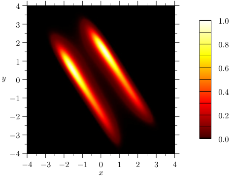
In the resulting Ulam matrix, the maximum value on the diagonal is less than . However, the computed density, plotted in Figure 15, shows two thick spurious bands, which would be more consistent with a system with a large amount of diffusion in the slow direction (cf. the invariant density in Figure 6 computed with significantly larger flow time ).
One way to avoid this is to increase the flow time so that a typical point moves in the slow direction by an amount comparable to the size of the boxes . However, we are assuming that we do not know in advance the directions of the slow and fast dynamics. To handle this, we compute unit eigenvectors using Ulam’s method for a sequence of increasing flow times, and stop when the result stabilizes. For instance, in the axis-aligned example system (5)–(6) in Section 4.3.2, the invariant density was computed for flow times and . Using the norm , we compute and . More important than the density is the second leading eigenfunction of the Koopman operator, i.e., the eigenfunction shown in Figure 4, since this function is used to define the fiber dynamics. The corresponding differences for this computed eigenfunction are and . We view this difference as small enough that we can safely use in the computation of the eigenfunctions.
Because we are using the Euler-Maruyama method with a time-step of , this value of corresponds to iterations. However, this value of is still much smaller than the average time an orbit takes to switch between the metastable states based at and . That switching happens on the order of hundreds of units of time (as shown in Figure 2).
As a further test, we also consider the computed eigenvalues. As argued in
Section 3, the leading eigenvalues of the full dynamics
correspond to decay rates associated to the slow dynamics.
Therefore, if many of the computed eigenvalues are very close to one, it
suggests that the flow time may be too short.
For in the example system, the leading ten computed eigenvalues
(as listed in Table 1) range from 1.000 to 0.6969
which is far enough from 1 to tell us that
advection in the slow direction is being captured in the Ulam matrix.
In addition to choosing the flow time, one must also set the number of sample points in (11) or (12). Because of the relatively long flow time, starting from one box the evolved points may lie in a large number of boxes , and must be chosen large enough that each is computed to a reasonable accuracy. In all our examples, we use and a 200 by 200 grid on the region . This is a much larger region than where orbits typically lie. However, we compute everything in this larger region so that when fiber dynamics are computed, the orbit will stay in the domain with very high probability.
Once a level set is computed, the same heuristics using -distance of the computed eigenfunctions and the distance of the eigenvalues from may be used to determine a reasonable number of iterations to apply for the fiber dynamics. These showed that 20 iterations for a total flow time of was sufficient for the fiber dynamics of the example system (5)–(6) in Section 4.3.2.
An eigenfunction computed using Ulam’s method will be given
as a linear combination of the indicator
functions .
As such functions are piecewise constant, the gradient will
therefore be zero anywhere it is defined.
This gradient is not useful in defining a gradient flow as used in
Step 4 of Algorithm 4.2.
Instead, when computing for use in the algorithm
we replace by the bilinear
interpolation of values it takes on the centers of each box .
Further, as solving for the gradient flow is computationally expensive,
we employ the following shortcut.
To compute the map at a point close to the fast fiber,
evaluate the gradient at , then take to be the intersection of
the fiber with the line given by .
Since in computing the fiber dynamics the function is only evaluated
at points very close to the level set, the gradient is nearly constant on the
short path from to and so the approximation is valid.
Alternatively, at least in principle, one could have used the eigenfunctions of the transfer operator instead of those of the Koopman operator . If is an invariant density for the dynamical system , then (9) with defines a transfer operator and the invariance of the measure implies that a constant function satisfies . Numerical experiments suggest that, similar to the Koopman operator, leading eigenfunctions of are nearly constant in the fast direction of a multiscale system. The problem with this approach is that one must numerically approximate the invariant measure , say by a density function, , and use this to compute eigenfunctions of . Numerically, this is equivalent to calculating the pointwise quotient where is an eigenvalue of the transfer operator defined with respect to Lebesgue measure . For systems which involve regions of low density with close to zero, this is intractable to do numerically.
7 Discussion and outlook
We have used the transfer operator and the Koopman operator to disentangle the multiple slow and fast scales and provide an effective set of slow variables which can then be efficiently numerically integrated in time. We constructed a projection onto a slow subspace using the eigenfunctions of the Koopman operator. We then devised an algorithm to estimate the drift and diffusion terms of an assumed stochastic differential equation describing the reduced slow dynamics. This constitutes a huge computational advantage as we were able to use time steps of the order of larger to propagate forward the slow variables when compared to the full multiscale system.
There are similarities of our approach with isocommittor surfaces in transition path theory (see for example [24] for a review) and with reaction coordinates for constrained molecular dynamics (see for example [38, 39, 47, 48]). Isocommittor surfaces separate metastable states and these methods aim at calculating the associated free energy in order to determine statistics such as most likely transitions and transition rates between the meta-stable states. It was, however, noted in [22] that reaction coordinates and isocommittor functions are not necessarily slow variables. In our method the slow and fast variables are first identified, and then subsequently the reduced dynamics is provided for the slow variables, whereas reaction coordinates and isocommittor surfaces are constructed to obtain statistics of transitions between predefined sets such as meta-stable states.
In the current paper, the algorithms were described and tested in a low-dimensional setting with one-dimensional slow dynamics and two time scales. As an outlook for future research, we now discuss how one might extend these techniques to more complicated situations.
Extension to systems with multi-dimensional slow subspace: In this paper, we considered multiscale examples with one-dimensional slow dynamics, so that the mapping could be approximated by a single eigenfunction of the Koopman operator. We outline now a possible extension of our computational method to the case of a higher-dimensional slow subspace. Details are planned for further research. For a system with higher-dimensional slow dynamics, it will be necessary to approximate by a product of eigenfunctions
Then, a value defines a fiber . The fiber dynamics can be defined as where and is a mapping from a neighbourhood down to the fiber itself. As explained in Section 6, for a single eigenfunction the numerical computation of was given by the intersection of with the line through tangent to . A possible way to extend this to the general setting is to define as the intersection of with the -dimensional affine subspace through spanned by the vectors for . Then, as in Section 4.3.2, one could test the validity of the fiber dynamics by comparing the distance to the distance for an ensemble of points on .
If the dimension of the slow dynamics is not known beforehand, an automated method to find the dimension would be to test products of an increasing number of eigenfunctions until a product is found for which gives a reasonable approximation of fast dynamics. Using this definition of , Algorithm 4.2 could be implemented much as before.
Algorithm 5 might also be generalized to use a product of eigenvalues. In such a case, the would be computed as the -dimensional mean of an ensemble of the form using a product and would be computed as the covariance matrix.
The main difficulty which would arise in implementing these extensions of the algorithms to high-dimensional systems is accurate and efficient numerical approximation of the transfer operator. Currently, techniques based on Ulam’s method are mainly restricted to low-dimensional systems.
Extension to systems with more than two time scales: In this paper, we considered dynamical systems with one fast and one slow time scale. We now suggest an iterative procedure using Algorithms 4.2 and 5 (or their higher-dimensional variants) which distills the dynamics on several time scales. For ease of exposition, we present this procedure for a system with three time scales (fast, moderate and slow). Applying Algorithm 4.2 to such a system produces fiber dynamics which incorporates the dynamics of both the fast and moderate time scales. The slowest time scales can be obtained by applying Algorithm 5 to . To further isolate the moderate and fast dynamics, apply Algorithms 4.2 and 5 now to the fiber dynamics in place of the full system .
Solving for the slow variables without having to integrate forward in time the fast variables: We defined the projection to the slow subspace via the eigenfunctions of the Koopman operator. This requires the integration in time of the full dynamics, including the fast variables, needed for Ulam’s method. The transfer operator and the infinitesimal generator share the same eigenfunctions and this has been exploited to find these eigenfunctions numerically for certain systems without trajectory integration [28, 45]. Thus, it may be possible to reformulate the steps in Algorithm 1 and 2 based purely on analysing the vector field itself without numerical integration, yielding a significant speed up in computation.
Acknowledgments
References
- [1] V. Arnold, V.V. Kozlov, and A.I. Neishtadt, Mathematical Aspects of Classical and Celestial Mechanics, Springer-Verlag, New York, 1993.
- [2] I. Babuška and J. E. Osborn, Finite element-Galerkin approximation of the eigenvalues and eigenvectors of selfadjoint problems, Math. Comp., 52 (1989), pp. 275–297.
- [3] V. Baladi and L.-S. Young, On the spectra of randomly perturbed expanding maps, Comm. Math. Phys., 156 (1993), pp. 355–385.
- [4] Nils Berglund and Barbara Gentz, Noise-Induced Phenomena in Slow-Fast Dynamical Systems, Springer, 2005.
- [5] Michael Blank, Gerhard Keller, and Carlangelo Liverani, Ruelle-Perron-Frobenius spectrum for Anosov maps, Nonlinearity, 15 (2002), pp. 1905–1973.
- [6] Chris Bose and Gary Froyland, Strange eigenmodes for invertible measure-preserving systems. in preparation.
- [7] Petra Boxler, A stochastic version of the centre manifold theorem, Probab. Th. Rel. Fields, 83 (1989), pp. 509–545.
- [8] John P. Boyd, Chebyshev and Fourier spectral methods, Dover Publications Inc., Mineola, NY, second ed., 2001.
- [9] J. Carr, Applications of Centre Manifold Theory, no. 35 in Applied Mathematical Sciences, Springer, 1981.
- [10] A.J. Chorin and O.H. Hald, Stochastic Tools in Mathematics and Science, STAMS, Springer-Verlag, New York, 2006.
- [11] A.J. Chorin, O.H. Hald, and R. Kupferman, Optimal prediction and the Mori-Zwanzig representation of irreversible processes, Proceedings of the National Academy of Science, 97 (2000), p. 2968Ð2973.
- [12] R. Coifman, I. Kevrekidis, S. Lafon, M. Maggioni, , and B. Nadler, Diffusion maps, reduction coordinates and low dimensional representation of stochastic systems, SIAM Multiscale Modeling and Simulation, 7 (2008), pp. 842–864.
- [13] R. Coifman and S. Lafon, Diffusion maps, Applied and Computational Harmonic Analysis, 21 (2006), pp. 5–30.
- [14] D. Crommelin and E. Vanden-Eijnden, Diffusion estimation from multiscale data by operator eigenpairs, Multiscale Modeling & Simulation, 9 (2011), pp. 1588–1623.
- [15] D. T. Crommelin and E. Vanden-Eijnden, Reconstruction of diffusions using spectral data from timeseries, Communications in Mathematical Sciences, 4 (2006), pp. 651 – 668.
- [16] Michael Dellnitz, Gary Froyland, and Stefan Sertl, A conjecture on the existence of isolated eigenvalues of the Perron-Frobenius operator, in International Conference on Differential Equations, Vol. 1, 2 (Berlin, 1999), World Sci. Publ., River Edge, NJ, 2000, pp. 1030–1032.
- [17] Michael Dellnitz and Oliver Junge, On the approximation of complicated dynamical behavior, SIAM J. Numer. Anal., 36 (1999), pp. 491–515.
- [18] M. Dellnitz and O. Junge, On the approximation of complicated dynamical behaviour, SIAM J. Numer. Anal., 36 (1999), pp. 491–515.
- [19] P. Deuflhard, W. Huisinga, A. Fischer, , and C. Schütte, Identification of almost invariant aggregates in nearly uncoupled Markov chains, SIAM J. Numer. Anal., 315 (2000), p. 3959.
- [20] P. Deuflhard and C. Schütte, Molecular conformation dynamics and computational drug design, in Applied Mathematics Entering the 21th Century, J. M. Hill and R. Moore, eds., ICIAM 2003, Sydney, 2004.
- [21] Weinan E, Analysis of the heterogeneous multiscale method for ordinary differential equations, Comm. Math. Sci., 1 (2003), pp. 423–436.
- [22] , Principles of Multiscale Modelling, Cambridge University Press, 2011.
- [23] Weinan E, Björn Engquist, X. Li, W. Ren, and Eric Vanden-Eijnden, Heterogeneous multiscale methods: A review, Comm. Comp. Phys., 2 (2007), pp. 367–450.
- [24] Weinan E and Eric Vanden-Eijnden, Metastability, conformation dynamics, and transition pathways in complex systems, in Multiscale Modelling and Simulation, Sabine Attinger and Petros Koumoutsakos, eds., vol. 39 of Lecture Notes in Computational Science and Engineering, Springer Berlin Heidelberg, 2004, pp. 35–68.
- [25] Gary Froyland, Computer-assisted bounds for the rate of decay of correlations, Comm. Math. Phys., 189 (1997), pp. 237–257.
- [26] G. Froyland, Statistically optimal almost-invariant sets, Physica D, 200 (2005), p. 205219.
- [27] Gary Froyland, On Ulam approximation of the isolated spectrum and eigenfunctions of hyperbolic maps, Discrete Contin. Dyn. Syst., 17 (2007), pp. 671–689 (electronic).
- [28] Gary Froyland, Oliver Junge, and Péter Koltai, Estimating long-term behavior of flows without trajectory integration: the infinitesimal generator approach, SIAM J. Numer. Anal., 51 (2013), pp. 223–247.
- [29] Gary Froyland and Kathrin Padberg, Almost-invariant sets and invariant manifolds—connecting probabilistic and geometric descriptions of coherent structures in flows, Phys. D, 238 (2009), pp. 1507–1523.
- [30] G. Froyland, K. Padberg, M. England, , and A.M. Treguier, Detection of coherent oceanic structures via transfer operators, Physical Review Letters, 98 (2007), p. 224503.
- [31] G. Froyland, N. Santitissadeekorn, and A. Monahan, Transport in time-dependent dynamical systems: Finite-time coherent sets, Chaos, 20 (2010), p. 043116.
- [32] C. W Gardiner, Handbook of Stochastic Methods for Physics, Chemistry, and the Natural Sciences, Springer, New York, 3rd ed., 2003.
- [33] B. Gaveau and L. S. Schulman, Multiple phases in stochastic dynamics: Geometry and probabilities., Physical Review E, 73 (2006), p. 036124.
- [34] C.W. Gear and I. Kevrekidis, Projective methods for differential equations, SIAM J. Sci. Comp., 24 (2003), pp. 1091–1106.
- [35] Dror Givon, Raz Kupferman, and Andrew Stuart, Extracting macroscopic dynamics: model problems and algorithms, Nonlinearity, 17 (2004), pp. R55–R127.
- [36] G. A. Gottwald and J. Harlim, The role of additive and multiplicative noise in filtering complex dynamical systems, Proc. Roy. Soc. A, 469 (2013), p. 20130096.
- [37] Georg A. Gottwald and Ian Melbourne, Homogenization for deterministic maps and multiplicative noise, Proceedings of the Royal Society A: Mathematical, Physical and Engineering Science, 469 (2013).
- [38] Carsten Hartmann and Christof Schütte, A geometric approach to constrained molecular dynamics and free energy, Commun. Math. Sci., 3 (2005), pp. 1–20.
- [39] Carsten Hartmann and Christof Schütte, Comment on two distinct notions of free energy, Physica D: Nonlinear Phenomena, 228 (2007), pp. 59–63.
- [40] W. Just, H. Kantz, C. Rödenbeck, and M. Helm, Stochastic modelling: replacing fast degrees of freedom by noise, J. Phys. A, 34 (2001), pp. 3199–3213.
- [41] I. Kevrekidis and G. Samaey, Equation-free multiscale computation: algorithms and applications, Ann. Rev. Phys. Chem., 60 (2009), pp. 321–344.
- [42] I. G Kevrekidis, C. W. Gear, J. M. Hyman, G. K. Panagiotis, O. Runborg, and C. Theodoropoulos, Equation-free, coarse-grained multiscale computation: Enabling microscopic simulators to perform system-level analysis, Comm. Math. Sci., 1 (2003), pp. 715–762.
- [43] R. Z. Khasminsky, On stochastic processes defined by differential equations with a small parameter, Theory of Probability and its Applications, 11 (1966), pp. 211–228.
- [44] P. E. Kloeden and E. Platen, Numerical methods for stochastic differential equations, in Nonlinear dynamics and stochastic mechanics, CRC Math. Model. Ser., CRC, Boca Raton, FL, 1995, pp. 437–461.
- [45] P. Koltai, Efficient approximation methods for the global long-term behavior of dynamical systems - Theory, algorithms and examples, PhD thesis, Technische Universität München, 2010.
- [46] T. G. Kurtz, A limit theorem for perturbed operator semigroups with applications to random evolutions, Journal of Functional Analysis, 12 (1973), pp. 55–67.
- [47] Tony Lelièvre, Free Energy Computations: A Mathematical Perspective, Imperial College Press, 2010.
- [48] Tony Lelièvre, Mathias Rousset, and Gabriel Stoltz, Langevin dynamics with constraints and computation of free energy differences, Mathematics of Computation, 81 (2012), pp. 2071–2125.
- [49] Tien Yien Li, Finite approximation for the Frobenius-Perron operator. A solution to Ulam’s conjecture, J. Approximation Theory, 17 (1976), pp. 177–186.
- [50] H. W. Lilliefors and C. C. McBride, Kolmogorov-Smirnov and Anderson-Darling statistics with parameters estimated by linear combinations of order statistics and some robustness properties, in Goodness-of-fit (Debrecen, 1984), vol. 45 of Colloq. Math. Soc. János Bolyai, North-Holland, Amsterdam, 1987, pp. 369–376.
- [51] W. Liu and G. Haller, Strange eigenmodes and decay of variance in the mixing of diffusive tracers, Physica D, 188 (2004), pp. 1–39.
- [52] J. Maclean and G. A. Gottwald, On convergence of the projective integration method for stiff ordinary differential equations, Communications in Mathematical Sciences, 12 (2014), pp. 235–255.
- [53] Andrew J. Majda, Ilya Timofeyev, and Eric Vanden Eijnden, A mathematical framework for stochastic climate models, Communications on Pure and Applied Mathematics, 54 (2001), pp. 891–974.
- [54] MATLAB, version 7.10.0 (R2010a), The MathWorks Inc., Natick, Massachusetts, 2010.
- [55] Ian Melbourne and Andrew Stuart, A note on diffusion limits of chaotic skew-product flows, Nonlinearity, 24 (2011), pp. 1361–1367.
- [56] Igor Mezić, Spectral properties of dynamical systems, model reduction and decompositions, Nonlinear Dynam., 41 (2005), pp. 309–325.
- [57] , Analysis of fluid flows via spectral properties of the Koopman operator, in Annual review of fluid mechanics. Volume 45, 2013, vol. 45 of Annu. Rev. Fluid Mech., Annual Reviews, Palo Alto, CA, 2013, pp. 357–378.
- [58] Igor Mezić and Andrzej Banaszuk, Comparison of systems with complex behavior, Phys. D, 197 (2004), pp. 101–133.
- [59] L. Mitchell and G. A. Gottwald, Data assimilation in slow-fast systems using homogenized climate models, Journal of the Atmospheric Sciences, 69 (2012), pp. 1359–1377.
- [60] H. Mori, H. Fujisaka, and H. Shigematsu, A new expansion of the master equation, Prog. Theor. Phys., 51 (1974), pp. 109–122.
- [61] N. Namachchivaya and G. Leng, Equivalence of stochastic averaging and stochastic normal forms, J. Appl. Mech., 57 (1990), pp. 1011–1017.
- [62] N. Namachchivaya and Y.K. Lin, Method of stochastic normal forms, Int. J. Non-Linear Mechanics, 26 (1991), pp. 1011–1017.
- [63] G C Papanicolaou, Some probabilistic problems and methods in singular perturbations, Rocky Mountain Journal of Mathematics, 6 (1976), pp. 653–674.
- [64] Grigoris A Pavliotis and Andrew M Stuart, Multiscale Methods: Averaging and Homogenization, Springer, New York, 2008.
- [65] Anthony J. Roberts, Normal form transforms separate slow and fast modes in stochastic dynamical systems, Physica A, 387 (2008), pp. 12–38.
- [66] J.A. Sanders and F. Verhulst, Averaging methods in nonlinear dynamical systems, vol. 59 of Applied Mathematical Sciences, Springer-Verlag, New York, 1985.
- [67] C. Schütte, W. Huisinga, and P. Deuflhard, Transfer operator approach to conformational dynamics in biomolecular systems, in Ergodic Theory, Analysis, and Efficient Simulation of Dynamical Systems, B. Fiedler, ed., Springer, Berlin, 2001, pp. 191–223.
- [68] Peter Sjögren, Operators associated with the Hermite semigroup—a survey, in Proceedings of the conference dedicated to Professor Miguel de Guzmán (El Escorial, 1996), vol. 3, 1997, pp. 813–823.
- [69] P. Stinis, Higher order Mori-Zwanzig models for the Euler equations, SIAM Multiscale Modeling and Simulation, 6 (2007), pp. 741–760.
- [70] S. M. Ulam, A collection of mathematical problems, Interscience Tracts in Pure and Applied Mathematics, no. 8, Interscience Publishers, New York-London, 1960.
- [71] J. Walter and C. Schütte, Conditional averaging for diffusive fast-slow systems: A sketch for derivation, in Analysis, Modeling and Simulation of Multiscale Problems, A. Mielke, ed., Springer, Berlin, 2006, pp. 647–682.
- [72] R. Zwanzig, Ensemble method in the theory of irreversibility, J. Chem. Phys., 33 (1960), pp. 1338–1341.
- [73] Robert Zwanzig, Nonequilibrium Statistical Mechanics, Oxford University Press, Oxford, 2001.