Evolution of autocatalytic sets in a competitive percolation model
Abstract
The evolution of autocatalytic sets (ACS) is a widespread process in biological, chemical and ecological systems which is of great significance in many applications, such as the evolution of new species or complex chemical organizations. In this paper, we propose a competitive model with a -selection rule in which an abrupt emergence of a macroscopic independent ACS is observed. By numerical simulations, we find that the maximal increase of the size grows linearly with the system size. We analytically derive the threshold where the abrupt jump happens and verify it by simulations. Moreover, our analysis explains how this giant independent ACS grows and reveals that, as the selection rule becomes more strict, the phase transition is dramatically postponed, and the number of the largest independent ACSs coexisting in the system increases accordingly. Our research work deepens the understanding of the evolution of ACS and should provide useful information for designing strategies to control the emergence of ACS in corresponding applications.
1 Introduction
Complex networks [1] are often used to describe a variety of chemical, biological and social systems. For instance, the metabolism of a cell is a network of substrates and enzymes interacting via chemical reactions [2, 3]. Ecosystems are networks of biological organisms with predator-prey, competitive or symbiotic interactions [4, 5]. In real-world systems, these networks are by no means static. On the contrary, biological or chemical networks often evolve into certain structure to optimize functionality according to some mechanisms. It is shown that the small-world structure of metabolic networks may have evolved to enable a cell to react rapidly to perturbations [2]. Similarly, the visual cortex may have evolved into a small-world architecture since it would aid the synchronization of neuron firing patterns [6]. Therefore, understanding the mechanisms responsible for the evolution of such networks is an important issue in many applications.
To explore the mechanisms underlying the network evolution, a set of models based on artificial chemistry of catalyzed reactions are proposed [7, 8, 9, 10]. An artificial chemistry is a system whose components react with each other in a way analogous to molecules participating in chemical reactions. This kinds of systems are widespread in biological research, such as the protein or enzymes within a cell [2, 3], or some organic molecules in a pool on the prebiotic Earth [11]. The networks evolve over time as mutation happens [12, 13, 14], and the structure of networks will in turn affect the subsequent evolutions. With these models, questions about self-organization, the origin of life and other evolvability issues are explored in works on artificial chemistries [7, 8, 9, 10].
Based on this framework, Bak and Sneppen [12] introduced a simple and robust model of biological evolution of an ecology of interacting species, which had the feature that the least fit species mutated. The model self-organized into a critical steady state with intermittent coevolutionary avalanches of all sizes [12]. Later on, inspired by the Bak-Sneppen model, Jain and Krishna [13, 14] proposed a similar model, in which the mutation of a species also changed its links to other species. They investigated how the network of interactions among the species evolved over a longer time scale and the growth of the autocatalytic set (ACS) [13]. It was shown that, starting from a sparse random graph, an ACS inevitably appeared and triggered a cascade of exponentially increasing connectivity until it spanned the whole graph.
The concept of an ACS is introduced in the context of a set of catalytically interacting molecules. It is defined to be a set of molecular species that contains, within itself, a catalyst for each of its member species [15, 16, 17]. Mathematically, in a graph of interacting agents, an ACS is defined as a subgraph whose every node has at least one incoming link from a node that belongs to the same subgraph [13]. This definition is meant to capture the property that an ACS has ”catalytic closure” [7], i.e., it contains the catalysts for all its members. Therefore, autocatalytic sets might be more stable to perturbations because of their ability to self-replicate. On the prebiotic Earth, autocatalytic sets are suggested as one of the possible means by which a complex chemical organization could have evolved [18]. Due to its property of self-replicating, the ACS plays an important role in the overall dynamics in chemical or biological networks. As defined, an ACS may have several disconnected components. These components are independent units that posses property of self-replicating. We define each component as an independent ACS and focus on the largest one in this paper, which contains the largest number of species.
The definition of the largest independent ACS is somewhat analogous to that of the giant component (GC) in percolation transition [19]. Percolation can be interpreted as the formation of a giant component in networks. One important model to show this process is the classic Erdós and Rényi (ER) [20] model. In ER model, the evolution proceeds as follows: Starting with isolated nodes, an edge is connected between a randomly selected unconnected pair of nodes at each time step. Then as the number of connected edges increases, a macroscopic cluster, i.e., the giant component, appears at the percolation threshold, and its size grows continuously. Recently, based on the ER model, an explosive percolation (EP) [21] model was introduced. In this model, the ER model was modified by imposing additionally a so-called product rule or sum rule, which suppresses the formation of a large cluster [21]. Because of this suppressive bias, the percolation threshold is delayed. When the giant component eventually emerges, it does so explosively. This result has attracted much interest [22, 23, 24, 25, 26, 27, 28, 29, 30, 31, 32]. Initially, this explosive phase transition was regarded as a discontinuous transition. However, it was recently found that the transition is continuous in the thermodynamic limit [28], followed by a mathematical proof [29] and extensive supporting simulations [30, 31, 32].
Inspired by the EP model, we propose an evolving network model that presents an abrupt emergence of the largest independent ACS. By imposing a selection rule [25, 26, 27], the formation of ACS’s largest component is suppressed. In the next section, we introduce the definition of this competitive model, and then discuss its properties. After that, we give an analytical analysis of the threshold where a macroscopic independent ACS appears. The theoretical results are verified by simulations. In the last section, we conclude our findings and give a brief discussion.
2 Model
The system is described by a directed graph, in which the nodes represent the species or chemicals and the directed links stand for catalytic interactions between them. The graph can be completely described by an adjacency matrix , where if there exists a link from node to , and zero otherwise. A directed link from node to means that is catalyzed by . Specifically, we exclude the self-replicating species, i.e. for all .
According to the definition, an ACS may consist of several disjoint smaller ACSs, which have no intersections with each other and form as independent catalytic systems. To describe this fact, we introduce the concept of independent ACS. Concretely, for the nodes in ACS, an independent ACS is the maximal weakly-connected subgraph which is only composed of ACS-nodes. For example, in Fig.1(a), there are three independent ACSs marked with red color. Notice that, node and do not belong to the independent ACS since they are not ACS-nodes, even though they have links connecting to independent ACSs. Denote the size of independent ACSs as in descending order. Particularly, since there may be several independent ACSs with the same size , we denote them as . Here represents the number of independent ACS with size . For convenience, we simply denote as the set of the independent ACSs with size . Based on the definition of ACS, is still an ACS with nodes. In this paper, we focus on the largest independent ACSs (), which usually play the most important role of self-replicating in the evolution process.
At the beginning time , the initial graph is a random graph with average indegree (or outdegree) (i.e. the probability of linking a directed edge is ). For every discrete time step , we denote as the number of the independent ACSs in at time . The graph is updated as follows:
Step 1. Select ”most mutating” nodes in the network. This procedure is performed based on a special set named least fitness [13], which will be explained later.
Step 2. For each of the selected nodes , determine the size of the largest independent ACS in the new network if node is updated. The update associated with node processes as follows: for node , remove all the incoming and outgoing links attached to it, and then replace them by links randomly connected to other nodes with the same probability . So for each selected node , we get a new adjacency matrix and a new largest size of the independent ACS .
Step 3. Randomly select a node with , where is the size of the largest independent ACS before the update. If all the are larger than original , we just choose one node uniformly from the selected nodes. Then the network is updated to .
At each time step, we need to select nodes with ”least fitness”. To achieve this, each node is assigned a population and a relative population , where . Between two successive graph updates, the evolution of population is given by
| (1) |
From the above equation, has the dynamics
| (2) |
In this model, we can use to measure the fitness of the species in the environment defined by the graph. The larger is, the more fit species is. So the nodes with smallest values of are picked as the ”most mutating” nodes. Moreover, when reaches to the stable solution, the value of is zero for almost all the nodes outside the ACS. Therefore, before ACS spans across the whole graph, the selected nodes are almost outside the ACS.

Fig.1 illustrates the rule of the model with . At some step, two nodes and are selected from the set least fitness and one of them will be updated. In the case of Fig.1(b), the update of node will not affect the size of the largest independent ACS. Whereas, in Fig.1(c), node will join in the largest independent ACS, making its size increase by 1. According to the rule, node will be picked as the updating node since it will not increase the size of the largest independent ACS.
When , our model degenerates to the classic ACS evolutionary model [13], in which the size of ACS grows exponentially. However, if is larger than , the evolution process will present essential difference. Specifically, the size of the largest independent ACS will ”jump” by the size of at one single step. This discontinuous increase stems from the coexistence of several independent ACSs with maximal size during the evolution. We are interest in the number of the largest independent ACSs that the system can maintain in the process. In the next section, we will discuss this phenomenon in more details.
3 Properties
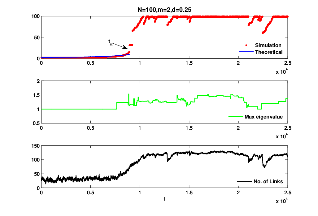
Since the evolution process of the model with has been investigated in [13], we focus on the situation where is larger than . Fig.2 shows the evolution process of the model with , and . Before the first ACS appears, almost all the nodes are in the least fitness set. Based on this fact, every graph can be roughly assumed as a sample of the classical ER directed random networks. In the evolution, usually the first ACS is generated in the form of a cycle, which is also the simplest pattern of ACS. When we update a single node, according our assumption, a cycle will appear with the probability , where is the probability of forming a cycle of size . As we select nodes at every step, according to the selection rule, the probability of forming a cycle will be . If taking as the time that the first ACS appears, the distribution of can be approximated by a geometric distribution with , and the expectation of is . Although is very large, the appearance of an ACS is inevitable. For convenience, take as the beginning time in Fig.2. Before , both and maximal eigenvalue are always zero, and the number of links fluctuates around the expectation value .
In Fig.2(a), an abrupt jump of is observed at time . This is different from the continuous growth of ACS in the classical model. We will explain this in more details later. In Fig.2(b), we present the evolution of the largest eigenvalue of . Based on the graph theory, we can get following conclusions [13]: (1) An ACS always contains a cycle. (2) If a graph has no ACS, then the largest eigenvalue is zero. (3) If a graph has an ACS, then the largest eigenvalue is larger than . There is no ACS before , so the largest eigenvalue keeps zero in this period. As shown in Fig.2(c), the number of links changes dramatically when grows to the whole graph or collapses down in Fig.2(a). Both the curves in Fig.2(a) and (c) have the same tendency, and they also have a strong relationship with the least fitness set.

The nature of the discontinuous jump of is better revealed in Fig.3. The maximal increase of the largest independent ACS is linear with the system size for . With this trend, we have . This evidence from simulation shows that our model can lead to an abrupt emergence of a macroscopic independent ACS. In the evolution process, there are several large independent ACSs coexisting and finally merging together to overtake the previous largest one. With the increase of , it is more difficult for to grow. As the suppression strengthens, the system can maintain more largest independent ACSs, and there will be less nodes outside the ACS. Moreover, it is almost impossible to break up a large ACS into smaller ones since the updating nodes mostly don’t belongs to ACSs. For large , the increase of will mainly depend on merging two giant independent ACSs rather than adding isolated nodes. In the next section, we will analyze this process theoretically and perform simulations to verify the results.
4 Theoretical analysis
Based on the investigation above, it is clear that the models with and are very different. In [13, 18], the properties of the model with have been discussed with analytical method, so in this section we will analyze the model with . First, we consider the probability of adding a node to the ACS that has nodes (donated as ). Based on the definition of ACS, a node could be added to ACS if and only if there is an incoming link from the ACS to this node. So the probability is:
| (3) |
Here is the probability of linking an edge in update. As our model is applied to sparse graphs, in which the linking probability is very small, Eq.3 can be approximated by
| (4) |
At each time step, we only update one node out of the selected nodes. The size would change if all the nodes had at least one incoming link from . The size of is and based on Eq.4, we can calculate the average change of for the sparse graph
| (5) |
If we take the first time that an independent ACS appears as the beginning step , Eq.5 can be integrated from to
| (6) |
Taking as the initial size of , the equation above can be written as follows
| (7) |
For the last part of the Eq.7, we define a quantity such that . In fact, can be viewed as the average tolerance of the largest independent ACSs during the evolution. In other words, the larger is, the more largest independent ACSs the system can maintain. With this definition, we get the function of for different values of
| (8) |
The evolution function for should be , which presents an exponential and continuous increase of the ACS size. This is quite different from the function of above. For the parameter , when takes certain value, the denominator in Eq.8 will become zero. Therefore, we identify a phase transition at some time step . The threshold is
| (9) |
or
| (10) |


Fig.4 and Fig.5 are the numerical results with and respectively. Because of the assumption of the sparse graph, we choose the average indegree from to . For fixed value of , we perform the simulations starting from an initial ACS with size on random graphs. To determine the threshold, in simulations we take the time step where the increase of the largest independent ACS’s size exceeds of the system size as . Since the starting time is set to , we rearrange Eq.10 as follows
| (11) |
Therefore, there is a linear relation between the quantity and . In Fig.4 and Fig.5, there is clearly a linear relation between these two quantities, and the numerical results agree with the fitting line very well. To check the fitting errors for different system sizes, we define the fitting error as the average distance from the data points to corresponding fitting line. For both cases, the fitting errors decrease as the system size increases.
Moreover, from the slope (donated as ) of the fitting line we can obtain by relation
| (12) |
In order to compare with the real number of the largest independent ACSs coexisting in the system during the evolution, we record this number in each time step in simulations. Then we take the average of these values as the real . Table.1 and Table.2 display the results of from both the theoretical analysis and simulations. As increases from to , grows a lot, which means more strict suppression will make the system maintain more largest independent ACSs during the evolution process. This fact will further lead to the result that the jump of enhances a lot when increases, as shown in Fig.3. Besides, as the system size grows, also increases slightly. This is a natural result of the increase of system size. Therefore, the choice of will dramatically affect the formation of the giant independent ACS, both the emergence time and the jump of size.
| 2.7092 | 3.2034 | 3.4603 | 3.6747 | 3.9670 | |
| 2.7234 | 3.1138 | 3.4057 | 3.6424 | 3.8506 | |
| 0.52% | 2.88% | 1.60% | 0.89% | 3.02% | |
| 2.6455 | 2.9722 | 3.3169 | 3.5234 | 3.7140 | |
| 2.4982 | 2.8377 | 3.1036 | 3.3963 | 3.5553 | |
| 5.90% | 4.74% | 6.87% | 3.74% | 4.46% | |
| 2.4724 | 2.6988 | 3.0940 | 3.2862 | 3.5529 | |
| 2.2683 | 2.5943 | 2.8485 | 3.0770 | 3.3001 | |
| 8.99% | 4.03% | 8.62% | 6.80% | 7.66% |
| 7.3929 | 9.1257 | 10.8941 | 11.7463 | 12.9772 | |
| 7.2431 | 8.7351 | 10.3443 | 11.3490 | 12.4997 | |
| 2.07% | 4.47% | 5.31% | 3.50% | 3.82% | |
| 6.4972 | 7.9128 | 9.2004 | 10.3262 | 11.1204 | |
| 6.1639 | 7.4202 | 8.6414 | 9.8103 | 10.5035 | |
| 5.41% | 6.64% | 6.47% | 5.26% | 5.87% | |
| 5.5494 | 6.9597 | 8.1509 | 9.0114 | 9.9579 | |
| 5.2646 | 6.4332 | 7.4965 | 8.3728 | 9.2047 | |
| 5.41% | 8.18% | 8.73% | 7.63% | 8.18% |
5 Conclusions
ACS is an important concept in the evolution dynamics of biological, chemical and ecological systems. The emergence of an ACS is often used to explain the mechanism by which a complex chemical organization or species could have evolved. In this paper, by imposing a -selection rule, we propose a competitive model to investigate the evolution process of ACS under suppression. In this model, we observe a discontinuous phase transition where a microscopic independent ACS appears abruptly. The increase of its size is found to grow linearly with the system size by simulations. We derive the threshold analytically and verify our result through numerical simulations on different system sizes and various choices of . As the suppression increases, the phase transition is dramatically deferred. Furthermore, we explore the evolution process of the largest independent ACS. To quantify the tolerance of the system to the emergence of a microscopic independent ACS, we define a quantity that describes the average number of largest independent ACSs during the evolution process. It is shown increases as the selection rule becomes more strict. Therefore, on average, a system with larger would contain more largest independent ACSs during the evolution. Our model gives a possible explanation for the sudden appearance of a class of species or chemical organizations in specific situations. By only introducing a selection rule, the evolution of ACS presents qualitative difference with that of the classical model. Our study sheds light on the research of evolutional process of ACS and provides helpful instructions to design effective strategies to control the appearance of ACS in practice.
6 Acknowledgements
This work is supported by the National Natural Science Foundation of China No. 11290141 and No. 11201019.
References
- [1] R. Albert and A.-L. Barabási, Statistical mechanics of complex networks, Rev. Mod. Phys. 74, 47-97 (2002).
- [2] D.A. Fell and A. Wagner, The small-world of metabolism, Nature Biotechnology 18, 1121-1122 (2000).
- [3] H. Jeong, B. Tombor, A. Albert, Z.N. Oltvai, and A.-L. Barabási, The large-scale organization of metabolic networks, Nature 407, 651-654 (2000).
- [4] R.J. Williams and N.D. Martinez,Simple rules yield complex food webs, Nature 404, 180-183 (2000).
- [5] J. Camacho, R. Guimerà, and L.A.N. Amaral, Robust patterns in food web structure, Phys. Rev. Lett. 88, 228102 (2002).
- [6] D.J. Watts and S.H. Strogatz, Collective dynamics of ’small-world’ networks, Nature 393, 440-442 (1998).
- [7] S.A. Kauffman, Autocatalytic sets of proteins, J. Theor. Biol. 119, 1-24 (1986).
- [8] J.D. Farmer, S.A. Kauffman, and N.H. Packard, Autocatalytic replication of polymers, Physica D: Nonlinear Phenomena 22, 50-67 (1986).
- [9] W. Fontana and L.W. Buss, ”The arrival of the fittest”: Toward a theory of biological organization, Bull. Math. Biol. 56, 1-64 (1994).
- [10] P.F.Stadler, W. Fontana, and J.H. Miller, Random catalytic reaction networks, Physica D: Nonlinear Phenomena 63, 378-392 (1993).
- [11] G.F. Joyce, RNA evolution and the origins of life, Nature 338, 217-223 (1989).
- [12] P. Bak and K. Sneppen, Punctuated equilibrium and criticality in a simple model of evolution, Phys. Rev. Lett. 71, 4083-4086 (1993).
- [13] S. Jain and S. Krishna, Autocatalytic Sets and the Growth of Complexity in an Evolutionary Model, Phys. Rev. Lett. 81, 5684-5687 (1998).
- [14] S. Jain and S. Krishna, Crashes, recoveries, and ¡°core shifts¡± in a model of evolving networks, Phys. Rev. E 65, 026103 (2002).
- [15] M. Eigen, Selforganization of matter and the evolution of biological macromolecules, Naturwissenschaften 58, 465-523 (1971).
- [16] S.A. Kauffman, Celluar homeostasis, epigenesis and replication in randomly aggregated macromolecular systems, J. Cybernetics 1, 71-96 (1971).
- [17] O.E. Rossler, A system theoretic model of biogenesis, Z. Naturforschung 26b, 741-746 (1971).
- [18] S. Jain and S. Krishna, A model for the emergence of cooperation, interdependence and structure in evolving networks, Proc. Natl. Acad. Sci. U.S.A. 98, 543-547 (2001).
- [19] D. Stauffer and A. Aharony, Introduction to Percolation Theory (Taylor & Francis, London, ed. 2, 1994).
- [20] P. Erdös and A. Rényi, On the evolution of random graphs, Publ. Math. Inst. Hungar. Acad. Sci 5, 17 (1960).
- [21] D. Achlioptas, R.M. D’Souza, and J. Spencer, Explosive Percolation in Random Networks, Science 323, 1453 (2009).
- [22] R.M. Ziff, Explosive Growth in Biased Dynamic Percolation on Two-Dimensional Regular Lattice Networks, Phys. Rev. Lett. 103, 045701 (2009).
- [23] F. Radicchi and S. Fortunato, Explosive Percolation in Scale-Free Networks, Phys. Rev. Lett. 103, 168701 (2009).
- [24] N.A.M. Araújo and H.J. Herrmann, Explosive Percolation via Control of the Largest Cluster, Phys. Rev. Lett. 105, 035701 (2010).
- [25] Y.S. Cho, S. Hwang, H.J. Herrmann, and B. Kahng, Avoiding a Spanning Cluster in Percolation Models, Science 339, 1185-1187 (2013)
- [26] W. Chen and R.M. D’Souza, Explosive Percolation with Multiple Giant Components, Phys. Rev. Lett. 106, 115701 (2011).
- [27] R. Zhang, W. Wei, B. Guo, Y. Zhang, and Z. Zheng, Analysis on the evolution process of BFW-like model with discontinuous percolation of multiple giant components, Physica A 392, 1232-1245 (2013)
- [28] R.A. da Costa, S.N. Dorogovtsev, A.V. Goltsev, and J.F.F. Mendes, Explosive Percolation Transition is Actually Continuous, Phys. Rev. Lett. 105, 255701 (2010).
- [29] O. Riordan and L. Warnke, Explosive Percolation Is Continuous, Science 333, 322-324 (2011).
- [30] P. Grassberger, C. Christensen, G. Bizhani, S. Son, and M. Paczuski,Explosive Percolation is Continuous, but with Unusual Finite Size Behavior, Phys. Rev. Lett. 106, 255701 (2011).
- [31] H.K. Lee, B.J. Kim, and H. Park, Continuity of the explosive percolation transition, Phys. Rev. E 84, 020101(R) (2011).
- [32] N. Bastas, K. Kosmidis, and P. Argyrakis, Explosive site percolation and finite-size hysteresis, Phys. Rev. E 84, 066112 (2011).
- [33] B. Bollobas, Random Graphs, 2nd ed., Academic Press, New York, (2011).