Single-molecule-mediated heat current between an electronic and a bosonic bath

The most direct realization of the model given by Eq. (1) is that of a single molecule adsorbed on a metallic surface. Adsorbed molecules on surfaces have been intensely studied over the years, both theoretically and experimentally (for a brief review see Ref. [23]).

In such molecules, the vibrational modes of adsorbed molecules relax by interaction with the surface conductance electrons as well as by coupling to the bulk phonons, and the interaction between the electrons and the vibrational mode plays an important role. [13] One of the common models used to describe such interactions [24] is the Hamiltonian of Eq. (1), prior to the reduction of the relevant conductance electrons degrees of freedom to one-dimensional fields. Adopting that description, the bosonic bath described by the operators $\gamma_{n}$ and $\gamma^{\dagger}_{n}$ in our Hamiltonian represent the bulk phonons. The molecule is then brought into contact with an STM-tip or other electronic lead, and the conductance electrons couple to the electronic level on the molecule. Focusing on the electronic mode that couples to the molecule, we can map them onto the one-dimensional field that is represented by the electronic field operators $\psi(x)$ and $\psi^{\dagger}(x)$ in the Hamiltonian. A detail of the process can be found in Ref. [25]. In such a system, generally one would take $\epsilon_{d}=0$, as the conductions electrons are held in resonance with the electronic level on the molecule.

Another system that can be described by the model of Eq. (1) is that of a molecular bridge — a single molecule sandwiched between two electronic leads. In such single-molecule devices the electron-phonon interaction plays an important role, as the molecular orbitals are coupled simultaneously to the lead electrons and to the vibrational modes of the molecule itself. The molecular bridge is typically placed on an insulating substrate which provides an additional phononic bath that couples to the molecular vibrational modes. [26, 27]

Focusing on a molecular junction held between leads with no bias voltage, one can choose a symmetric and anti-symmetric basis for the lead electrons, thus the molecule interacts with an effective single electronic band. The molecule itself is modeled by a single spinless electronic level $d^{\dagger}$ with energy $\epsilon_{d}$ which is coupled by displacement to a local vibrational mode $b^{\dagger}$ with frequency $\Omega_{0}$. This vibrational mode is further coupled by displacement to a bath of phonons $\gamma^{\dagger}_{n}$. The level is then coupled to the single band of electrons via a hopping matrix element $t$. The resulting Hamiltonian is given by

with $\hat{n}_{d}=d^{\dagger}d$ and

Typically the Hamiltonian is treated either in the weak-coupling limit using perturbation theory in $g$, or using the Lang-Firsov transformation [28] and the polaronic approximation in the limit where $t$ is small. In the limit of a broad level close to resonance, however, this Hamiltonian can be reduced [25, 29] to the continuum limit Hamiltonian of Eq. (1) as described in detail in Ref. [25]. This mapping process give rise to an effective high-energy cutoff which is determined by the hybridization width of the level $\Gamma=\pi\rho_{0}t^{2}$. The effective bandwidth $D_{\rm eff}$ of the continuous field $\psi(x)$ is related to the hybridization width by $D_{\rm eff}=\pi\Gamma/2$.

The final system considered is an Aharonov-Bohm interferometer with a molecular device embedded in one of its arms. This setup is a more complicated variant of the molecular bridge described above, as there is an additional transmission channel between the two leads, and a magnetic flux $\varphi$ threading the ring. Lately, this system has attracted a considerable interest, following the work of Entin-Wohlman and others [6, 7] who computed the transport coefficients relating the linear-response electric and heat currents to the voltage bias and temperature gradient.

Restricting our attention to the case where the two electronic leads are held in identical temperature and chemical potential, the Hamiltonian describing such a device is given [32] by $\mathcal{H}=\mathcal{H}_{0}+\mathcal{H}_{L,R}+\mathcal{H}_{\rm dot}$, with

Here, $\mathcal{H}_{0}$ describes the left (L) and right (R) lead electrons, $\mathcal{H}_{L,R}$ describes the arm of the interferometer without the device, and $\mathcal{H}_{\rm dot}$ describes the device itself and its coupling to the leads. The general term $\mathcal{H}_{\rm int}$ may contain any local interactions at the dot that do not involve the lead electrons. In our case, it will include the local vibrational mode, the electron-phonon coupling and the bosonic bath. However, for the purpose of the mapping shown here, no further assumptions are needed on the form of $\mathcal{H}_{\rm int}$ beyond it not involving the lead electrons.

We begin by transferring to the symmetric and anti-symmetric basis, defining the new symmetric field

where $\psi_{L/R}(x)=\sum_{k}e^{i\epsilon_{k}x/v_{F}}c_{k,L/R}$. The Green function $G_{\psi\psi^{\dagger}}(z)$ pertaining to this field at $x=0$ can now be calculated from the Green functions of the left and right fields at the origin, given by matrix form as

Using this we write the dot’s Green function as

where $\Sigma_{\rm int}(z)$ is the self-energy contribution of the $\mathcal{H}_{\rm int}$. Close to resonance, the role of the symmetric electronic Green function $G_{\psi\psi^{\dagger}}$ will be to renormalize $\epsilon_{d}$ and the level width. Therefore, our effective Hamiltonian of eq. (1) generates the same correlation functions pertaining to the dot operators as the original Hamiltonian, ensuring the validity of the calculations of the heat current. To this end, we have to adjust the parameters of our effective Hamiltonian such that the effective electronic band-width is

with $\bar{\Gamma}=(\Gamma_{L}+\Gamma_{R})/(1+x)$, where

The renormalized level energy is effected by the flux threading the ring

where $\alpha=4\Gamma_{L}\Gamma_{R}/(\Gamma_{L}+\Gamma_{R})^{2}$.

As the flux $\varphi$ contributes only to the effective $\epsilon_{d}$, which will be shown to effect the heat current only at quartic orders or through the renormalization of the coupling coefficient $g$, one concludes that the magnetic flux effects the heat current similarly. Moreover, its effect is an even function of the flux.

To compute the heat current we begin by writing it in the form

where

In steady state all two-time correlation functions reduce to a function of the time difference only. This allows one to convert to the energy domain by Fourier transforming with respect to the time difference. We apply this procedure to $G^{>}_{b,n}(t,t^{\prime})$, and aiming at evaluating

we resort to ordinary diagrammatic perturbation expansion to write an expression for $G_{b,n}^{>}(\epsilon)$. To this end, it is useful to define the free (i.e., $\lambda_{n}=0$) Green functions of the bath bosons in matrix form as

for the retarded and advanced functions, and

for the lesser and greater functions, where $n_{b}(\epsilon)=1/(e^{\beta_{b}\epsilon}-1)$ is the Bose-Einstein distribution function corresponding to the temperature $T_{b}$. Similarly, we shall denote the fully dressed Green functions of the molecular vibrational mode $b^{\dagger}$ by $G^{r,a}(\epsilon)$ and $G^{<,>}(\epsilon)$, for which the $2\!\times\!2$ matrix notation

is used. [The same $2\!\times\!2$ matrix notation applies to $g^{\nu}_{\gamma,n}(\epsilon)$ above.]

Having laid out the building blocks for the perturbation expansion, we rely on Langreth theorem [35] to have the identity, at steady-state

which we shall now turn to evaluate.

Focusing initially on the retarded and advanced Green functions $G^{r,a}(\epsilon)$, these acquire the form

where

are the corresponding self-energy functions. There are two contributions to $\Sigma^{r,a}(\epsilon)$: one due to the coupling to the electronic bath [the first term on the right-hand side of Eq. (35)], and another due to the coupling to the bosonic bath [the second term on the right-hand side of Eq. (35)]. Denoting these two terms by $\Sigma^{r,a}_{\,e}(\epsilon)$ and $\Sigma^{r,a}_{\,b}(\epsilon)$, respectively, the former can be expressed in a closed analytical form [25] in terms of the Exponential Integral function: [36]

Here, $\rho_{0}=1/(2\pi v_{F})=1/(2aD_{\rm eff})$ is the density of states per unit length, and $\xi$ equals $\epsilon/D_{\rm eff}$. As for the second contribution $\Sigma^{r,a}_{\,b}(\epsilon)$, it can be conveniently expressed in terms of the coupling function $\Lambda(\omega)$,

For an Ohmic bath with $s=1$, Eq. (37) can be evaluated in closed analytic form to obtain

Proceeding to the lesser and greater Green functions $G^{<,>}(\epsilon)$, these read

with the lesser and greater self-energy functions

Here, $n_{e}(\epsilon)=1/(e^{\beta_{e}\epsilon}-1)$ is the Bose-Einstein distribution function corresponding to the temperature $T_{e}$. Note that Eq. (40) can be conveniently related to the two components of the retarded self-energy through

which generalizes the standard equilibrium relation $\Sigma^{<,>}(\epsilon)=\mp 2n(\pm\epsilon){\rm Im}\{\Sigma^{r}_{e}(\epsilon)\}$.

To evaluate $G^{>}_{b,n}(t,t)$ of Eq. (33), it is useful to utilize the identities

which follow directly from Eqs. (34) and (39). Here we have introduced the auxiliary function

and made use of the fact that $\Sigma^{a}(\epsilon)=\left[\Sigma^{r}(\epsilon)\right]^{\ast}$. Inserting these identities into Eq. (33) one obtains

which reduces by virtue of Eq. (41) to

Plugging this result into Eq. (27), employing the relations $g(-\epsilon)=g^{\ast}(\epsilon)$ and $[n_{e}(-\epsilon)-n_{b}(-\epsilon)]=-[n_{e}(\epsilon)-n_{b}(\epsilon)]$, and exploiting the fact that $\Lambda(\epsilon)$ is restricted to positive energies, we finally arrive at

where we have explicitly written out the function $|g(\epsilon)|^{2}$ that appears in the integrand [see Eq. (43)].

Equation (46) is the central result of this paper. It provides an exact expression for the heat current corresponding to the bosonic Hamiltonian of Eq. (21), for a general coupling function $\Lambda(\epsilon)$. Since $[n_{e}(\epsilon)-n_{b}(\epsilon)]$ with $\epsilon>0$ is positive definite for $T_{e}>T_{b}$ (negative definite for $T_{b}>T_{e}$), the heat current flows, as it physically should, from the hotter bath to the colder one. Below we analyze in detail the characteristics of $J_{Q}$ in different temperature and coupling regimes.

The form of expression for the heat current bears a similarity to Landauer formula. Other works studying thermal conductance through local contacts have arrived at a similar expressions or used a Landauer-type expression as a starting point. [9, 8, 2, 10] In the context of heat current between bosonic reservoirs this expression was derived in earlier works discussing Hamiltonians similar to the one in eq. (21) [15, 18, 16]. This type of expression survives even when accounting perturbatively for the interaction with vibrational modes. [5]

We begin with the low-temperature limit, $T_{e},T_{b}\ll\Omega_{0}$ (throughout this paper we assume that $\Omega_{0}<\omega_{c},D_{\rm eff}$). In this limit, the Bose-Einstein distribution functions $n_{e}(\epsilon)$ and $n_{b}(\epsilon)$ that enter the integrand of Eq. (46) have decayed long before $e^{-\epsilon/D_{\rm eff}}$ and $|g(\epsilon)|^{2}$ have changed in any significant manner from their $\epsilon=0$ values. Thus, to a good approximation one can (i) set $e^{-\epsilon/D_{\rm eff}}|g(\epsilon)|^{2}\to|g(0)|^{2}$ in the integrand of Eq. (46), and (ii) extend the upper integration limit to infinity. Taking the coupling function $\Lambda(\epsilon)$ to have the power-law form of Eq. (3) this yields

The resulting integral can now be carried out analytically using

where $\zeta(x)$ is the Riemann zeta function. [37] This in turn gives

with $A=(4\pi\rho_{0}\tilde{g}\Omega_{0})^{2}\alpha\omega_{c}^{1-s}|g(0)|^{2}\Gamma(3+s)\zeta(3+s)$. Lastly, $g(0)$ has the explicit expression

allowing one to express the coefficient $A$ entirely in terms of the basic model parameters entering the bosonic Hamiltonian of Eq. (21).

As can be seen from Eq. (49), the low-temperature heat current shows a rather strong temperature dependence. In particular, the linear-response heat conductance

varies as $T^{2+s}$, corresponding to $T^{3}$ for an Ohmic bath. This should be contrasted with the heat conductance of a generic noninteracting electronic tunnel junction, which varies linearly with $T$ at sufficiently low temperature. [38] For the heat conductance of a tunnel junction to display a superlinear temperature dependence of the form found here, its transmission coefficient must vanish in a power-law fashion at the Fermi energy.

This power-law behavior of the heat current at low temperatures was also observed for systems in which the two bosonic reservoirs are connected by a system with few degrees of freedom such as in the spin-boson model [17, 19]. The similarity between these systems and the system under consideration here, at low-temperatures with respect to $\Omega_{0}$, stems from the fact that at this temperature regime only the lowest lying levels of the vibrational mode of the molecule are available for transferring energy between the baths.

As commented above, an Ohmic bath with $s=1$ is of particular interest. Focusing on this case and on the hierarchy $\Omega_{0},T_{e},T_{b}\ll\min\{D_{\rm eff},\omega_{c}\}$, we devise below an analytical expression for the nonequilibrium heat current, encompassing the crossover from the low-temperature regime, $\max\{T_{e},T_{b}\}\ll\Omega_{0}$, to the intermediate-temperature one, $\Omega_{0}<\max\{T_{e},T_{b}\}$. This expression is approximate as it employs a power series expansion of the self-energies, but yields accurate results within the regime where $D_{\rm eff}$ and $\omega_{c}$ are the largest energy scales in the system.

To this end, consider the function $g(\epsilon)$ which enters the integrand of Eq. (46). Since the Bose-Einstein distribution functions $n_{e}(\epsilon)$ and $n_{b}(\epsilon)$ decay on a scale far smaller than $\min\{D_{\rm eff},\omega_{c}\}$, it suffices to accurately represent $g(\epsilon)$ for $\epsilon\ll\min\{D_{\rm eff},\omega_{c}\}$. This allows one to expand the exact expressions for $\Sigma^{r}_{e}(\epsilon)$ and $\Sigma^{r}_{b}(\epsilon)$ [see Eqs. (36) and (38) above] in $x=\epsilon/D_{\rm eff}$ and $y=\epsilon/\omega_{c}$ to obtain

Settling with linear orders in $x$ and $y$, the function $g(\epsilon)$ is well approximated for $\epsilon\ll\min\{D_{\rm eff},\omega_{c}\}$ by

where $z_{\pm}$ equals $\pm\tilde{\Omega}-i/\tau$ with the softened frequency

and the relaxation rate

The softened frequency $\tilde{\Omega}$ characterizes the dressed excitations of the phonon, and thus serves as the energy scale which determines the cross over from the high-temperature to the low-temperature behavior. Within this approximation for $g(\epsilon)$, the heat current for an Ohmic bath becomes

where we have set in addition $e^{-\epsilon/D_{\rm eff}}\to 1$ and extended the upper integration limit to infinity (both approximations being well justified by the hierarchy $T_{e},T_{b}\ll\min\{D_{\rm eff},\omega_{c}\}$). The resulting integral in Eq. (57) can be performed in a closed analytic form in terms of the digamma function [39] $\psi(z)$. Skipping details of the algebra we quote here only the end result:

It is straightforward to confirm using the asymptotic expansion [39]

that Eq. (58) properly reduces for $T_{e},T_{b}\ll\tilde{\Omega}$ to Eq. (49) with $s=1$, including the precise value of the prefactor $A$. More interesting is the limit $\tilde{\Omega}<\max\{T_{e},T_{b}\}$, when the leading contribution to Eq. (58) crosses over to a linear dependence on the temperature difference $\Delta T=(T_{e}-T_{b})$. Thus, as the larger of the two temperatures exceeds the vibrational resonance energy, the heat current continues to increase linearly with $\Delta T$. This behavior markedly differs from that of a resonant electronic tunnel junction, whose heat current depends logarithmically on $\Delta T$ above the resonance energy. The physical difference stems, as we show below, from the bosonic nature of the vibrational mode, which can be excited to exceedingly high energies by creating ever more phonons. This should be contrasted with a resonant electronic level, which can only be empty or occupied.

Having analyzed analytically certain limits, we now proceed to a complete numerical evaluation of the exact heat current of Eq. (46) at arbitrary temperatures $T_{e}$ and $T_{b}$. As the temperatures $T_{e}$ and $T_{b}$ enter the expression for the heat current only through the term $[n_{e}(\epsilon)-n_{b}(\epsilon)]$ in the integrand, it is anti-symmetric under replacing them. As such, we may restrict ourselves to calculations in which $T_{b}$ is held constant and the heat current is calculated for different values of $T_{e}$, and generalize the results for opposite values by inverting the direction of the current.

In Fig. 2 we have addressed the case where one bath (the bosonic one) is held at a constant low temperature $T_{b}/\Omega_{0}=10^{-4}$, while scanning different values of $T_{e}$ higher than that temperature. We have plotted the heat current in the case of a sub-Ohmic bath (with $s=1/2$), an Ohmic bath and a super-Ohmic bath (with $s=1$). The graph shows a clear crossover from a power-law behavior to a linear dependence as $\Delta T$ increases to values of the order of $\Omega_{0}$. In the inset of the graph we have plotted, on a log-log scale, the heat current for small values of $\Delta T$ for each type of bath, and a dashed line following the expected power-law behaviors at low temperatures given at Eq. (49). The agreement between the calculated heat current and the expected one is excellent while $T_{e}\ll\Omega_{0}$, breaking at about $T_{e}/\Omega_{0}\simeq 0.1$. Figure 3 describes the heat current as well, but focuses on the case where the temperature of the bosonic bath is held at the high value of $T_{b}=\Omega_{0}$. In this case the heat current about $\Delta T=0$ displays a linear dependence on $\Delta T$, with different slope for every type of bosonic bath.

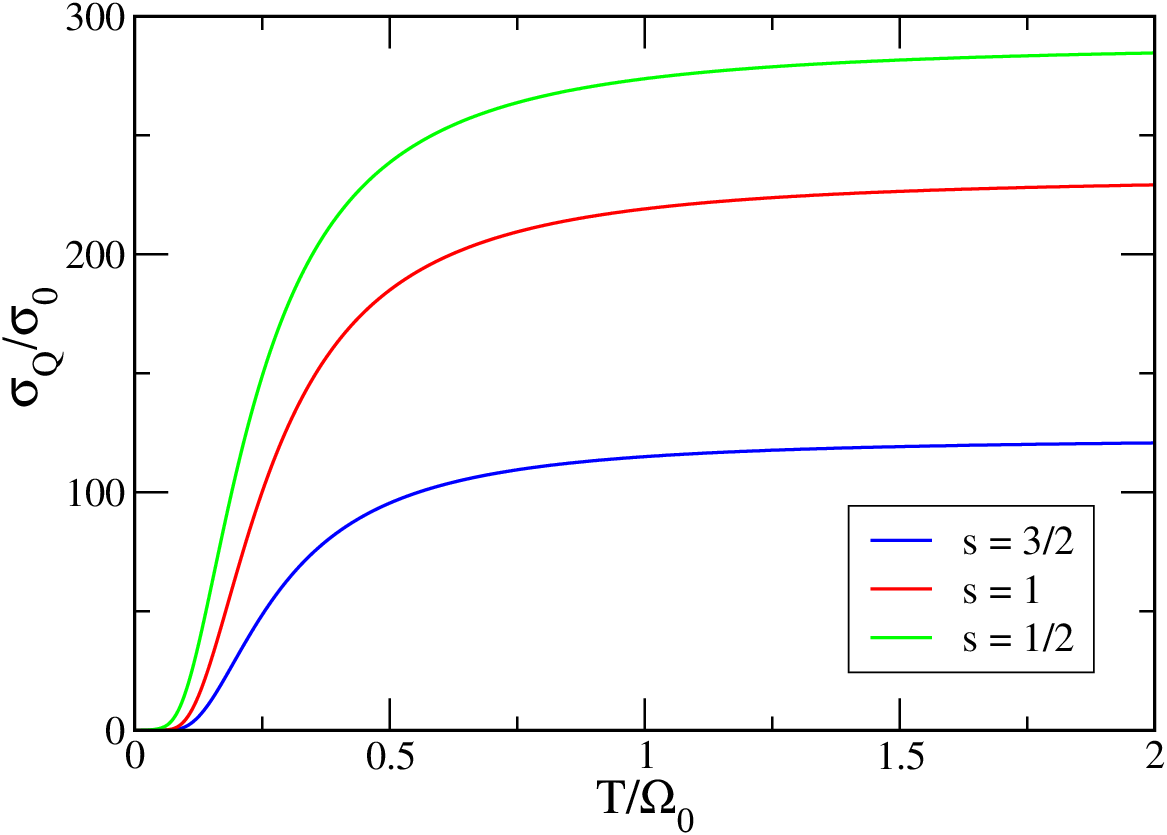
In Fig. 4 we have plotted the linear-response heat conductance $\sigma_{Q}$, as defined in Eq. (51), for different temperatures and types of baths. As the temperatures rises, the conductance increases until it saturates at about $T\simeq\Omega_{0}$. The different exponents relating to the type of bosonic baths are evident in the low-temperature regime.

It is useful to define at this point the reduced transition rates