An Improved Bayesian Semiparametric Model for Palaeoclimate Reconstruction: Cross-validation Based Model Assessment
Abstract
Fossil-based palaeoclimate reconstruction is an important area of ecological science that has gained momentum in the backdrop of the global climate change debate. The hierarchical Bayesian paradigm provides an interesting platform for studying such important scientific issue. However, our cross-validation based assessment of the existing Bayesian hierarchical models with respect to two modern proxy data sets based on chironomid and pollen, respectively, revealed that the models are inadequate for the data sets.
In this paper, we model the species assemblages (compositional data) by the zero-inflated multinomial distribution,
while modelling the species response functions using Dirichlet process based Gaussian mixtures. This modelling strategy
yielded significantly improved performances, and a formal Bayesian test of model adequacy, developed recently, showed
that our new model is adequate for both the modern data sets. Furthermore, combining together the zero-inflated assumption,
Importance Resampling Markov Chain Monte Carlo (IRMCMC) and the recently developed Transformation-based Markov Chain
Monte Carlo (TMCMC), we develop a powerful and efficient computational methodology.
Keywords: Cross-validation; Dirichlet Process; Palaeoclimate Reconstruction; Response Function;
Transformation Based Markov Chain Monte Carlo; Zero-inflated Multinomial.
1 Introduction
The science of palaeoclimate reconstruction involves predicting prehistoric climate changes by studying fossil records of species abundances (assemblages) preserved in lake sediments and a ‘modern, training data set’ consisting of known records of species abundances and climate values at different sites in the ‘modern time’, where modern time is conventionally defined as the time period from the year 1950 till present. Broadly, methods of palaeoclimate reconstruction consist of two steps. The first step is to calibrate a relationship between the observed species abundances and the observed climates using the modern, training data. It is generally assumed that the species abundances depend upon climate, not the other way. In this sense, the calibration step is a ‘forward’ problem. Then, assuming that the calibrated relationship holds good even in the past ages where fossil records of the species are available but not the prehistoric climates, the calibrated relationship is ‘inverted’ to obtain reconstructions of the past climates. Thus, the problem of climate reconstruction is an inverse problem.
In the current scenario of the climate change discussion, the problem of palaeoclimate reconstruction has gained much importance. In this context, the Bayesian model-based attempt of the Irish climate reconstruction using pollen assemblages by ? (henceforth, HWB), is a particularly welcome contribution. The model builds upon the palaeoclimate model of ? (henceforth, VTK) who considered the multinomial Dirichlet model for the compositional data of chironomid assemblages (non-biting midges, well-known for providing accurate information regarding past climates; see ?), and used the unimodal Gaussian function to describe the responses of the different species to climate. By unimodal Gaussian response function we mean that the expectation of the number of any particular species is a bell-shaped function of climate; there is an optimum climate value at which the species is expected to thrive the most, and deviation from the optimum climate leads to an exponential decrease in the expected number of the species.
The main modeling contribution of HWB is to propose a nonparametric approach to modelling the species response function. The reason for considering a new approach to modeling the response surfaces is that the unimodal Gaussian response function is too simplistic and may not be adequate for most of the species since the species are expected to respond differently to environmental changes, indicating that the response functions may vary from species to species, apart from being complex in nature. For a detailed discussion regarding these issues, see ?.
But in spite of the commendable attempt and the sensible results related to Irish climate reconstruction, some issues related to the model of HWB should not be overlooked. Firstly, their nonparametric model for the response surface, which is based on lattice Gaussian Markov Random Field (GMRF) (see, for example, ?), introduces a lot of parameters (around 10,000) which makes computation burdensome. Secondly, for higher dimensional climate variables the climate grid may not be feasible to construct; moreover, this would involve too many parameters, rendering computation infeasible as well. Thirdly, the unknown past climate variables are assumed to take values in the region formed by the modern climate values, which need not be an appropriate assumption for general palaeoclimate problems.
In an effort to rectify these problems, ? (henceforth, SB) modeled the response functions as a mixture of unknown number of Gaussian functions, while using the multinomial Dirichlet distribution to model the compositional data. He applied this model to the modern training data set consisting of (modern) chironomid counts obtained from 62 lakes of Finland along with the corresponding modern temperatures, also analysed by VTK. The results of leave-one-out cross-validation showed that in 83% cases the true temperature values are included in the 95% credible intervals associated with the posteriors of SB. This was a significant improvement over the model of VTK, which had just 43% coverage of the true temperature values.
However, before applying any potential palaeoclimate model to climate reconstruction, it is desirable to validate it as rigorously as possible. Indeed, with respect to the chironomid data neither the model of VTK nor that of SB satisfy the model adequacy test developed in ? (see also ?). It is shown in ? that the model of HWB, involving the pollen data, also fails the model adequacy test, even though coverage of the observed climate values GDD5 (growing degree days above C) and MTCO (mean temperature of the coldest month) have been quite satisfactory. As demonstrated in ? (Chapter 7), the model of HWB overfits the pollen data. In fact, although the predicted climates (modes of the posterior distributions) and the observed climates agree well with each other, the posterior distributions have large credible regions, indicating high uncertainty. Such large credible regions are responsible for the poor fit (overfit). Presumably, many of the parameters related to the response surfaces were not adequately informed by the data. Indeed, as can be seen from Figure 5 of HWB, many of the small lattice squares of the climate grid hardly contain any data point. Due to the Markov property of the GMRF assumption the parameters associated with such lattice squares do not depend upon distant lattice squares containing enough data; hence, these parameters do not have information from the data to reduce their posterior variabilities. Hence, the credible regions turned out to be too large, resulting in overfit.
In this paper, we shall conern ourselves with assessment of model adequacy via cross-validation of the training data. We shall not attempt actual climate reconstruction in this paper. In particular, we present a hierarchical zero-inflated multinomial model for the compositional fossil data and, following SB, propose a mixture of unknown number of Gaussian functions to model the response function of each species. The only difference between this model and that of SB is the zero-inflated multinomial model in place of the ordinary mutinomial model. But importantly, this apparently simple modification resulted in quite significant improvement of the results previously obtained by SB. Indeed, with our zero-inflated multinomial model and mixtures of unknown number of Gaussian functions, in the case of the chironomid data of VTK we have been able to include approximately 97% of the observed temperature values in our respective 95% highest posterior density (HPD) credible regions, 3 cases only marginally missing the HPD regions. More encouragingly, our model satisfies the model adequacy test proposed in ?. Generalising our ideas to the pollen data case of HWB we show that our model satisfies the test of adequacy even for the pollen data – the cross-validation exercise associated with the pollen data showed inclusion of approximately 95% observed climate values in the respective 95% HPD regions. Indeed, in the aforementioned previous works on palaeoclimate reconstruction, the count data, characterized by a large number of zeroes (about 59% zeroes in the chironomid case and about 37% zeroes in the case of pollen), rendered the ordinary multinomial distribution inappropriate.
Apart from the very much improved results, our model and methods facilitate very fast and efficient computation, which is crucial for palaeoclimate reconstruction where the data sets tend to be (at least moderately) large. For the cross-validation purpose we combine the Importance Resampling Markov Chain Monte Carlo (IRMCMC) methodology of ? with the recently developed Transformation based Markov Chain Monte Carlo (TMCMC) (?) to further improve computational efficiency. A brief overview of TMCMC is provided in Section 3.1; here we just note that TMCMC allows updating high-dimensional parameter vectors using simple deterministic transformations of one-dimensional random variables having arbitrary distributions on some relevant support.
It is worth mentioning that recently ? have developed a nested Dirichlet-Multinomial model for multivariate pollen counts data. Their work is motivated by ?; however, their need to use the integrated nested Laplace approximation (INLA) (?) for the purpose of fast computation, also played a very significant role in their model-building procedure. In particular, ? specify a model which exploits the nested structure within the pollen species based on botanic similarities; within each level of the nested structure the species proportions are assumed to be Beta/Dirichlet, and conditionally independent of the other levels consisting of the other species, given their GMRF prior on the two-dimensional climate grid (same as that of HWB, and so this model also precludes extrapolation and is difficult to generalize for high-dimensional climate variables) and other hyperparameters. At each level, the count data is then assumed to be zero-inflated Binomial/Multinomial, given the proportions at that level of the nested structure. The conditional independencies, although undesirable, are necessary for INLA implementation. Thus, although INLA has greatly sped up their computation, the method did demand sacrifice of model flexibility. Also, although INLA has been appropriate for the cross-validation summary statistics that ? consider, it is perhaps the case that INLA, being a deterministic approach, can not approximate the posterior distrbutions of arbitrary discrepancy measures, for example, those that we consider in this paper; see also ? for a brief discussion.
The rest of our paper is structured as follows. In Section 2 we propose our new model for the chironomid data. Fitting our model using MCMC is discussed in detail in Section 3, and our method of leave-one-out cross-validation using IRMCMC is provided in Section 4. Cross-validation of the chironomid data and detailed analysis of the results of the cross-validation are presented in Section 5. The formal model adequacy test, along with its application to the chironomid data using posterior samples from the cross-validation exercise, are discussed in Section 6. In Section 7 we generalize our model and methods to the pollen data of HWB, while cross-validation of the pollen data and subsequently the model adequacy test are discussed in Sections 8 and 9, respectively. We finally conclude with some discussion on future work in Section 10. Additional details are provided in the supplement ?, whose sections and figures have the prefix “S-” when referred to in this paper.
2 An improved model for the chironomid data
Before proceeding we briefly review the data set, the full description of which can be found in ?; see also VTK.
2.1 Brief description of the data set
As already mentioned in the introduction, chironomids are non-biting midges, and considered very suitable for past climate reconstruction. The modern, training data set analysed by VTK consists of counts of chironomid head capsules present in the top 1 cm surface-sediment from 62 lakes located mainly in northwestern Finnish Lapland. Recorded also are site-specific mean July air temperatures, estimated for each lake using 1961–1990 Climate Normals data from 11 nearby climate stations (2 in Norway, 5 in Finland, and 4 in Sweden) and applying consistent regional lapse rates and linear interpolation (see ? for details). After excluding rare species, 52 taxa of chironomid were finally selected.
Thus, the chironomid data of VTK consists of modern time assemblages for species of chironomid, along with the mean July temperature values at each of lakes (sites) in Finland. This modern, training data set has been used by ? for reconstructing past climates of Finland using VTK’s model.
In the following subsections of this present section we provide details of semiparametrically modelling this data. The same model will be generalised to the case of the pollen data of HWB in Section 7. In what follows, we begin with the zero-inflated Poisson model for the count data, finally deriving from it the zero-inflated multinomial model.
2.2 Hierarchical model specification starting with zero-inflated Poisson model
For and , let denote the count of the -th chironomid species available at the -th site; let denote the complete count data set. Also, let denote the temperature at site . Let denote the complete set of temperature values. With these we consider the following mixture model for :
| (1) |
where , , denotes point mass at zero, and denotes the Poisson distribution with parameter . Further,
| (2) | ||||
| (3) |
In (2) denotes the Gamma distribution with mean and variance , where is a fixed constant. Here and are shape and scale parameters, respectively. In (3) and stand for the -th optimum temperature (-th optimum of the -th species) and the -th tolerance level (a measure of temperature within the vicinity of the optimum temperature that the species can withstand); is the maximum number of optima and the tolerance levels of the -th species. These will be further elucidated in Section 2.4.
2.3 Viewing species optima and tolerance levels as samples from Dirichlet processes
Writing , we assume that for each , is a sample from the Dirichlet process (see, for example, ?):
| (4) | ||||
| (5) |
In (5), denotes the Dirichlet process with representing the strength of the belief in the central distribution . Here we assume that under , the joint distribution of is normal-inverse-gamma, given by
| (6) |
The values of the parameters , and will be specified in the context of the application.
2.4 Response function
Introducing the allocation variables (these can also be thought of as auxiliary or latent variables) helps ascertain whether the corresponding count is zero or arose randomly from . Formally, with probability and 0 with probability . Observe that
| (7) |
showing that the response function of the -th species at the -th site is given by (7). Now, since the Dirichlet process is discrete with probability one, it follows that with positive probability, the parameters are equal. A consequence of this is the reduction of (7) to the following:
| (8) |
where, with , the set is the set of distinct values among , and is the frequency of the occurrence of . Of course, . Since the number of, and the frequencies of coincidences among the parameters is random, it is clear that (8) is a mixture of Gaussian functions with unknown number of components. Moreover, it is also clear that all the species have different response functions, with different number of mixture components. This is important, since different taxa may require different numbers of components to adequately model the response surface.
An alternative to our mixture representation of the response surfaces are spline based models for the same. For this modeling style, for different species, the orders of the splines (orders of the polynomial parts), the numbers and locations of the knots, must be treated as unknown and different. Although the part of the spline associated with the knots can be modeled using Dirichlet process, the same is not appropriate for modeling the polynomial part of the spline. The reason is that Dirichlet process can only force the polynomial coefficients to be equal with positive probability, but coincidences among the polynomial coefficients can not decrease the order of the polynomial. As such, the polynomial part must be handled using complicated variable-dimensional MCMC methods, for example, reversible jump MCMC (RJMCMC). Since complicated RJMCMC has to be carried out for all the species, this would very significantly increase the computational burden. But such computational difficulties can be overcome by a new, general, MCMC methodology for variable dimensional models, which is being developed by ?. The methdogology, which we refer to as Transdimensional TMCMC (TTMCMC) is an extension of TMCMC for variable dimensional cases, and can update all the (random number of) parameters in a single block, using deterministic transformations of some arbitrary one-dimensional random variable. This would greatly assist in computation associated with spline-based response functions that we hope to pursue in the future.
2.5 From zero-inflated Poisson to zero-inflated multinomial
Letting , it follows that the joint distribution of
is zero-inflated multinomial, given by:
| (9) |
Now note that denotes the unknown proportion of the -th species at the -th site, whenever , that is, whenever . These proportions are clearly dependent since all of them are scaled by the same sum . In fact, since a priori , it follows that . In other words, even though the species parameters are considered independent at the Poisson level, the species proportions are dependent at the multinomial level for each . Thus, we have the following Multinomial-Dirichlet structure: for ,
Although it is possible to express our Bayesian model in terms of the Dirichlet parameters and then analytically integrate out the latter, so that no longer needs to be simulated by MCMC methods, there are two reasons to retain . Firstly, are the Poisson parameters associated with the first stage of our modeling, which does not condition on ; hence it may be of interest to learn . Here note that the model in terms of (even if are retained), is not identifiable with respect to , since multiplying with some constant yields the same . Hence, if are of interest, the model must be expressed in terms of , not .
Secondly, and more importantly, retaining these parameters expand the parameter space, which may allow free movement of the MCMC sampler, thereby facilitating improved mixing. One such instance is reported in ?, where the MCMC sampler associated with the marginalized model failed to discover a minor mode of a bimodal cross-validation posterior associated with VTK’s model, but the expanded model of VTK with the Dirichlet parameters allowed the MCMC sampler to explore the mode adequately. Since multimodality plays very important roles in both of our examples, we resort to modeling in terms of . Since we update the parameters in a single step using TMCMC, retaining these parameters does not cause computational burden.
We have pointed out that although the species parameters are independent at the Poisson level, dependence is induced at the multinomial stage, via conditioning on . However, it is possible to induce dependence between the species parameters even at the Poisson level, by considering the hierarchical Dirichlet process (?). In other words, we could assume that, for , ; ; , where and is a specified distribution. The implication of such a hierarchical structure is that the parameters associated with the species response functions will be shared with positive probability by the various species, inducing dependence. However, in our set-up this would create severe computational difficulties. Again, such computation difficulties can perhaps be overcome by TTMCMC of ?. We intend to explore the issues related to the new modelling ideas and computational methods in the future.
2.6 Joint posterior
Now, letting , , , , the posterior of is given by
| (10) |
where is given by the following Polya urn scheme (?):
| (11) | ||||
| (12) |
In the expression for the joint posterior (10), we assumed that , for each . A few remarks regarding this prior choice is in order.
It is natural to choose a subjective prior on the zero-inflation probabilities which depends upon climate. However, the zero-inflation probabilities directly affect the number of zeroes in the data, and so any subjective prior, which may depend upon the climate must be chosen with great care because mis-specification in this case can easily give rise to a conflict between the data and the prior. An instance of mis-specification may be that at several locations several taxa may be completely outside its range boundary which gives rise to excess zeroes, even though the climate on which the prior of for such locations and species depend, may be optimal for those taxa. In this case the prior would not indicate excess zeroes, even though the observed data may contain excess zeroes, suggesting a conflict between the prior and the data. The objective prior cuts down such risk, as is evident from Figure 3 and 9, which indicate that the observed values are fitted well by our model and the associated priors. Moreover, the prior also serves to simplify the computations to a large extent, since the associated Gibbs step involves a simple simulation exercise from the relevant Beta distributions. It is worth mentioning that could be easily integrated out analytically from the joint posterior (10) to simplify the model, but since we are interested in the posterior of and since retaining these parameters may induce better mixing of our MCMC sampler, we did not marginalize the joint posterior with respect to .
3 Model fitting using Markov chain Monte Carlo (MCMC)
For MCMC purposes the full conditionals of the unknowns and are available in standard forms for sampling using simple Gibbs steps. It will also be observed that the full conditionals do not involve the complete likelihood thanks to the zero-inflated multinomial distribution, involving only those terms which are associated with strictly positive count data points. Since a large number of counts are zero, this provides the very important advantage of very fast and efficient computation. Updating using the Polya urn distribution as the proposal for Metropolis-Hastings steps as in SB turned out to to be quite effective here. Finally, we update in a single block using TMCMC to further enhance computational efficiency. Before proceeding further we first provide a brief overview of TMCMC.
3.1 Overview of TMCMC
TMCMC enables updating an entire block of parameters using deterministic bijective transformations of some arbitrary low-dimensional random variable. Thus very high-dimensional parameter spaces can be explored using simple transformations of very low-dimensional random variables. In fact, transformations of some one-dimensional random variable always suffices, which we shall adopt in our examples. Quite clearly, the underlying idea also greatly improves computational speed and acceptance rate compared to block Metropolis-Hastings methods. Interestingly, the TMCMC acceptance ratio is indepenent of the proposal distribution chosen for the arbitrary low-dimensional random variable. For implementation in our cases, we shall consider the additive transformation, since it is shown in ? that many fewer number of “move types” are required by this transformation compared to non-additive transformations.
To elaborate the additive TMCMC mechanism, assume that a block of parameters is to be updated simultaneously using additive TMCMC, where is some positive integer. At the -th iteration we shall then simulate , where is some arbitrary distribution and is the indicator function of the set . In our examples we shall choose to be density, so that is simulated from a truncated normal distribution. We then propose, for , with equal probability (although equal probability is a convenience, not a necessity), where are appropriate scaling constants. Thus, using additive transformations of a single, one-dimensional , we update the entire block at once. In our examples, we select the tuning parameters using information from several pilot runs of our TMCMC algorithm. In other words, we run our TMCMC algorithm several times for iterations, each time with a set of possible trial values of ; in fact, we begin with all the trial values set equal to 0.5, and then observing the mixing properties of the associated pilot run, we modify the trial values accordingly. We continue this for several pilot runs until the mixing is reasonable. We ascertain mixing informally using trace and autocorrelation plots of the sample path of the TMCMC.
The aforementioned procedure of selecting the tuning parameters, although yielded reasonable mixing, is evidently somewhat ad-hoc. A more rigorous method for choosing the tuning parameters in additive TMCMC can be based on the recenly developed optimal scaling theory for additive TMCMC by ?. Since ? show that the optimal acceptance rate for additive TMCMC under various set-ups is 0.439, one can tune the scaling constants to achieve about 44% acceptance rate. Note that for random walk Metropolis, the corresponding optimal acceptance rate is 0.234, much lower than that of additive TMCMC. Comparisons between additive TMCMC and random walk Metropolis in terms of optimal scaling are thoroughly explored in ?.
In Section S-1 of the supplement we descibe an MCMC algorithm, which is a combination of Gibbs steps, Metropolis-Hastings and TMCMC steps, for updating the unknowns. The updating procedure will be used to cross-validate our model, which we discuss below.
4 Leave-one-out cross-validation
In order to assess the validity of our model we successively leave out data point (that is, we leave out both and the assemblage ) from the training data set, and using the remaining data set along with , the latter regarded as the test data, attempt to predict . So, we must now include a new parameter, which we denote by , corresponding to the left out climate value . Now, this new parameter requires a prior. We set a prior for this new parameter.
As a referee suggests, one could also look upon as the true measurement of the climate value at the -th site, where is the observed value of the climate subject to a measurement error at site . From this perspective, the prior on can be interpreted as the prior on the true measurement of the climate variable at site . We write , where denotes the measurement error. The modified likelihood associated with this perspective is the original likelihood conditional on the observed climate values, multiplied with this normal likelihood contributed by the measurement error at the -th site. The prior for must then be duly multiplied with the joint likelihood and the priors for the other parameters to arrive at the form of the joint posterior. The observed climate coincides with the true climate if and only if , that is, when there is no measurement error. In that case, the posterior of coincides with our cross-validation posterior when is held out. Indeed, we are not aware of any evidence to suggest that there is significant climate measurement error in either the chironomid data or the pollen data. Hence, for both the applications we shall assume that the observed climate values are the true climate values, and the prior on the new parameter corresponding to the held out climate value makes sense from this perspective.
4.1 Full conditional of
The full conditional of given the rest is given by
| (13) |
where in , must be replaced with . For updating the one-dimensional variable , random walk Metropolis with appoximately optimized scaling constant will be used. In fact, ? show that a TMCMC step for updating one-dimensional parameter coincides with a Metropolis-Hasting step; in this case, the additive TMCMC step is equivalent to a random walk Metropolis step. All the other variables will be updated in the way described in Section S-1.
Now observe that since we need to perform an MCMC run for each left out data point, many computationally burdensome MCMC implementations are necessary, thus calling for innovative computational shortcuts. The usual importance sampling based ideas (see, for example, ?, ?) do not work in inverse problem set-ups such as in our case. In an inverse problem the response variable (say, ) is modeled conditional on some covariates (say, ), but prediction of some future given and the training data set , is of interest. This is a much more complicated problem compared to the usual forward situation, where prediction of is of interest, given the training data set and . Details are provided in ?. To meet the challenges of cross-validation in inverse problems, ? (see also ?) proposed a very fast and efficient methodology by judiciously combining importance re-sampling (IR) and MCMC. Here we adopt their methodology, which has been termed IRMCMC by the above authors. Details, for our current problem, are provided in Section S-2 of the supplement.
5 Cross-validation of chironomid data
For our application we fixed , , , , , , for all . These choices are motivated by VTK and SB who attempted to incorporate ecological knowledge into their priors; in particular, the choice implies that a priori the probability of a multimodal response function for the -th species is , which is slightly higher than the probability of a unimodal response function. It is also worth mentioning that using fixed value of in the context of Dirichlet process is commonplace; see, for example, ?, ?, ?, ?, ?, ?, ?, ?, ?, ?, ?.
Some remarks regarding the choice of and in general palaeoclimate problems is in order. In the paradigm of regular mixtures, that is, when the data arise from some mixture model with unknown number of components, ?, ?, ? consider Dirichlet process based mixture models of the form (3) (see also ? for Dirichlet process based mixtures in the context of circular data, and ? in the case of genetics), where upper bounds on the number of mixture components were required. For normal mixtures based on Dirichlet process, a detailed asymptotic investigation regarding asymptotic choice of the upper bound has been carried out by ?; it turned out, under suitable regularity conditions, that the form of (the upper bound allowed to increase with the sample size ) satisfying as , is adequate. Thus, for fixed sample size , one may choose to be less than . Although our current set-up is very different from regular mixture problems, as a rule of thumb, we can select to be less than , the number of sites. The asymptotic choices of ( allowed to depend upon ), again increasing with but a rate slower than that of , are shown by ? to be adequate.
For details regarding the other prior choices, see VTK and SB. We choose to allow a reasonably wide range of possible values of to be considered. As we report in Section 5.1, our cross-validation results are remarkably robust with respect to other choices of and .
For the purpose of IRMCMC we first selected as . Since is even, there are two choices of the median. Following ? we chose . For this importance sampling density, we simulated a sample of size after discarding a burn-in period of length . From these stored MCMC realizations we re-sampled, without replacement, realizations for each of the 62 cases. For each case, given each of the 200 re-sampled realizations, we then simulated, using MCMC, samples from , thus obtaining IRMCMC realizations from each of the 62 posteriors associated with leave-one-out cross-validation. The entire cross-validation exercise using IRMCMC took just about an hour. For computing the 95% HPD regions of the cross-validation posteriors , we implemented the well-known line-pushing method; see, for example, ?.
5.1 Results of cross-validation
In 96.67% of 62 cases, the observed temperature values fell within their respective 95% HPD regions, suggesting very substantial improvement of our model over those of VTK and SB. The reason for such high percentage of inclusion of the observed temperature values in the respective HPD’s is due to taking into account large number of zero counts of the data by using zero-inflated multinomial model and also due to using an appropriate species-temperature response function. The percentage of coverage remained almost unchanged for different choices of and , suggesting remarkable robustness of our cross-validation results with respect to these prior choices.
Some of the cross-validation posteriors, along with the corresponding observed , and the 95% HPD regions, are shown in Figure 1. Many of the cross-validation posteriors are multimodal, which are consequences of multiple climate preferences of the different species.
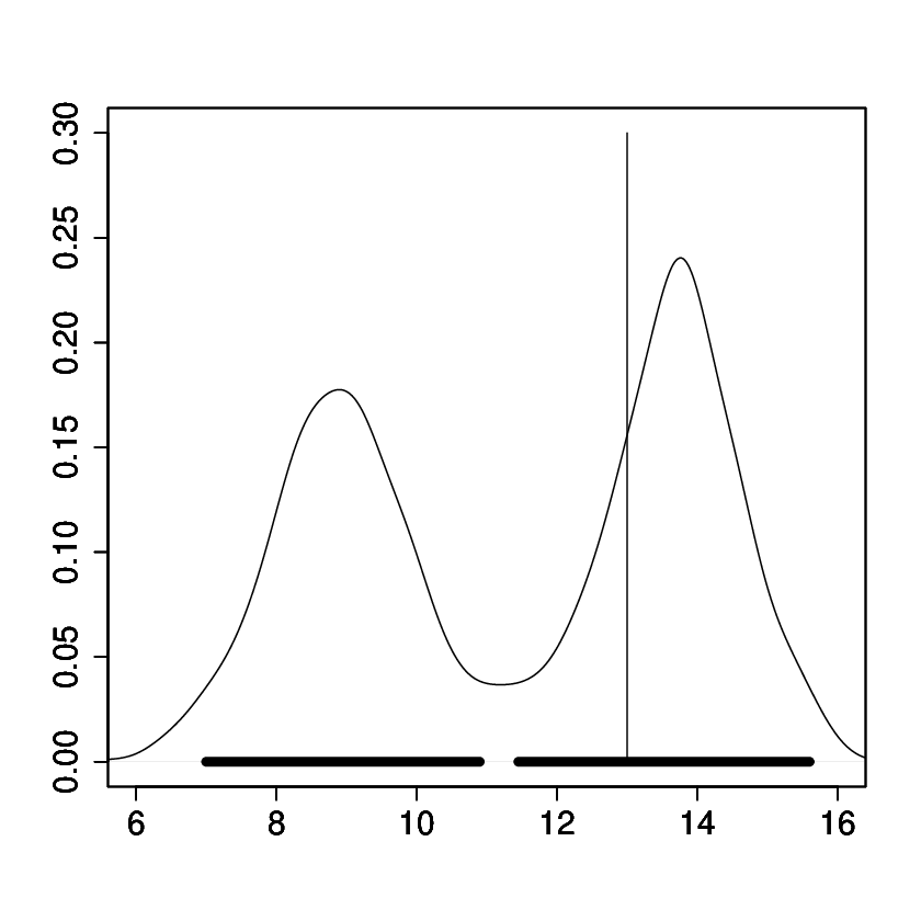
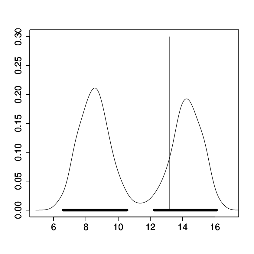
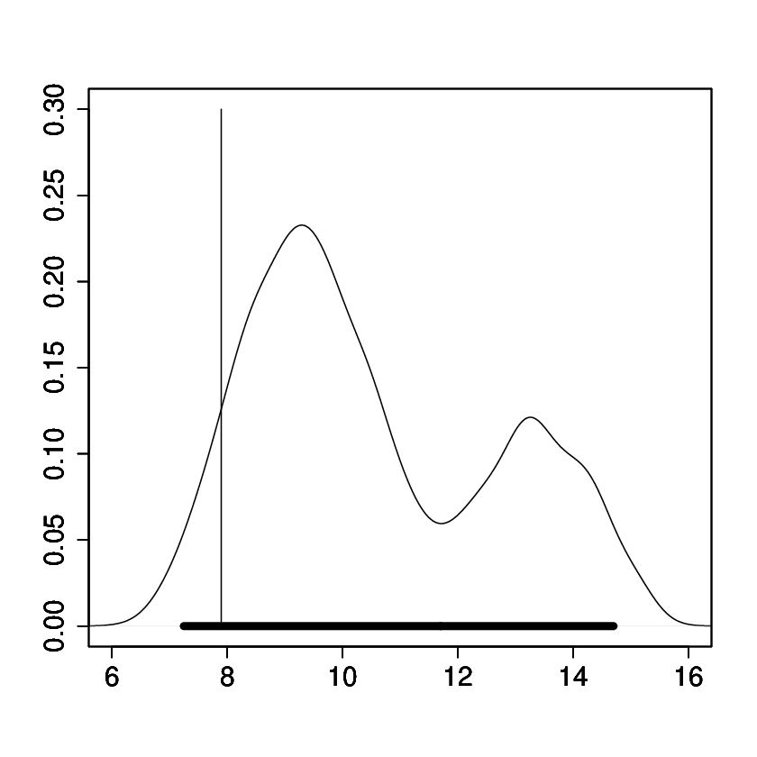
Figure 2 shows the posteriors of some of the , the probabilities of zero counts, associated with our model, under different choices of and . The displayed figures correspond to the full MCMC run for the joint posterior associated with . Considerable robustness of the posteriors of with respect to different choices of and is exhibited by the plots. Importantly, it is clearly seen that the posteriors of have modes closer to 1 than to 0 indicating that it is indeed really important to model the count data with zero-inflated multinomial distribution to account for such large proportion of zeros.


5.2 Goodness of fit of the response functions
Apart from the cross-validation results, it is also of interest to ascertain how well our Dirichlet process based response functions perform. Since this is directly related to the question of predicting the species abundances, here we consider predicting the observed species abundances using the posterior expectations of conditional on , where is the random variable associated with (or, a replicate of) the observed data point .
It follows by conditional independence, that
| (14) |
where
if . On the other hand, if , then
Thus, the posterior distribution can be studied by drawing samples from , given available MCMC samples drawn from .
We construct the predicted version of the count data for the -th species using the posterior distributions of . Figure 3 shows the respective 95% credible intervals of , joined by lines; the circles denote the count data. It is clear from the figures that a reasonably good fit is provided by our response function model.


The results of cross-validation and the fit of the response functions to the observed data may seem to be satisfactory, but a test of overall model adequacy is necessary to formally certify our new model. In the next section we address the issue of model adequacy test.
6 A test for overall model adequacy
To quote ?, assessing the plausibility of a posited model (or of assumptions in general) is always fundamental, especially in Bayesian data analysis. ? seem to be the first to attempt an extension of the essence of the classical approach of model assesment to the Bayesian framework. Their approach is based on computing the posterior distribution of the parameters given the data and then to compute a -value, involving a discrepancy measure, which is a function of the data as well as the parameters. Their approach differs from the available classical approaches mainly in introducing a discrepancy measure that depends on the parameters as well. ? introduced two alternative -values and demonstrated that they are advantageous compared to the -value of ?.
Motivated by the palaeoclimate reconstruction problem in “modern data” on fossil pollen assemblages, ? proposed a novel approach to model assesment based on “inverse reference distributions” (IRD). He has shown that his approach is suitable for assessing Bayesian model fit in inverse problems but may be extended to quite general Bayesian framework and has some distinct advantages compared to the other approaches. Here we will use the idea of ? for assessing the plausibility of our model.
The idea of ? is based on the philosophy that the model fits the data if the posterior distribution of the random variables corresponding to the non-random covariates capture the observed values of the covariates. Otherwise, the model does not fit the data. It is worth noting that although the values of the covariates are known, the model is to be fitted assuming that the values are unknown and the random variables that stand for the unknown covariates are to be predicted. The covariates predicted in this manner can then be compared with the originally observed values to assess model fit in a fully Bayesian manner.
The key idea can be mathematically formulated in the following way. Suppose represent the data and represent the non-random covariates. Let stand for the random vector associated with ; the former may also be thought of as a replicate of but must be predicted conditionally on in an inverse sense. If the posterior distribution of is consistent with observed then the model is said to have fit the data adequately. Otherwise the model is considered inadequate for the data. The fully Bayesian approach to this prediction requires computation of an inverse reference distribution based on the posterior
where denotes the likelihood of the unknowns , being the set of model parameters. ? discuss in details the advantages of using this reference distrbution. He also shows how the reference distribution may turn out to be improper and demonstrated how the leave-one-out cross-validation idea may overcome the problem of impropriety. To assess consistency of the simulated covariates with the observed values ? suggests appropriate discrepancy measures – a reference distribution of the random discrepancy measure is to be constructed using the simulated covariates ; then if , the observed discrepancy measure corresponding to the observed covariates , falls within the appropriate credible region of , the model is to be accepted, otherwise it should be rejected. The decision theoretic justification of the procedure is provided in ?.
Before applying the model adequacy test of ? we need to choose an appropriate discrepancy measure . Figure 1 shows that posterior distributions of some of the are skewed, while some are strongly indicative of multimodality. Considering the global mode of the posterior distribution of as a convenient measure of central tendency, we use the following observed discrepancy measure:
| (15) |
Replacing with in (15) yields the inverse reference distribution corresponding to . Figures 4(a), 4(b), 4(c) and 4(d) show the inverse reference distributions based on the IRMCMC simulations and the associated observed discrepancy measures corresponding to our model with (, ), (, ), (, ) and (, ), respectively. The thick, black horizontal lines represent the 95% HPD regions of the posteriors of . The vertical lines represent the observed discrepancy measures . In all the cases fall comfortably within the 95% HPD regions of the corresponding inverse reference distributions, clearly leading to acceptance of our model. We also considered several variants of the discrepancy measure (15) by replacing the mode with the median, taking sum of squares instead of sum of absolute deviations, etc. However, all these variants led to acceptance of our model.
Since the cross-validation posterior distributions of are multimodal, it is possible to question our choice of the discrepancy measure that makes use of the absolute deviation. One plausible discrepancy measure in this case may be that associated with the logarithms of the cross-validation posteriors. In other words, we may choose the following discrepancy measure:
| (16) |
Figures 5(a), 5(b), 5(c) and 5(d) display the IRMCMC-based inverse reference distributions associated with corresponding to our model with (, ), (, ), (, ) and (, ), respectively. As with , even with , the observed discrepancy measure falls comfortably within the 95% HPD region for all the four different choices of .


In Section S-3 of the supplement we investigate the relationship of the discrepancy measure with other discrepancy measures that are variants of above.
7 Generalization of our model and methods to the modern pollen data
The training data set of HWB consists of modern pollen counts on = 14 species from = 7815 different sites of the world, which we denote as before by , for . It is important to mention that unlike in the case of the chironomid data, here most of the total counts are missing. It is however known that the total counts in this case are typically . Following HWB we also treat the total counts as , that is, we take , for .
The data also includes modern, bivariate climate variables, namely, MTCO and GDD5 at those sites, which we denote as . Here we standardize and so that their sample means and variances are 0 and 1, respectively. As in the case of the chironomid data we model the pollen counts as zero-inflated multinomial of the same form as (9). Also, as in (3), is assumed to follow , where is now modelled as
| (17) |
where represents the bivariate normal density at with mean and covariance matrix . The -th element of is denoted as , . We assume that
| (18) | ||||
| (19) |
Under , is assumed to follow bivariate normal with mean vector and covariance matrix , where is a known vector. For our application we choose , matching the sample mean of the standardized climate variables GDD5 and MTCO. The reason that we select these prior parameters in this way is that the species optima , which are exchangeable, and the climate variables at which the species data are collected, are expected to be similar, and hence uncertainties about them are not expected to be very different. In fact, VTK and SB also assume the same prior mean for optimum temperature and the temperature variable.
For the prior on we assume that for , , the inverse-gamma prior with mean and variance , for . Here we choose and for so that both the prior means are 1, matching the sample (standardized) variances of and , while the prior variance is 1.3. Again, the rationale for matching the sample variances is that the species optima and the climate variables at which the species data are obtained are expected to have similar distributions. The prior variances of and are made slightly larger than the sample climate variances since the former are unobserved unlike the latter, thus incurring relatively more uncertainty. Denoting by , we put the prior on .
For this pollen data example, we choose and . Unlike the chironomid example, here setting larger values of led to overfitting the pollen data by increasing the number of mixture components in the response function (17). This suggests that the response surface in the pollen data example is expected to have less number of modes than in the chironomid data case. It is useful to remark that the choice is so common (see, for example, ?, ?, ?, ?, ?, ?, ?, etc.) that it is usually considered as the default choice in the literaure on Dirichlet process.
For the cross-validation purpose we need to select a prior for , where corresponds to the left out observed climate variable . Based on the observed sample, we set a bivariate normal prior for with means and variances for the co-ordinates of . Somewhat larger variances are chosen to account for extra uncertainty in , which is now treated as unobserved. Based on the observed sample, the covariance is taken as 0.8.
The joint posterior distribution and the forms of the full conditional distributions of the parameters can be easily calculated as in Section 2.6 and Section S-1.
8 Cross-validation of the pollen data
8.1 Implementation issues
Application of IRMCMC in the pollen data problem is carried out by first selecting = 5353 according the criterion presented in Section 4.2 of ?. We used additive TMCMC to update , , and in blocks. In fact, we apply TMCMC to the reparameterized versions of the elements of , that is, using additive TMCMC we update jointly . The reparameterized versions, being supported on the entire real line, ensures free movement of our additive TMCMC sampler, resulting in good mixing properties. It is important to mention that updating using the Polya urn distribution as the proposal distribution failed to yield satisfactory mixing. We overcame the problem by adding a TMCMC step to update the distinct components of in a single block, after Metropolis-Hastings with the Polya urn proposal has been applied sequentially to . A further step of TMCMC consisting of only two move-types with equal probabilities, either adding a single to all the variables or subtracting it from all of them with equal probabilities, using the TMCMC-based acceptance ratio to decide on the final acceptance, very significantly improved the mixing properties of our algorithm.
With the above proposal mechanisms we generated MCMC samples from the posterior corresponding to . We discarded the initial samples as burn-in and stored the rest of the samples for importance re-sampling. We implemented IRMCMC fixing and , thus obtaining IRMCMC samples for each of the 7815 cross-validation posteriors. The entire exercise took around 9 hours.
8.2 Results of cross-validation
In about 94.60% cases , the co-ordinate associated with GDD5, fell within the 95% HPD regions of the corresponding cross-validation posteriors, and in about 94.19% cases , associated with MTCO, fell within the respective 95% HPD regions. Figures 6 and 7 show some cross-validation posteriors associated with GDD5 and MTCO respectively, with the vertical lines and the thick horizontal lines denoting the true (observed) climate values and the 95% HPD intervals. The cross-validation posteriors are highly multimodal; the degrees of multimodality seem to be higher in comparison to those of the chironomid example. Indeed, in this pollen case, several species are combined to form a single category; see Appendix A of HWB for a discussion justifying amalgamation of species. Also, some species, such as Juniperus, consist of several sub-species having contrasting climate preferences. These issues substantially contribute to multimodality of the cross-validation posteriors. A detailed discussion on multimodality can also be found in ?.
Figure 8 shows the posteriors of associated with the pollen data, with respect to different choices of and . The posterior modes are significantly greater than zero, again vidicating the importance of zero-inflated multinomial. As in the case of the chironomid data, here also the posteriors of appear to be quite robust with respect to the choices of , and (we assume for each choice). The fact that the posteriors of remain almost unchanged even with the relatively large value of which caused our model to overfit the data, confirms that the overfit with was caused solely due to increase of the number of mixture components in our Dirichlet process based response function, and the modeling associated with plays no role in it.


8.3 Response surfaces for the pollen data
As in the chironomid case, here also we assess the fit of our model-based version of species abundances to the observed abundances. Figure 9 displays three such instances, focussing attention on the pollen species Alnus, Ericales and Other, where the last represents a combination of the counts of many species (see Appendix A of HWB for the details). Fitting Other is expected to be challenging because the various species amalgamated into the single category may respond differently to climate changes. The first row of Figure 9, which represent our fitted response surfaces for the above three species, has been constructed as follows. As in Figure 5 of HWB we construct a support lattice which covers the entire set of observed two-dimensional climate points with lattice squares – within each lattice square, we then take averages of the posterior medians of all that fall within the lattice square. The second row of Figure 9 represent the observed response surfaces and is construced in the same way as the first row, but the posterior medians are replaced with the observed abundances. The last row shows the absolute difference in each lattice square between the averaged posterior medians and the averaged observed abundances. The spectra of colours ranging from dark blue to dark red indicate progressively larger abundances ranging from to . The plots of the absolute differences in the last row are completely dominated by the dark blue hue, indicating excellent model fit. These indicate that the response surface modeling style that we adopted here is quite adequate.

9 Model adequacy test for the pollen data
Since in this pollen data example the climate variable is bivariate, we consider the following discrepancy measure and its variants:
| (20) |
where is the mode of the -th cross-validation posterior, and is the covariance matrix of based on the IRMCMC samples. Obviously, the above measure can be straightforwardly extended to functions of any number of variables. Variants of the above measure, such as square root of the quadratic form, replacing the mode of with the median of , can be easily considered.
Shown in Figures 10 and 11 are the posterior distributions of along with the corresponding observed discrepancy measure , when are the co-ordinate-wise modes and medians, respectively, of the -th cross-validation posterior. Both the figures clearly indicate that our model very satisfactorily passes the model adequacy test of ?.
As in the case of chironomid, here also we consider the discrepancy measure based on the sum of the logarithms of the cross-validation posterior distributions:
| (21) |
Figure 12 shows that the observed discrepancy measure falls comfortably within the 95% HPD region of the inverse reference distribution associated with , indicating that our model passes the model adequacy test even with respect to .
10 Conclusions and future work
Our work can be considered to be the necessary stepping stone to full-fledged palaeoclimate reconstructions. Indeed, the fact that the same modelling idea is able to fit both the chironomid and the pollen data vindicates the generality of our model; it is only natural to expect that the same model and methodologies developed in this paper will be able to reconstruct past Holocene temperature (?) as well as past Irish climate (HWB). In fact, we see no reason why our model and methods will not be appropriate for predicting and analysing past climates of any other places of interest.
A very important advantage of our model is that it is relatively simple and is quite cheap computationally, with TMCMC playing an important role in this regard. For massive palaeoclimate datasets meant for climate reconstruction, this will certainly turn out to be of great value.
In the current work on cross-validation of modern, training data sets, we have ignored the spatial aspects of the data sets. However, since in the training data sets the climate values are recorded, the observed climate values are expected to have much stronger bearing on inference compared to spatial effects. It seems that the spatial (in fact, spatio-temporal) effects will play important roles while reconstructing past climates at multiple locations, since in such cases the past climates are unknown (see also Section 6 of HWB). Our model can be further generalized by incorporating desirable spatio-temporal effects; we will report this work elsewhere.
Acknowledgment
We are sincerely grateful to the reviewers for providing detailed, constructive, comments on our paper which greatly improved the quality of our paper.
SUPPLEMENT
S-1 Updating procedure using a combination of Gibbs, Metropolis-Hastings and additive TMCMC steps
S-1.1 Full conditionals of
S-1.2 Full conditionals of
The full conditional of is given by
| (4) |
In other words, .
S-1.3 Full conditionals of
The full conditional distribution of is given by
| (5) |
Note that if , implying , then the above full conditional boils down to just the prior of given by the second factor of (5). So, even though (5) is not amenable to straightforward sampling when , for , one would simply sample from the prior of . We shall use the additive TMCMC methodology with approximately optimized scaling constants to update the entire set of corresponding to in a single block.
S-1.4 Full conditionals of
The full conditional distribution of is given by the following:
| (6) |
where , and, , which follows from the Polya urn scheme, is given by
| (7) |
It is clear that it is not straightforward to simulate from (6). Also notice that continuous distributions, for example, normal random walk will not be appropriate in this case since has a discrete, not a continuous distribution. Because of similar reasons TMCMC is not valid either. As a result, following ? we shall employ (7) as a proposal distribution for updating using a Metropolis-Hastings step. A key advantage of using this proposal is that the factor does not appear in the Metropolis-Hastings ratio, thus simplifying proceedings to a large extent.
S-2 IRMCMC
Our proposed procedure can be stated in the following manner.
- 1.
Choose an initial case . Use as the importance sampling density, where . ? demonstrate that an appropriate may be obtained by minimizing a certain distance function. However, as shown in ?, in cases where the importance weights does not depend upon the count data , this distance functions leads to that for which is the median of . As shown below, in our case also the importance weights are independent of , implying that .
- 2.
From this density, sample, using MCMC,
, for large . - 3.
For do,
- a.
For each sample value , compute importance weights =, where the importance weight function is given by
(8) where
(9) and
(10) The arguments corresponding to and in (9) and (10) show the appropriate climate values (random or observed) corresponding to the response functions. Note that does not depend upon the count data . As a result, following ?, we recommend selecting .
- b.
- c.
Store the draws of as the posterior for as .
- a.
S-3 Relationship of our discrepancy measure with other discrepancy measure using logarithms of the cross-validation posteriors
Consider the following variant of the discrepancy measure proposed in equation (16) of Section 6 of our main manuscript ?:
| (11) | |||||
so that
| (12) |
In the above, can be either the median or the mode of the -th cross-validation posterior. We consider two cases – in the first case we investigate the relationship between the discrepancy measure , given by (11) (and its variant) and , given by (15) of our main manuscript, letting be the median. In the second case, we investigate such relationships denoting the posterior mode by .
Case 1: is the median of the cross-validation posterior
Following ?, under the “0-1” loss function, we accept the model if the posterior probability exceeds ; as a rule of thumb, we may choose as the desired percentile of ; see ?.
Now note that
| (13) |
where, for any , .
Taylor’s series expansion up to the first order about yields
where lies between and and lies between and . We now assume that is continuous and that for , and are contained in a small interval so that is approximately constant in that interval thanks to continuity. Such an assumption can be expected to hold in practice if the observed climate data , after suitable scaling if required, have small empirical variance, so that they lie close together. The posterior medians then are also expected to be close to each other, that is, they are expected to lie in a small interval. The assumption that is continuous on small intervals is expected to hold very generally.
It then holds that for , . Also, . Hence, (13) becomes
| (14) |
where
| (15) |
The difference between above and given by (15) of our main manuscript is that the latter involves scaling of each term of the summation by the posterior standard deviation of . If we scale each term of the summation in by and denote the modified discrepancy measure by , then again by invoking the Taylor’s series expansion , we obtain , so that (after cancelling in the ratios)
| (16) |
showing that the discrepancy measures
| (17) |
are approximately equivalent for the purpose of goodness-of-fit test of ?.
Case 2: is the mode of the cross-validation posterior
When is the mode of the -th cross-validation posterior, we can consider the following discrepancy measure
| (18) |
Taylor’s series expansion around the mode yields
where lies between and , and lies between and . Now, assuming that is continuous in a small interval containing and for , implies , for . As in the previous case, here also we use the approximation , using a first order Taylor’s series expansion around the posterior median, instead of the posterior mode. This yields
showing that approximate probability equality of the form (16) holds with replaced with . Hence, when are posterior modes, the discrepancy measures and are approximately equivalent for the goodness-of-fit test of ?.
It is also clear that the discrepancy measure
is approximately equivalent to
when is the mode.
REFERENCES
- [2] [] Banerjee, S. (2008), “Discussion of “Approximate Bayesian Inference for Latent Gaussian Models by Using Integrated Nested Laplace Approximations”,” Journal of the Royal Statistical Society: Series B, 71, 365.
- [4] [] Battarbee, R. W. (2000), “Paleolimnological Approaches to Climate Change With Special Regard to the Biological Record,” Quaternary Science Reviews, 19, 107–124.
- [6] [] Bayarri, M. J., & Berger, J. O. (1999), “P-values for composite null models,” Journal of the American Statistical Association, 95, 1127–1142.
- [8] [] Bhattacharya, S. (2004), Importance Resampling MCMC: A Methodology for Cross-Validation in Inverse Problems and its Applications in Model Assessment, Doctoral thesis, Trinity College Dublin, Ireland.
- [10] [] Bhattacharya, S. (2006), “A Bayesian semiparametric model for organism based environmental reconstruction,” Environmetrics, 17(7), 763–776.
- [12] [] Bhattacharya, S. (2008), “Gibbs Sampling Based Bayesian Analysis of Mixtures with Unknown Number of Components,” Sankhya. Series B, 70, 133–155.
- [14] [] Bhattacharya, S. (2013), “A Fully Bayesian Approach to Assessment of Model Adequacy in Inverse Problems,” Statistical Methodology, 12, 71–83.
- [16] [] Bhattacharya, S., & Haslett, J. (2007), “Importance Resampling MCMC for Cross-Validation in Inverse Problems,” Bayesian Analysis, 2, 385–408.
- [18] [] Bhattacharya, S., & SenGupta, A. (2009), “Bayesian Analysis of Semiparametric Linear-Circular Models,” Journal of Agricultural, Biological and Environmental Statistics, 14, 33–65.
- [20] [] Blackwell, D., & McQueen, J. B. (1973), “Ferguson distributions via Pólya urn schemes,” Annals of Statistics, 1, 353–355.
- [22] [] Carlin, B. P., & Louis, T. A. (2000), Bayes and Empirical Bayes Methods for Data Analysis, Boca raton, Florida: Chapman and Hall/CRC. Second Edition.
- [24] [] Dahl, D. B. (2009), “Modal Clustering in a Class of Product Partition Models,” Bayesian Analysis, 4, 243–264.
- [26] [] Das, M., Dey, K. K., & Bhattacharya, S. (2013), “Transdimensional Transformation Based Markov Chain Monte Carlo,”. Manuscript under preparation.
- [28] [] Daumé, III, H. (2007), Fast Search for Dirichlet Process Mixture Models,, in Conference on Artificial Intelligence and Statistics.
- [30] [] Dey, K. K., & Bhattacharya, S. (2013), “On Optimal Scaling of Additive Transformation Based Markov Chain Monte Carlo,”. Submitted. Available at http://arxiv.org/abs/1307.1446.
- [32] [] Dutta, S., & Bhattacharya, S. (2013), “Markov Chain Monte Carlo Based on Deterministic Transformations,” Statistical Methodology, . To appear. Available at http://arxiv.org/abs/1106.5850; supplement available at http://arxiv.org/abs/1306.6684.
- [34] [] Escobar, M. D., & West, M. (1995), “Bayesian Density Estimation and Inference Using Mixtures,” Journal of the American Statistical Association, 90(430), 577–588.
- [36] [] Fearnhead, P. (2004), “Particle Filters for Mixture Models with an Unknown Number of Components,” Statistics and Computing, 14, 11–21.
- [38] [] Ferguson, T. S. (1973), “A Bayesian Analysis of Some Nonparametric Problems,” The Annals of Statistics, 1, 209–230.
- [40] [] Gelfand, A. E. (1996), Model determination using sampling-based methods,, in Markov Chain Monte Carlo in Practice, eds. W. Gilks, S. Richardson, & D. Spiegelhalter, Interdisciplinary Statistics, Chapman and Hall, London, pp. 145–162.
- [42] [] Gelfand, A. E., Dey, D. K., & Chang, H. (1992), Model determination using predictive distributions with implementation via sampling methods(with discussion),, in Bayesian Statistics 4, eds. J. M. Bernardo, J. O. Berger, A. P. Dawid, & A. F. M. Smith, Oxford University Press, Oxford, pp. 147–167.
- [44] [] Gelman, A., Meng, X. L., & Stern, H. S. (1996), “Posterior predictive assessment of model fitness via realized discrepancies (with discussion),” Statistica Sinica, 6, 733–807.
- [46] [] Green, P. J., & Richardson, S. (2001), “Modelling Heterogeneity With and Without the Dirichlet Process,” Scandinavian Journal of Statistics, 28, 355–375.
- [48] [] Haslett, J., Whiley, M., Bhattacharya, S., Salter-Townshend, M., Wilson, S. P., Allen, J. R. M., Huntley, B., & Mitchell, F. J. G. (2006), “Bayesian Palaeoclimate Reconstruction,” Journal of the Royal Statistical Society. Series A, 169(3), 395–438.
- [50] [] Ishwaran, H., & James, L. F. (2001), “Gibbs Sampling Methods for Stick-Breaking Prior,” Journal of the American Statistical Association, 96, 161–173.
- [52] [] Ishwaran, H., James, L. F., & Sun, J. (2001), “Bayesian Model Selection in Finite Mixtures by Marginal Density Decompositions,” Journal of the American Statistical Association, 96, 1316–1332.
- [54] [] Jensen, S. T., & Liu, J. S. (2008), “Bayesian Clustering of Transcription Factor Binding Motiffs,” Journal of the American Statistical Association, 103, 188–200.
- [56] [] Korhola, A., Vasko, K., Toivonen, H. T. T., & Olander, H. (2002), “Holocene temperature changes in northern Fennoscandia reconstructed from chironomids using Bayesian modelling,” Quaternary Science Reviews, 21, 1841–1860.
- [58] [] Kurihara, K., Welling, M., & Teh, Y. W. (2007), Collapsed Variational Dirichlet Process Mixture Models,, in Proceedings of the Twentieth International Joint Conference on Artificial Intelligence (IJCAI07), San Francisco, CA: Kaufmann, pp. 2796–2801.
- [60] [] Kurihara, K., Welling, M., & Vlassis, N. (2007), Accelerated Variational Dirichlet Process Mixtures,, in Advances in Neural Information Processing Systems, eds. B. Sch’́olkopf, J. C. Platt, & T. Hoffman, Vol. 19, MIT Press, Cambridge, MA, pp. 761–768.
- [62] [] Majumdar, A., Bhattacharya, S., Basu, A., & Ghosh, S. (2013), “A Novel Bayesian Semiparametric Algorithm for Inferring Population Structure and Adjusting for Case-control Association Tests,” Biometrics, 69, 164–173.
- [64] [] Mukhopadhyay, S., & Bhattacharya, S. (2012), “Fast and Efficient Bayesian Semi-parametric Curve-fitting and Clustering in Massive Data,” Sankhya. Series B, 74, 77–106.
- [66] [] Mukhopadhyay, S., & Bhattacharya, S. (2013a), “An Improved Bayesian Semiparametric Model for Palaeoclimate Reconstruction: Cross-validation Based Model Assessment,”. Submitted.
- [68] [] Mukhopadhyay, S., & Bhattacharya, S. (2013b), “Bayesian MISE Convergence Rates of Mixture Models Based on th Polya Urn Model: Asymptotic Comparisons and Choice of Prior Parameters,”. Submitted. Available at http://arxiv.org/abs/1205.5508.
- [70] [] Mukhopadhyay, S., & Bhattacharya, S. (2013c), “Supplement to “An Improved Bayesian Semiparametric Model for Palaeoclimate Reconstruction: Cross-validation Based Model Assessment”,”. Submitted.
- [72] [] Mukhopadhyay, S., Bhattacharya, S., & Dihidar, K. (2011), “On Bayesian “Central Clustering”: Application to Landscape Classification of Western Ghats,” Annals of Applied Statistics, 5, 1948–1977.
- [74] [] Neal, R. M. (2000), “Markov chain sampling methods for Dirichlet process mixture models,” Journal of Computational and Graphical Statistics, 9, 249–265.
- [76] [] Ohlwein, C., & Wahl, E. R. (2012), “Review of Probabilistic Pollen-Climate Transfer Methods,” Quaternary Science Reviews, 31, 17–29.
- [78] [] Olander, H., Birks, H. J. B., Korhola, A., & Blom, T. (1999), “An Expanded Calibration Model for Inferring Lake Water and Air Temperatures from Fossil Chironomid Assemblages in Northern Fennoscandia,” The Holocene, 9, 279–294.
- [80] [] Rue, H., & Held, L. (2005), Gaussian Markov Random Fields, Boca Raton: Chapman & Hall/CRC.
- [82] [] Rue, H., Martino, S., & Chopin, N. (2008), “Approximate Bayesian Inference for Latent Gaussian Models by Using Integrated Nested Laplace Approximations,” Journal of the Royal Statistical Society: Series B, 71, 319–392. With discussion.
- [84] [] Salter-Townshend, M., & Haslett, J. (2012), “Fast Inversion of a Flexible Regression Model for Multivariate Pollen Counts Data,” Environmetrics, 23, 595–605.
- [86] [] Teh, Y. W., Jordan, M. I., Beal, M. J., & Blei, D. M. (2006), “Hierarchical Dirichlet Processes,” Journal of the American Statistical Association, 101, 1566–1581.
- [88] [] Vasko, K., Toivonen, H. T., & Korhola, A. (2000), “A Bayesian Multinomial Gaussian Response Model for Organism-based Environmental Reconstruction,” Journal of Paleolimnology, 24, 243–250.