Theoretical analysis of a Sinc-Nyström method for Volterra integro-differential equations and its improvement Note: This work was partially supported by the JSPS Grant-in-Aid for Young Scientists (B) JP17K14147.

Journal: Elsevier

Tomoaki Okayama Address: Graduate School of Information Sciences, Hiroshima City University, 3-4-1, Ozuka-higashi, Asaminami-ku, Hiroshima 731-3194, Japan Email: okayama@hiroshima-cu.ac.jp

Abstract

A Sinc-Nyström method for Volterra integro-differential equations was developed by Zarebnia in 2010. The method is quite efficient in the sense that exponential convergence can be obtained even if the given problem has endpoint singularity. However, its exponential convergence has not been proved theoretically. In addition, to implement the method, the regularity of the solution is required, although the solution is an unknown function in practice. This paper reinforces the method by presenting two theoretical results: 1) the regularity of the solution is analyzed, and 2) its convergence rate is rigorously analyzed. Moreover, this paper improves the method so that a much higher convergence rate can be attained, and theoretical results similar to those listed above are provided. Numerical comparisons are also provided.

Keywords:

Sinc numerical method , initial value problem , convergence analysis , tanh transformation , double-exponential transformation

2010 MSC

65L03 , 65R20

1 Introduction

This paper is concerned with Volterra integro-differential equations of the form

\begin{split}u^{\prime}(t)&=g(t)+\mu(t)u(t)+\int_{a}^{t}k(t,r)u(r)\,\mathrm{d}r,\quad a\leq t\leq b,\\ u(a)&=u_{a},\end{split}

(1.1)

where $g(t)$ , $\mu(t)$ , and $k(t,r)$ are known functions, and $u(t)$ is the solution to be determined for a given initial value $u_{a}$ . The equations have been utilized as mathematical models in many fields, including population dynamics [1], finance [2], and viscoelasticity [3], among others. Because of their importance in applications, various numerical methods for solving these equations have been studied (see, for example, Brunner [4, 5], Driscoll [6], and the references therein). Most of these methods seem to assume that the functions $g(t)$ , $\mu(t)$ , and $k(t,r)$ are at least continuous for all $t,\,r\in[a,\,b]$ ; otherwise, their convergence becomes poor.

In contrast, Zarebnia [7] developed quite a promising scheme by means of the Sinc-Nyström method. The scheme was derived without assuming continuity over the whole interval (e.g., endpoint singularity such as $g(t)=1/\sqrt{t-a}$ is acceptable; see also Remark 1 and Example 3). Furthermore, its exponential convergence, which is much faster than polynomial convergence, was suggested in the following way. The error of the numerical solution $u_{N}$ was analyzed [7] as

\sup_{t\in(a,\,b)}|u(t)-u_{N}(t)|\leq C\|A_{N}^{-1}\|_{2}\sqrt{N}\rme^{-\sqrt{\piup d\alpha N}},

(1.2)

where $d$ and $\alpha$ are positive parameters that indicate the regularity of the functions, and $A_{N}$ denotes the coefficient matrix of the resulting linear system. From (1.2), we see that the scheme can achieve exponential convergence if $\|A_{N}^{-1}\|_{2}$ does not grow rapidly. Although it can be observed in numerical experiments, no theoretical estimate of $\|A_{N}^{-1}\|_{2}$ has yet been given.

The first objective of this paper is to prove the exponential convergence by showing

\max_{t\in[a,\,b]}|u(t)-u_{N}(t)|\leq C\rme^{-\sqrt{\piup d\alpha N}}.

(1.3)

Note that this approach to the error analysis is completely different from the one in Zarebnia [7]; instead of analyzing the matrix $A_{N}$ , operator theory is utilized to obtain (1.3).

The second objective of this paper is to analyze the regularity of solution $u$ , which is important in applications. In the previous study [7], the regularity of solution $u$ was assumed to be given, and this was necessary for implementation of the scheme. In practice, however, $u$ is an unknown function to be determined, and thus we cannot examine it directly to investigate its regularity. To remedy this situation, this paper shows theoretically that the necessary information for implementation (regularity of $u$ ) can be determined from the known functions $g$ , $\mu$ , and $k$ .

The third objective of this paper is to improve the original Sinc-Nyström method so that it can achieve much faster convergence. The difference between the original version and our improved version is in the variable transformation; the single-exponential (SE) transformation is employed in the original scheme [7] (which is accordingly called the SE-Sinc-Nyström method), whereas our improved scheme uses the double-exponential (DE) transformation (which is thus called the DE-Sinc-Nyström method). In the Sinc numerical method literature, it is known that such a replacement generally accelerates the convergence rate from $\Order(\exp(-c\sqrt{N}))$ to $\Order(\exp(-c^{\prime}N/\log N))$ [8, 9]. In fact, in this case as well, error analysis of this paper shows the suggested rate as

\max_{t\in[a,\,b]}|u(t)-u_{N}(t)|\leq C\frac{\log(2dN/\alpha)}{N}\rme^{-\piup dN/\log(2dN/\alpha)}.

Furthermore, regarding the regularity of the solution, this paper also gives the same theoretical result as above: the necessary information for implementation (of the DE-Sinc-Nyström method) can be determined from the known functions. Note that we assume the known functions are given in an analytic form; otherwise, the theoretical result cannot be used.

The remainder of this paper is organized as follows. In Section 2, we review the Sinc indefinite integration, which will be needed in the subsequent sections. In Section 3, the existing results for the SE-Sinc-Nyström method are described, and we discuss them in terms of the first and second objectives of this paper. Section 4 contains the results on the DE-Sinc-Nyström method (the third objective). Proofs of the presented theorems are given in Section 5. Numerical examples are shown in Section 6. Concluding remarks are stated in Section 7.

2 Sinc indefinite integration

The Sinc indefinite integration is an approximation formula for the indefinite integral of an integrand $F$ , which is defined over the real axis, and expressed as

\int_{-\infty}^{\xi}F(x)\,\mathrm{d}x\approx\sum_{j=-N}^{N}F(jh)J(j,h)(\xi),\quad\xi\in\mathbb{R}.

(2.1)

Here, $h$ is the mesh size, and the basis function $J(j,h)(\xi)$ is defined by

J(j,h)(\xi)=\int_{-\infty}^{\xi}\frac{\sin[\piup(x/h-j)]}{\piup(x/h-j)}\,\mathrm{d}x=h\left\{\frac{1}{2}+\frac{1}{\piup}\Si[\piup(\xi/h-j)]\right\},

where $\Si(x)=\int_{0}^{x}[(\sin\tau)/\tau]\,\mathrm{d}\tau$ is the so-called sine integral function. This formula can be applied in the case of a finite interval $(a,\,b)$ , by combining it with a variable transformation that maps $\mathbb{R}$ onto $(a,\,b)$ . Haber [10] employed the SE transformation

s=\psi^{\text{\tiny{\rm SE}}}(x)=\frac{b-a}{2}\tanh\left(\frac{x}{2}\right)+\frac{b+a}{2},

and applied (2.1) with $F(x)=f(\psi^{\text{\tiny{\rm SE}}}(x))\{\psi^{\text{\tiny{\rm SE}}}\}^{\prime}(x)$ to obtain

\int_{a}^{t}f(s)\,\mathrm{d}s=\int_{-\infty}^{\{\psi^{\text{\tiny{\rm SE}}}\}^{-1}(t)}f(\psi^{\text{\tiny{\rm SE}}}(x))\{\psi^{\text{\tiny{\rm SE}}}\}^{\prime}(x)\,\mathrm{d}x\approx\sum_{j=-N}^{N}f(t^{\text{\tiny{\rm SE}}}_{j})w^{\text{\tiny{\rm SE}}}_{j}(t),

where $t^{\text{\tiny{\rm SE}}}_{j}=\psi^{\text{\tiny{\rm SE}}}(jh)$ and $w^{\text{\tiny{\rm SE}}}_{j}(t)=\{\psi^{\text{\tiny{\rm SE}}}\}^{\prime}(jh)J(j,h)(\{\psi^{\text{\tiny{\rm SE}}}\}^{-1}(t))$ . This approximation is called the SE-Sinc indefinite integration. Following this, Muhammad–Mori [11] proposed replacing the SE transformation with the DE transformation

s=\psi^{\text{\tiny{\rm DE}}}(x)=\frac{b-a}{2}\tanh\left(\frac{\piup}{2}\sinh x\right)+\frac{b+a}{2},

from which they derived the DE-Sinc indefinite integration as

\int_{a}^{t}f(s)\,\mathrm{d}s=\int_{-\infty}^{\{\psi^{\text{\tiny{\rm DE}}}\}^{-1}(t)}f(\psi^{\text{\tiny{\rm DE}}}(x))\{\psi^{\text{\tiny{\rm DE}}}\}^{\prime}(x)\,\mathrm{d}x\approx\sum_{j=-N}^{N}f(t^{\text{\tiny{\rm DE}}}_{j})w^{\text{\tiny{\rm DE}}}_{j}(t),

where $t^{\text{\tiny{\rm DE}}}_{j}=\psi^{\text{\tiny{\rm DE}}}(jh)$ and $w^{\text{\tiny{\rm DE}}}_{j}(t)=\{\psi^{\text{\tiny{\rm DE}}}\}^{\prime}(jh)J(j,h)(\{\psi^{\text{\tiny{\rm DE}}}\}^{-1}(t))$ .

These two approximations can achieve exponential convergence. To describe this more precisely, we need to introduce the following function space.

Definition 2.1

Let $\alpha$ be a positive constant and $\mathscr{D}$ be a bounded and simply connected domain (or Riemann surface) that satisfies $(a,\,b)\subset\mathscr{D}$ . Then, $\mathbf{L}_{\alpha}(\mathscr{D})$ denotes the family of functions that are analytic on $\mathscr{D}$ and bounded by a constant $K$ and the function $Q(z)=(z-a)(b-z)$ for all $z$ in $\mathscr{D}$ as

|f(z)|\leq K|Q(z)|^{\alpha}.

(2.2)

Note that this function space considers functions of a complex variable, and hereafter, functions will be supposed to be defined in the complex domain. In this paper, the domain $\mathscr{D}$ is supposed to be either

\psi^{\text{\tiny{\rm SE}}}(\mathscr{D}_{d})=\{z=\psi^{\text{\tiny{\rm SE}}}(\zeta):\zeta\in\mathscr{D}_{d}\}\quad\text{or}\quad\psi^{\text{\tiny{\rm DE}}}(\mathscr{D}_{d})=\{z=\psi^{\text{\tiny{\rm DE}}}(\zeta):\zeta\in\mathscr{D}_{d}\},

which denotes the region translated from the strip domain $\mathscr{D}_{d}=\{\zeta\in\mathbb{C}:|\operatorname{Im}\zeta|<d\}$ for $d>0$ . The former domain $\psi^{\text{\tiny{\rm SE}}}(\mathscr{D}_{d})$ is a lens-shaped domain, whereas the latter one $\psi^{\text{\tiny{\rm DE}}}(\mathscr{D}_{d})$ is an infinitely sheeted Riemann surface (see also Tanaka et al. [12, Figures 1 and 5] for the concrete shape of each domain, where $d=1$ and $(a,\,b)=(-1,\,1)$ ). Using these definitions, the convergence theorems for the SE/DE-Sinc indefinite integration can be stated as follows.

Theorem 2.1 (Okayama et al. [13, Theorem 2.9])

Let $(fQ)\in\mathbf{L}_{\alpha}(\psi^{\text{\tiny{\rm SE}}}(\mathscr{D}_{d}))$ for $d$ with $0<d<\piup$ . Let $N$ be a positive integer, and let $h$ be selected by

h=\sqrt{\frac{\piup d}{\alpha N}}.

(2.3)

Then, there exists a constant $C_{\alpha,d}^{\text{\tiny{\rm SE}}}$ that depends only on $\alpha$ and $d$ such that

\max_{t\in[a,\,b]}\left|\int_{a}^{t}f(s)\,\mathrm{d}s-\sum_{j=-N}^{N}f(t^{\text{\tiny{\rm SE}}}_{j})w^{\text{\tiny{\rm SE}}}_{j}(t)\right|\leq K(b-a)^{2\alpha-1}C_{\alpha,d}^{\text{\tiny{\rm SE}}}\rme^{-\sqrt{\piup d\alpha N}},

where $K$ is the constant in (2.2).

Theorem 2.2 (Okayama et al. [13, Theorem 2.16])

Let $(fQ)\in\mathbf{L}_{\alpha}(\psi^{\text{\tiny{\rm DE}}}(\mathscr{D}_{d}))$ for $d$ with $0<d<\piup/2$ . Let $N$ be a positive integer, and let $h$ be selected by

h=\frac{\log(2dN/\alpha)}{N}.

(2.4)

Then, there exists a constant $C_{\alpha,d}^{\text{\tiny{\rm DE}}}$ that depends only on $\alpha$ and $d$ such that

\displaystyle\max_{t\in[a,\,b]}\left|\int_{a}^{t}f(s)\,\mathrm{d}s-\sum_{j=-N}^{N}f(t^{\text{\tiny{\rm DE}}}_{j})w^{\text{\tiny{\rm DE}}}_{j}(t)\right|\leq K(b-a)^{2\alpha-1}C_{\alpha,d}^{\text{\tiny{\rm DE}}}\frac{\log(2dN/\alpha)}{N}\exp\left[\frac{-\piup dN}{\log(2dN/\alpha)}\right],

where $K$ is the constant in (2.2).

Remark 1

As mentioned in the introduction, the assumption $(fQ)\in\mathbf{L}_{\alpha}(\mathscr{D})$ in the theorems does not assume continuity on $[a,\,b]$ overall, but accepts endpoint singularities. For example, $g(t)=1/\sqrt{t-a}$ is acceptable because $(gQ)\in\mathbf{L}_{1/2}(\mathscr{D})$ .

3 SE-Sinc-Nyström method

3.1 Existing results: the proposed scheme and its error analysis

First, by integrating Eq. (1.1), we obtain

u(t)=u_{a}+\int_{a}^{t}\left\{g(s)+\mu(s)u(s)+\mathcal{V}[u](s)\right\}\,\mathrm{d}s,\quad a\leq t\leq b,

(3.1)

where $\mathcal{V}[u](s)=\int_{a}^{s}k(s,r)u(r)\,\mathrm{d}r$ . Zarebnia [7] developed his scheme for (3.1) using the SE-Sinc indefinite integration as follows. Let $0<\alpha\leq 1$ and let $gQ$ , $\mu uQ$ , and $(\mathcal{V}u)Q$ belong to $\mathbf{L}_{\alpha}(\psi^{\text{\tiny{\rm SE}}}(\mathscr{D}_{d}))$ . Then, according to Theorem 2.1, the integral in (3.1) is approximated as

\displaystyle\int_{a}^{t}\left\{g(s)+\mu(s)u(s)+\mathcal{V}[u](s)\right\}\mathrm{d}s\approx\sum_{j=-N}^{N}\{g(t^{\text{\tiny{\rm SE}}}_{j})+\mu(t^{\text{\tiny{\rm SE}}}_{j})u(t^{\text{\tiny{\rm SE}}}_{j})+\mathcal{V}[u](t^{\text{\tiny{\rm SE}}}_{j})\}w^{\text{\tiny{\rm SE}}}_{j}(t).

Furthermore, let $k(s,\cdot)u(\cdot)Q(\cdot)\in\mathbf{L}_{\alpha}(\psi^{\text{\tiny{\rm SE}}}(\mathscr{D}_{d}))$ for all $s\in[a,\,b]$ . In the same manner as above, $\mathcal{V}u$ is approximated by the term

\mathcal{V}^{\text{\tiny{\rm SE}}}_{N}[u](s)=\sum_{m=-N}^{N}k(s,t^{\text{\tiny{\rm SE}}}_{m})u(t^{\text{\tiny{\rm SE}}}_{m})w^{\text{\tiny{\rm SE}}}_{m}(s).

With these approximations, we have a new (approximated) equation

u^{\text{\tiny{\rm SE}}}_{N}(t)=u_{a}+\sum_{j=-N}^{N}\{g(t^{\text{\tiny{\rm SE}}}_{j})+\mu(t^{\text{\tiny{\rm SE}}}_{j})u^{\text{\tiny{\rm SE}}}_{N}(t^{\text{\tiny{\rm SE}}}_{j})+\mathcal{V}^{\text{\tiny{\rm SE}}}_{N}[u^{\text{\tiny{\rm SE}}}_{N}](t^{\text{\tiny{\rm SE}}}_{j})\}w^{\text{\tiny{\rm SE}}}_{j}(t).

(3.2)

The approximated solution $u^{\text{\tiny{\rm SE}}}_{N}$ is obtained if we determine the values $\boldsymbol{u}^{\text{\tiny{\rm SE}}}_{n}=[u^{\text{\tiny{\rm SE}}}_{N}(t^{\text{\tiny{\rm SE}}}_{-N}),\,u^{\text{\tiny{\rm SE}}}_{N}(t^{\text{\tiny{\rm SE}}}_{-N+1}),$ $\,\ldots,\,u^{\text{\tiny{\rm SE}}}_{N}(t^{\text{\tiny{\rm SE}}}_{N})]^{\mathrm{T}}$ , where $n=2N+1$ . For this purpose, we discretize (3.2) at the so-called SE-Sinc points $t=t^{\text{\tiny{\rm SE}}}_{i}$ $(i=-N,\,\ldots,\,N)$ , which leads to a linear system with respect to $\boldsymbol{u}^{\text{\tiny{\rm SE}}}_{n}$ . Here, let ${K}^{\text{\tiny{\rm SE}}}_{n}$ , $I_{n}$ , and $I^{(-1)}_{n}$ be $n\times n$ matrices whose $(i,\,j)$ th elements $(i,\,j=-N,\,\ldots,\,N)$ are

({K}^{\text{\tiny{\rm SE}}}_{n})_{ij}=k(t^{\text{\tiny{\rm SE}}}_{i},t^{\text{\tiny{\rm SE}}}_{j}),\quad(I_{n})_{ij}=\delta_{ij},\quad(I^{(-1)}_{n})_{ij}=\delta_{ij}^{(-1)},

where $\delta_{ij}$ denotes the Kronecker delta, and $\delta_{ij}^{(-1)}$ is defined by

\delta_{ij}^{(-1)}=\frac{1}{2}+\frac{1}{\piup}\Si[\piup(i-j)].

Let ${M}^{\text{\tiny{\rm SE}}}_{n}$ , ${D}^{\text{\tiny{\rm SE}}}_{n}$ , and ${W}^{\text{\tiny{\rm SE}}}_{n}$ be $n\times n$ matrices defined by

	$\displaystyle{M}^{\text{\tiny{\rm SE}}}_{n}$	$\displaystyle=\diag[\mu(t^{\text{\tiny{\rm SE}}}_{-N}),\,\ldots,\,\mu(t^{\text{\tiny{\rm SE}}}_{N})],$
	$\displaystyle{D}^{\text{\tiny{\rm SE}}}_{n}$	$\displaystyle=\diag[\{\psi^{\text{\tiny{\rm SE}}}\}^{\prime}(-Nh),\,\ldots,\,\{\psi^{\text{\tiny{\rm SE}}}\}^{\prime}(Nh)],$
	$\displaystyle{W}^{\text{\tiny{\rm SE}}}_{n}$	$\displaystyle=hI^{(-1)}_{n}{M}^{\text{\tiny{\rm SE}}}_{n}{D}^{\text{\tiny{\rm SE}}}_{n}+h^{2}I^{(-1)}_{n}{D}^{\text{\tiny{\rm SE}}}_{n}(I^{(-1)}_{n}\circ{K}^{\text{\tiny{\rm SE}}}_{n}){D}^{\text{\tiny{\rm SE}}}_{n},$

where ‘ $\circ$ ’ denotes the Hadamard product. Then, the linear system to be solved is written in matrix-vector form as

(I_{n}-{W}^{\text{\tiny{\rm SE}}}_{n})\boldsymbol{u}^{\text{\tiny{\rm SE}}}_{n}=\boldsymbol{g}^{\text{\tiny{\rm SE}}}_{n},

(3.3)

where $\boldsymbol{g}^{\text{\tiny{\rm SE}}}_{n}$ is an $n$ -dimensional vector defined by

\boldsymbol{g}^{\text{\tiny{\rm SE}}}_{n}=\left[u_{a}+\sum_{j=-N}^{N}g(t^{\text{\tiny{\rm SE}}}_{j})w^{\text{\tiny{\rm SE}}}_{j}(t^{\text{\tiny{\rm SE}}}_{-N}),\,\ldots,\,u_{a}+\sum_{j=-N}^{N}g(t^{\text{\tiny{\rm SE}}}_{j})w^{\text{\tiny{\rm SE}}}_{j}(t^{\text{\tiny{\rm SE}}}_{N})\right]^{\mathrm{T}}.

By solving system (3.3), $u^{\text{\tiny{\rm SE}}}_{N}$ can be determined by the right-hand side of (3.2). This is the SE-Sinc-Nyström method derived by Zarebnia [7].

Remark 2

Assume that $\boldsymbol{u}^{\text{\tiny{\rm SE}}}_{n}$ is obtained from (3.3). In view of (3.2), one might think that the approximate solution $u^{\text{\tiny{\rm SE}}}_{N}$ requires $\Order(n^{2})$ to evaluate for each $t$ because it contains the double sum $\sum_{j}(\mathcal{V}^{\text{\tiny{\rm SE}}}_{N}u^{\text{\tiny{\rm SE}}}_{N})w^{\text{\tiny{\rm SE}}}_{j}$ . However, if vector $\tilde{\boldsymbol{u}}^{\text{\tiny{\rm SE}}}_{n}=h(I^{(-1)}_{n}\circ{K}^{\text{\tiny{\rm SE}}}_{n}){D}^{\text{\tiny{\rm SE}}}_{n}\boldsymbol{u}^{\text{\tiny{\rm SE}}}_{n}$ is computed before the evaluation, the term can be computed with $\Order(n)$ by $[w^{\text{\tiny{\rm SE}}}_{-N}(t),\,\ldots,\,w^{\text{\tiny{\rm SE}}}_{N}(t)]^{\mathrm{T}}\tilde{\boldsymbol{u}}^{\text{\tiny{\rm SE}}}_{n}$ for each $t$ .

For the SE-Sinc-Nyström method, the following error analysis was given.

Theorem 3.1 (Zarebnia [7, Theorem 2])

Let $gQ$ , $\mu uQ$ , $(\mathcal{V}u)Q$ belong to $\mathbf{L}_{\alpha}(\psi^{\text{\tiny{\rm SE}}}(\mathscr{D}_{d}))$ . Furthermore, let $k(s,\cdot)u(\cdot)Q(\cdot)\in\mathbf{L}_{\alpha}(\psi^{\text{\tiny{\rm SE}}}(\mathscr{D}_{d}))$ for all $s\in[a,\,b]$ . Then, there exists a constant $C$ independent of $N$ such that

\sup_{t\in(a,\,b)}|u(t)-u^{\text{\tiny{\rm SE}}}_{N}(t)|\leq C\|(I_{n}-{W}^{\text{\tiny{\rm SE}}}_{n})^{-1}\|_{2}\sqrt{N}\rme^{-\sqrt{\piup d\alpha N}}.

(3.4)

3.2 Two points to be discussed on the existing results

The first point to be discussed is the assumptions on solution $u$ . The scheme above is derived under the assumptions that $gQ$ , $\mu uQ$ , $(\mathcal{V}u)Q$ , and $k(s,\cdot)u(\cdot)Q(\cdot)$ belong to $\mathbf{L}_{\alpha}(\psi^{\text{\tiny{\rm SE}}}(\mathscr{D}_{d}))$ . In a practical situation, however, $u$ is an unknown function to be solved, and for this reason, it is impossible to check the assumptions, at least in a simple way. Furthermore, as for parameter $d$ , the statement “there exists a constant $d$ ” is not sufficient; we need the concrete value of $d$ to launch the scheme. This is because $d$ is used in the formula for mesh size $h$ in (2.3). Therefore, some sort of remedy is needed to apply this scheme in practice.

The second point to be discussed is the solvability and convergence of the scheme. In (3.4), there exists the matrix norm of $(I_{n}-{W}^{\text{\tiny{\rm SE}}}_{n})^{-1}$ , which clearly depends on $N$ . However, no theoretical estimate of this term has yet been given. Therefore, exponential convergence of the scheme is not guaranteed in a rigorous sense. In addition, the invertibility of $(I_{n}-{W}^{\text{\tiny{\rm SE}}}_{n})$ is implicitly assumed in Theorem 3.1, but it is not clear and should be proved as part of proving the scheme’s solvability.

3.3 Theoretical contributions of this paper on these two points

Let us now introduce the following function space.

Definition 3.1

Let $\mathscr{D}$ be a bounded and simply connected domain (or Riemann surface). Then, $\mathbf{H}^{\infty}(\mathscr{D})$ denotes the family of functions $f$ that are analytic on $\mathscr{D}$ and such that the norm $\|f\|_{\mathbf{H}^{\infty}(\mathscr{D})}$ is finite, where

\|f\|_{\mathbf{H}^{\infty}(\mathscr{D})}=\sup_{z\in\mathscr{D}}|f(z)|.

For the first point, this paper presents the following theorem; the proof is given in Section 5.1.

Theorem 3.2

Let $gQ$ and $\mu Q$ belong to $\mathbf{L}_{\alpha}(\psi^{\text{\tiny{\rm SE}}}(\mathscr{D}_{d}))$ for $d$ with $0<d<\piup$ . Moreover, let $k(z,\cdot)Q(\cdot)\in\mathbf{L}_{\alpha}(\psi^{\text{\tiny{\rm SE}}}(\mathscr{D}_{d}))$ for all $z\in\psi^{\text{\tiny{\rm SE}}}(\mathscr{D}_{d})$ and let $k(\cdot,w)Q(w)\in\mathbf{H}^{\infty}(\psi^{\text{\tiny{\rm SE}}}(\mathscr{D}_{d}))$ for all $w\in\psi^{\text{\tiny{\rm SE}}}(\mathscr{D}_{d})$ . Then, all the assumptions in Theorem 3.1 are fulfilled.

From this theorem, we can see that it is no longer necessary to check the assumptions on solution $u$ ; this is quite a useful result for applications.

For the second point, this paper presents the following theorem; the proof is given in Section 5.2.

Theorem 3.3

Let the assumptions in Theorem 3.2 be fulfilled. Furthermore, let $\mu$ , $k(t,\cdot)Q(\cdot)$ , $k(\cdot,s)Q(s)$ belong to $C([a,\,b])$ for all $t\in[a,\,b]$ and $s\in[a,\,b]$ . Then, there exists a positive integer $N_{0}$ such that for all $N\geq N_{0}$ , the inverse of $(I_{n}-{W}^{\text{\tiny{\rm SE}}}_{n})$ exists, and there exists a constant $C$ independent of $N$ such that

\max_{t\in[a,\,b]}|u(t)-u^{\text{\tiny{\rm SE}}}_{N}(t)|\leq C\rme^{-\sqrt{\piup d\alpha N}}.

This theorem states the invertibility of matrix $(I_{n}-{W}^{\text{\tiny{\rm SE}}}_{n})$ , and it rigorously assures the exponential convergence of $u^{\text{\tiny{\rm SE}}}_{N}$ .

4 DE-Sinc-Nyström method

4.1 Derivation of the scheme

The way the DE-Sinc-Nyström method is derived is quite similar to that for the SE-Sinc-Nyström method. The important difference between the two is the variable transformation; the SE transformation in the previous scheme is replaced with the DE transformation.

Consider an approximation of the integrals in (3.1) according to Theorem 2.2. Let $0<\alpha\leq 1$ , and let $gQ$ , $\mu uQ$ , and $(\mathcal{V}u)Q$ belong to $\mathbf{L}_{\alpha}(\psi^{\text{\tiny{\rm DE}}}(\mathscr{D}_{d}))$ . Furthermore, let $k(s,\cdot)u(\cdot)Q(\cdot)\in\mathbf{L}_{\alpha}(\psi^{\text{\tiny{\rm DE}}}(\mathscr{D}_{d}))$ for all $s\in[a,\,b]$ . Then, in a similar manner to the SE-Sinc-Nyström method, we obtain a new equation

u^{\text{\tiny{\rm DE}}}_{N}(t)=u_{a}+\sum_{j=-N}^{N}\{g(t^{\text{\tiny{\rm DE}}}_{j})+\mu(t^{\text{\tiny{\rm DE}}}_{j})u^{\text{\tiny{\rm DE}}}_{N}(t^{\text{\tiny{\rm DE}}}_{j})+\mathcal{V}^{\text{\tiny{\rm DE}}}_{N}[u^{\text{\tiny{\rm DE}}}_{N}](t^{\text{\tiny{\rm DE}}}_{j})\}w^{\text{\tiny{\rm DE}}}_{j}(t).

(4.1)

The approximated solution $u^{\text{\tiny{\rm DE}}}_{N}$ is obtained if we determine the values $\boldsymbol{u}^{\text{\tiny{\rm DE}}}_{n}=[u^{\text{\tiny{\rm DE}}}_{N}(t^{\text{\tiny{\rm DE}}}_{-N}),\,u^{\text{\tiny{\rm DE}}}_{N}(t^{\text{\tiny{\rm DE}}}_{-N+1}),$ $\ldots,\,u^{\text{\tiny{\rm DE}}}_{N}(t^{\text{\tiny{\rm DE}}}_{N})]^{\mathrm{T}}$ . For this purpose, we discretize (4.1) at the so-called DE-Sinc points $t=t^{\text{\tiny{\rm DE}}}_{i}$ $(i=-N,\,\ldots,\,N)$ , which leads to a linear system with respect to $\boldsymbol{u}^{\text{\tiny{\rm DE}}}_{n}$ . Here, let ${K}^{\text{\tiny{\rm DE}}}_{n}$ be an $n\times n$ matrix whose $(i,\,j)$ th element $(i,\,j=-N,\,\ldots,\,N)$ is

({K}^{\text{\tiny{\rm DE}}}_{n})_{ij}=k(t^{\text{\tiny{\rm DE}}}_{i},t^{\text{\tiny{\rm DE}}}_{j}).

Let ${M}^{\text{\tiny{\rm DE}}}_{n}$ , ${D}^{\text{\tiny{\rm DE}}}_{n}$ , and ${W}^{\text{\tiny{\rm DE}}}_{n}$ be $n\times n$ matrices defined by

	$\displaystyle{M}^{\text{\tiny{\rm DE}}}_{n}$	$\displaystyle=\diag[\mu(t^{\text{\tiny{\rm DE}}}_{-N}),\,\ldots,\,\mu(t^{\text{\tiny{\rm DE}}}_{N})],$
	$\displaystyle{D}^{\text{\tiny{\rm DE}}}_{n}$	$\displaystyle=\diag[\{\psi^{\text{\tiny{\rm DE}}}\}^{\prime}(-Nh),\,\ldots,\,\{\psi^{\text{\tiny{\rm DE}}}\}^{\prime}(Nh)],$
	$\displaystyle{W}^{\text{\tiny{\rm DE}}}_{n}$	$\displaystyle=hI^{(-1)}_{n}{M}^{\text{\tiny{\rm DE}}}_{n}{D}^{\text{\tiny{\rm DE}}}_{n}+h^{2}I^{(-1)}_{n}{D}^{\text{\tiny{\rm DE}}}_{n}(I^{(-1)}_{n}\circ{K}^{\text{\tiny{\rm DE}}}_{n}){D}^{\text{\tiny{\rm DE}}}_{n}.$

Then, the linear system to be solved is written in matrix-vector form as

(I_{n}-{W}^{\text{\tiny{\rm DE}}}_{n})\boldsymbol{u}^{\text{\tiny{\rm DE}}}_{n}=\boldsymbol{g}^{\text{\tiny{\rm DE}}}_{n},

(4.2)

where $\boldsymbol{g}^{\text{\tiny{\rm DE}}}_{n}$ is an $n$ -dimensional vector defined by

\boldsymbol{g}^{\text{\tiny{\rm DE}}}_{n}=\left[u_{a}+\sum_{j=-N}^{N}g(t^{\text{\tiny{\rm DE}}}_{j})w^{\text{\tiny{\rm DE}}}_{j}(t^{\text{\tiny{\rm DE}}}_{-N}),\,\ldots,\,u_{a}+\sum_{j=-N}^{N}g(t^{\text{\tiny{\rm DE}}}_{j})w^{\text{\tiny{\rm DE}}}_{j}(t^{\text{\tiny{\rm DE}}}_{N})\right]^{\mathrm{T}}.

By solving system (4.2), $u^{\text{\tiny{\rm DE}}}_{N}$ can be determined by the right-hand side of (4.1). This is the DE-Sinc-Nyström method.

4.2 Theoretical results corresponding to the two points in Section 3

With respect to the first point, this paper presents the following theorem. The proof is given in Section 5.1.

Theorem 4.1

Let $gQ$ and $\mu Q$ belong to $\mathbf{L}_{\alpha}(\psi^{\text{\tiny{\rm DE}}}(\mathscr{D}_{d}))$ for $d$ with $0<d<\piup/2$ . Moreover, let $k(z,\cdot)Q(\cdot)\in\mathbf{L}_{\alpha}(\psi^{\text{\tiny{\rm DE}}}(\mathscr{D}_{d}))$ for all $z\in\psi^{\text{\tiny{\rm DE}}}(\mathscr{D}_{d})$ and $k(\cdot,w)Q(w)\in\mathbf{H}^{\infty}(\psi^{\text{\tiny{\rm DE}}}(\mathscr{D}_{d}))$ for all $w\in\psi^{\text{\tiny{\rm DE}}}(\mathscr{D}_{d})$ . Then, $gQ$ , $\mu uQ$ , and $\mathcal{V}[u]Q$ belong to $\mathbf{L}_{\alpha}(\psi^{\text{\tiny{\rm DE}}}(\mathscr{D}_{d}))$ . Furthermore, $k(s,\cdot)u(\cdot)Q(\cdot)\in\mathbf{L}_{\alpha}(\psi^{\text{\tiny{\rm DE}}}(\mathscr{D}_{d}))$ for all $s\in[a,\,b]$ .

With respect to the second point, this paper presents the following theorem. The proof is given in Section 5.2.

Theorem 4.2

Let the assumptions in Theorem 4.1 be fulfilled. Furthermore, let $\mu$ , $k(t,\cdot)Q(\cdot)$ , $k(\cdot,s)Q(s)$ belong to $C([a,\,b])$ for all $t\in[a,\,b]$ and $s\in[a,\,b]$ . Then, there exists a positive integer $N_{0}$ such that for all $N\geq N_{0}$ , the inverse of $(I_{n}-{W}^{\text{\tiny{\rm DE}}}_{n})$ exists, and there exists a constant $C$ independent of $N$ such that

\max_{t\in[a,\,b]}|u(t)-u^{\text{\tiny{\rm DE}}}_{N}(t)|\leq C\frac{\log(2dN/\alpha)}{N}\rme^{-\piup dN/\log(2dN/\alpha)}.

This theorem states the invertibility of the matrix $(I_{n}-{W}^{\text{\tiny{\rm DE}}}_{n})$ , and it can be rigorously shown to have a much higher convergence rate than the SE-Sinc-Nyström method.

Remark 3

Theorems 3.3 and 4.2 ensure that for all sufficiently large $N$ , $\|(I_{n}-{W}^{\text{\tiny{\rm SE}}}_{n})^{-1}\|_{\infty}$ and $\|(I_{n}-{W}^{\text{\tiny{\rm DE}}}_{n})^{-1}\|_{\infty}$ are finite, but their uniform-boundedness has not been shown yet. The latter point will be discussed on another occasion.

5 Proofs

5.1 On the first point: Assumptions on the solution

The idea behind resolving the first point (discussed in Section 3.2) is to analyze the regularity of solution $u$ using the following theorem.

Theorem 5.1 (Okayama et al. [17, Theorem 3.2])

Consider a Volterra integral equation

u(t)-\int_{a}^{t}K(t,s)u(s)\,\mathrm{d}s=G(t),\quad a\leq t\leq b.

(5.1)

Let $G\in\mathbf{H}^{\infty}(\mathscr{D})$ , let $K(z,\cdot)Q(\cdot)\in\mathbf{L}_{\alpha}(\mathscr{D})$ , and let $K(\cdot,w)Q(w)\in\mathbf{H}^{\infty}(\mathscr{D})$ , for all $z,\,w\in\mathscr{D}$ . Then, the equation (5.1) has a unique solution $u\in\mathbf{H}^{\infty}(\mathscr{D})$ .

Notice that by changing the order of integration, the equation (3.1) can be rewritten as a Volterra integral equation

u(t)-\int_{a}^{t}\left(\mu(s)+\int_{s}^{t}k(r,s)\,\mathrm{d}r\right)u(s)\,\mathrm{d}s=u_{a}+\int_{a}^{t}g(s)\,\mathrm{d}s,\quad a\leq t\leq b.

Theorem 5.1 enables us to prove the following theorems.

Theorem 5.2

Let the assumptions of Theorem 3.2 be fulfilled. Then, the equation (3.1) has a unique solution $u\in\mathbf{H}^{\infty}(\psi^{\text{\tiny{\rm SE}}}(\mathscr{D}_{d}))$ .

Theorem 5.3

Let the assumptions of Theorem 4.1 be fulfilled. Then, the equation (3.1) has a unique solution $u\in\mathbf{H}^{\infty}(\psi^{\text{\tiny{\rm DE}}}(\mathscr{D}_{d}))$ .

If we prove these theorems, then Theorems 3.2 and 4.1 are established by the next lemma (and $\mathbf{L}_{1}(\mathscr{D})\subseteq\mathbf{L}_{\alpha}(\mathscr{D})$ if $\alpha\leq 1$ ).

Lemma 5.4

Let $\mu Q\in\mathbf{L}_{\alpha}(\mathscr{D})$ , let $k(z,\cdot)Q(\cdot)\in\mathbf{L}_{\alpha}(\mathscr{D})$ for all $z\in\mathscr{D}$ , and let $k(\cdot,w)Q(w)\in\mathbf{H}^{\infty}(\mathscr{D})$ . Furthermore, let $u\in\mathbf{H}^{\infty}(\mathscr{D})$ . Then, we have $\mu uQ\in\mathbf{L}_{\alpha}(\mathscr{D})$ , $(\mathcal{V}u)Q\in\mathbf{L}_{1}(\mathscr{D})$ , and $k(s,\cdot)u(\cdot)Q(\cdot)\in\mathbf{L}_{\alpha}(\mathscr{D})$ for all $s\in[a,\,b]$ .

Proof 1

From the assumptions, it is clear that $\mu uQ$ and $k(s,\cdot)u(\cdot)Q(\cdot)$ belong to $\mathbf{L}_{\alpha}(\mathscr{D})$ . In addition, since $\mathcal{V}:\mathbf{H}^{\infty}(\mathscr{D})\to\mathbf{H}^{\infty}(\mathscr{D})$ (see also Okayama et al. [17]), $\mathcal{V}u\in\mathbf{H}^{\infty}(\mathscr{D})$ holds, and as a result, we have $(\mathcal{V}u)Q\in\mathbf{L}_{1}(\mathscr{D})$ .

Thus, it remains to prove Theorems 5.2 and 5.3. Here, let us set $\tilde{k}(t,s)=\int_{s}^{t}k(r,s)\,\mathrm{d}r$ , $K(t,s)=\mu(s)+\tilde{k}(t,s)$ , and $G(t)=u_{a}+\int_{a}^{t}g(s)\,\mathrm{d}s$ . Then, Theorems 5.2 and 5.3 are proved as follows.

Proof 2

Let us show the assumptions of Theorem 5.1. First, notice that $\int_{a}^{t}g(s)\,\mathrm{d}s=\mathcal{V}g$ in the case $k(t,s)\equiv 1$ , and $\mathcal{V}g\in\mathbf{H}^{\infty}(\mathscr{D})$ holds. Therefore, we have $G\in\mathbf{H}^{\infty}(\mathscr{D})$ . Next, we consider $K(t,s)$ . It is clear that $\mu Q\in\mathbf{L}_{\alpha}(\mathscr{D})\subset\mathbf{H}^{\infty}(\mathscr{D})$ . Finally, since $k(z,\cdot)Q(\cdot)\in\mathbf{L}_{\alpha}(\mathscr{D})$ and $k(\cdot,w)Q(w)\in\mathbf{H}^{\infty}(\mathscr{D})$ , we can see that $\tilde{k}(z,\cdot)Q(\cdot)\in\mathbf{L}_{\alpha}(\mathscr{D})$ and $\tilde{k}(\cdot,w)Q(w)\in\mathbf{H}^{\infty}(\mathscr{D})$ by observing

\tilde{k}(z,w)Q(w)=\int_{w}^{z}k(r,w)Q(w)\,\mathrm{d}r.

This completes the proof.

Remark 4

Theorems 5.1 through 5.3 present the regularity of solution $u$ assuming that the given functions belong to a class of analytic functions. If another class of functions is considered, the result is expected to be different. See, for example, Kolk et al. [18] and Pedas–Vainikko [19].

5.2 On the second point: Solvability and convergence

5.2.1 Solvability of the SE-Sinc-Nyström method

First, consider the SE-Sinc-Nyström method. Let us write $\mathbf{C}=C([a,\,b])$ for short, and let us define operators $\mathcal{W}:\mathbf{C}\to\mathbf{C}$ and $\mathcal{W}^{\text{\tiny{\rm SE}}}_{N}:\mathbf{C}\to\mathbf{C}$ as

	$\displaystyle\mathcal{W}[f](t)$	$\displaystyle=\int_{a}^{t}\left\{\mu(s)f(s)+\mathcal{V}[f](s)\right\}\,\mathrm{d}s,$
	$\displaystyle\mathcal{W}^{\text{\tiny{\rm SE}}}_{N}[f](t)$	$\displaystyle=\sum_{j=-N}^{N}\left\{\mu(t^{\text{\tiny{\rm SE}}}_{j})f(t^{\text{\tiny{\rm SE}}}_{j})+\mathcal{V}^{\text{\tiny{\rm SE}}}_{N}[f](t^{\text{\tiny{\rm SE}}}_{j})\right\}w^{\text{\tiny{\rm SE}}}_{j}(t).$

Furthermore, let us define a function $G^{\text{\tiny{\rm SE}}}_{N}$ (approximation of $G$ ) as

G^{\text{\tiny{\rm SE}}}_{N}(t)=u_{a}+\sum_{j=-N}^{N}g(t^{\text{\tiny{\rm SE}}}_{j})w^{\text{\tiny{\rm SE}}}_{j}(t).

Then, Eqs. (3.1) and (3.2) are written as

	$\displaystyle(\mathcal{I}-\mathcal{W})u$	$\displaystyle=G,$		(5.2)
	$\displaystyle(\mathcal{I}-\mathcal{W}^{\text{\tiny{\rm SE}}}_{N})u^{\text{\tiny{\rm SE}}}_{N}$	$\displaystyle=G^{\text{\tiny{\rm SE}}}_{N}.$		(5.3)

The invertibility of $(I_{n}-{W}^{\text{\tiny{\rm SE}}}_{n})$ is shown as follows. The first step is to show that the equation (3.3) is uniquely solvable if and only if the equation (5.3) is uniquely solvable. This step is omitted here because one can easily show it following Okayama et al. [17, Lemma 6.1]. The second step is to show that the equation (5.3) is uniquely solvable for all sufficiently large $N$ . This can be shown by applying the following theorem.

Theorem 5.5 (Atkinson [20, Theorem 4.1.1])

Assume the following four conditions:
1. Operators $\mathcal{X}$ and $\mathcal{X}_{n}$ are bounded operators on $\mathbf{C}$ to $\mathbf{C}$ .
2. Operator $(\mathcal{I}-\mathcal{X}):\mathbf{C}\to\mathbf{C}$ has a bounded inverse $(\mathcal{I}-\mathcal{X})^{-1}:\mathbf{C}\to\mathbf{C}$ .
3. Operator $\mathcal{X}_{n}$ is compact on $\mathbf{C}$ .
4. The following inequality holds:

\|(\mathcal{X}-\mathcal{X}_{n})\mathcal{X}_{n}\|_{\mathcal{L}(\mathbf{C},\mathbf{C})}<\frac{1}{\|(\mathcal{I}-\mathcal{X})^{-1}\|_{\mathcal{L}(\mathbf{C},\mathbf{C})}}.

Then, $(\mathcal{I}-\mathcal{X}_{n})^{-1}$ exists as a bounded operator on $\mathbf{C}$ to $\mathbf{C}$ , with

\|(\mathcal{I}-\mathcal{X}_{n})^{-1}\|_{\mathcal{L}(\mathbf{C},\mathbf{C})}\leq\frac{1+\|(\mathcal{I}-\mathcal{X})^{-1}\|_{\mathcal{L}(\mathbf{C},\mathbf{C})}\|\mathcal{X}_{n}\|_{\mathcal{L}(\mathbf{C},\mathbf{C})}}{1-\|(\mathcal{I}-\mathcal{X})^{-1}\|_{\mathcal{L}(\mathbf{C},\mathbf{C})}\|(\mathcal{X}-\mathcal{X}_{n})\mathcal{X}_{n}\|_{\mathcal{L}(\mathbf{C},\mathbf{C})}}.

(5.4)

In what follows, we show that the four conditions of Theorem 5.5 are fulfilled with $\mathcal{X}=\mathcal{W}$ and $\mathcal{X}_{n}=\mathcal{W}^{\text{\tiny{\rm SE}}}_{N}$ , under the assumptions of Theorem 3.3. Condition 1 clearly holds. Condition 2 is a classical result. Condition 3 immediately follows from the Arzelà–Ascoli theorem. The most difficult task is showing condition 4. For this purpose, we need a bound on the basis function $J(j,h)(x)$ , as follows.

Lemma 5.6 (Stenger [21, Lemma 3.6.5])

For all $x\in\mathbb{R}$ , it holds that

|J(j,h)(x)|\leq 1.1h.

Lemma 5.7 (Okayama et al. [17, Lemma 6.4])

For all $x\in\mathbb{R}$ and $y\in\mathbb{R}$ , it holds that

|J(j,h)(x+\mathrm{i}\,y)|\leq\frac{5h}{\piup}\cdot\frac{\sinh(\piup y/h)}{\piup y/h}.

Using this lemma, we can prove the convergence of the term $\|(\mathcal{W}-\mathcal{W}^{\text{\tiny{\rm SE}}}_{N})\mathcal{W}^{\text{\tiny{\rm SE}}}_{N}\|_{\mathcal{L}(\mathbf{C},\mathbf{C})}$ as described below.

Lemma 5.8

Let $\mu$ and $k$ satisfy the assumptions in Theorem 3.3. Then, there exists a constant $C$ independent of $N$ such that

\|(\mathcal{W}-\mathcal{W}^{\text{\tiny{\rm SE}}}_{N})\mathcal{W}^{\text{\tiny{\rm SE}}}_{N}\|_{\mathcal{L}(\mathbf{C},\mathbf{C})}\leq Ch,

where $h$ is the mesh size defined by (2.3).

Proof 3

We show that there exists a constant $C$ independent of $f$ and $N$ such that

|(\mathcal{W}-\mathcal{W}^{\text{\tiny{\rm SE}}}_{N})\mathcal{W}^{\text{\tiny{\rm SE}}}_{N}[f](t)|\leq C\|f\|_{\mathbf{C}}h.

Let us define functions $F_{j}(s)$ and $E_{j}(s)$ as

	$\displaystyle F_{j}(s)$	$\displaystyle=\mu(s)J(j,h)(\{\psi^{\text{\tiny{\rm SE}}}\}^{-1}(s))+\int_{a}^{s}k(s,r)J(j,h)(\{\psi^{\text{\tiny{\rm SE}}}\}^{-1}(r))\,\mathrm{d}r,$
	$\displaystyle E_{j}(t)$	$\displaystyle=\int_{a}^{t}F_{j}(s)\,\mathrm{d}s-\sum_{k=-N}^{N}F_{j}(t^{\text{\tiny{\rm SE}}}_{k})w^{\text{\tiny{\rm SE}}}_{k}(t).$

Then, we have

	$\displaystyle(\mathcal{W}-\mathcal{W}^{\text{\tiny{\rm SE}}}_{N})\mathcal{W}^{\text{\tiny{\rm SE}}}_{N}[f](t)$	$\displaystyle=\sum_{j=-N}^{N}\mu(t^{\text{\tiny{\rm SE}}}_{j})f(t^{\text{\tiny{\rm SE}}}_{j})\{\psi^{\text{\tiny{\rm SE}}}\}^{\prime}(jh)E_{j}(t)$
		$\displaystyle\quad+\sum_{j=-N}^{N}\{\psi^{\text{\tiny{\rm SE}}}\}^{\prime}(jh)E_{j}(t)\sum_{k=-N}^{N}k(t^{\text{\tiny{\rm SE}}}_{j},t^{\text{\tiny{\rm SE}}}_{k})f(t^{\text{\tiny{\rm SE}}}_{k})w^{\text{\tiny{\rm SE}}}_{k}(\psi^{\text{\tiny{\rm SE}}}(jh)).$		(5.5)

Since $h\sum_{j}|\mu(t^{\text{\tiny{\rm SE}}}_{j})|\{\psi^{\text{\tiny{\rm SE}}}\}^{\prime}(jh)$ converges to $\int_{a}^{b}|\mu(s)|\,\mathrm{d}s$ as $N\to\infty$ , the first term of (5.5) is bounded as

\displaystyle\left|\sum_{j=-N}^{N}\mu(t^{\text{\tiny{\rm SE}}}_{j})f(t^{\text{\tiny{\rm SE}}}_{j})\{\psi^{\text{\tiny{\rm SE}}}\}^{\prime}(jh)E_{j}(t)\right|\leq\|f\|_{\mathbf{C}}\max_{j}|E_{j}(t)|\left\{\sum_{j=-N}^{N}|\mu(t^{\text{\tiny{\rm SE}}}_{j})|\{\psi^{\text{\tiny{\rm SE}}}\}^{\prime}(jh)\right\}\leq\|f\|_{\mathbf{C}}\max_{j}|E_{j}(t)|\frac{C_{1}}{h}

for some constant $C_{1}$ independent of $f$ and $N$ . Similarly, from the convergence

h^{2}\sum_{j=-N}^{N}\sum_{k=-N}^{N}|k(t^{\text{\tiny{\rm SE}}}_{j},t^{\text{\tiny{\rm SE}}}_{k})|\{\psi^{\text{\tiny{\rm SE}}}\}^{\prime}(jh)\{\psi^{\text{\tiny{\rm SE}}}\}^{\prime}(kh)\to\int_{a}^{b}\left(\int_{a}^{b}|k(t,s)|\,\mathrm{d}s\right)\,\mathrm{d}t

as $N\to\infty$ , the second term of (5.5) is bounded as

\displaystyle\left|\sum_{j=-N}^{N}\{\psi^{\text{\tiny{\rm SE}}}\}^{\prime}(jh)E_{j}(t)\sum_{k=-N}^{N}k(t^{\text{\tiny{\rm SE}}}_{j},t^{\text{\tiny{\rm SE}}}_{k})f(t^{\text{\tiny{\rm SE}}}_{k})w^{\text{\tiny{\rm SE}}}_{k}(\psi^{\text{\tiny{\rm SE}}}(jh))\right|\leq\|f\|_{\mathbf{C}}\max_{j}|E_{j}(t)|\frac{C_{2}}{h}

for some constant $C_{2}$ independent of $f$ and $N$ (note that $|w^{\text{\tiny{\rm SE}}}_{k}(\psi^{\text{\tiny{\rm SE}}}(jh))|\leq 1.1h\cdot\{\psi^{\text{\tiny{\rm SE}}}\}^{\prime}(kh)$ holds by Lemma 5.6). What is left is to bound $|E_{j}(t)|$ . By the assumptions on $\mu$ and $k$ , there exist constants $C_{3}$ and $C_{4}$ independent of $f$ and $N$ such that

|\mu(z)Q(z)|\leq C_{3}|Q(z)|^{\alpha},\quad\int_{a}^{z}|k(z,w)||\mathrm{d}w|\leq C_{4}.

(5.6)

From this and Lemma 5.7, it holds that

\displaystyle|F_{j}(z)Q(z)|\leq\left(C_{3}|Q(z)|^{\alpha}+C_{4}|Q(z)|^{\alpha}|Q(z)|^{1-\alpha}\right)\max_{j}|J(j,h)(\{\psi^{\text{\tiny{\rm SE}}}\}^{-1}(z))|\leq C_{5}|Q(z)|^{\alpha}\frac{5h}{\piup}\frac{\sinh(\piup d/h)}{\piup d/h}

for some constant $C_{5}$ independent of $f$ and $N$ . Therefore, $F_{j}$ satisfies the assumptions of Theorem 2.1, from which we have

\displaystyle|E_{j}(t)|\leq C_{5}\frac{5h}{\piup}\frac{\sinh(\piup d/h)}{\piup d/h}(b-a)^{2\alpha-1}C_{\alpha,d}^{\text{\tiny{\rm SE}}}\rme^{-\sqrt{\piup d\alpha N}}=\frac{5C_{5}C_{\alpha,d}^{\text{\tiny{\rm SE}}}}{\piup^{2}d}\left[\sinh(\piup d/h)\rme^{-\piup d/h}\right]h^{2}\leq\frac{5C_{5}C_{\alpha,d}^{\text{\tiny{\rm SE}}}}{2\piup^{2}d}h^{2}.

Summing up the above results, we finally have

\displaystyle|(\mathcal{W}-\mathcal{W}^{\text{\tiny{\rm SE}}}_{N})\mathcal{W}^{\text{\tiny{\rm SE}}}_{N}[f](t)|\leq\|f\|_{\mathbf{C}}\left\{\frac{C_{1}}{h}+\frac{C_{2}}{h}\right\}\max_{j}|E_{j}(t)|\leq\|f\|_{\mathbf{C}}\left\{C_{1}+C_{2}\right\}\frac{5C_{5}C_{\alpha,d}^{\text{\tiny{\rm SE}}}}{2\piup^{2}d}h,

which is the desired inequality.

Thus, condition 4 in Theorem 5.5 is fulfilled for all sufficiently large $N$ . As a result, $(\mathcal{I}-\mathcal{W}^{\text{\tiny{\rm SE}}}_{N})$ has a bounded inverse, and so the equation (5.3) is uniquely solvable. This shows the existence of $(I_{n}-{W}^{\text{\tiny{\rm SE}}}_{n})^{-1}$ as was previously explained. In summary, the next lemma holds.

Lemma 5.9

Let the assumptions of Theorem 3.3 be fulfilled. Then, there exists a positive integer $N_{0}$ such that for all $N\geq N_{0}$ , $(I_{n}-{W}^{\text{\tiny{\rm SE}}}_{n})^{-1}:\mathbb{R}^{n}\to\mathbb{R}^{n}$ and $(\mathcal{I}-\mathcal{W}^{\text{\tiny{\rm SE}}}_{N})^{-1}:\mathbf{C}\to\mathbf{C}$ exist, and it holds that

\|u-u^{\text{\tiny{\rm SE}}}_{N}\|_{\mathbf{C}}\leq\|(\mathcal{I}-\mathcal{W}^{\text{\tiny{\rm SE}}}_{N})^{-1}\|_{\mathcal{L}(\mathbf{C},\mathbf{C})}\left\{\|\mathcal{W}u-\mathcal{W}^{\text{\tiny{\rm SE}}}_{N}u\|_{\mathbf{C}}+\|G-G^{\text{\tiny{\rm SE}}}_{N}\|_{\mathbf{C}}\right\}.

Furthermore, there exists a constant $C$ independent of $N$ such that

\|(\mathcal{I}-\mathcal{W}^{\text{\tiny{\rm SE}}}_{N})^{-1}\|_{\mathcal{L}(\mathbf{C},\mathbf{C})}\leq C.

Proof 4

Using (5.2), (5.3), and the existence of $(\mathcal{I}-\mathcal{W}^{\text{\tiny{\rm SE}}}_{N})^{-1}$ , we have

	$\displaystyle u-u^{\text{\tiny{\rm SE}}}_{N}$	$\displaystyle=u-(\mathcal{I}-\mathcal{W}^{\text{\tiny{\rm SE}}}_{N})^{-1}G+(\mathcal{I}-\mathcal{W}^{\text{\tiny{\rm SE}}}_{N})^{-1}G-(\mathcal{I}-\mathcal{W}^{\text{\tiny{\rm SE}}}_{N})^{-1}G^{\text{\tiny{\rm SE}}}_{N}$
		$\displaystyle=(\mathcal{I}-\mathcal{W}^{\text{\tiny{\rm SE}}}_{N})^{-1}\left\{(\mathcal{I}-\mathcal{W}^{\text{\tiny{\rm SE}}}_{N})u-G\right\}+(\mathcal{I}-\mathcal{W}^{\text{\tiny{\rm SE}}}_{N})^{-1}(G-G^{\text{\tiny{\rm SE}}}_{N})$
		$\displaystyle=(\mathcal{I}-\mathcal{W}^{\text{\tiny{\rm SE}}}_{N})^{-1}\left\{(\mathcal{W}u-\mathcal{W}^{\text{\tiny{\rm SE}}}_{N}u)+(G-G^{\text{\tiny{\rm SE}}}_{N})\right\}.$

The proof is completed by showing the boundedness of $\|(\mathcal{I}-\mathcal{W}^{\text{\tiny{\rm SE}}}_{N})^{-1}\|_{\mathcal{L}(\mathbf{C},\mathbf{C})}$ . From inequality (5.4), it holds that

\|(\mathcal{I}-\mathcal{W}^{\text{\tiny{\rm SE}}}_{N})^{-1}\|_{\mathcal{L}(\mathbf{C},\mathbf{C})}\leq\frac{1+\|(\mathcal{I}-\mathcal{W})^{-1}\|_{\mathcal{L}(\mathbf{C},\mathbf{C})}\|\mathcal{W}^{\text{\tiny{\rm SE}}}_{N}\|_{\mathcal{L}(\mathbf{C},\mathbf{C})}}{1-\|(\mathcal{I}-\mathcal{W})^{-1}\|_{\mathcal{L}(\mathbf{C},\mathbf{C})}\|(\mathcal{W}-\mathcal{W}^{\text{\tiny{\rm SE}}}_{N})\mathcal{W}^{\text{\tiny{\rm SE}}}_{N}\|_{\mathcal{L}(\mathbf{C},\mathbf{C})}}.

Since $\|(\mathcal{I}-\mathcal{W})^{-1}\|_{\mathcal{L}(\mathbf{C},\mathbf{C})}$ is a constant and $\|(\mathcal{W}-\mathcal{W}^{\text{\tiny{\rm SE}}}_{N})\mathcal{W}^{\text{\tiny{\rm SE}}}_{N}\|_{\mathcal{L}(\mathbf{C},\mathbf{C})}\to 0$ as $N\to\infty$ , it remains to show the boundedness of $\|\mathcal{W}^{\text{\tiny{\rm SE}}}_{N}\|_{\mathcal{L}(\mathbf{C},\mathbf{C})}$ . First,

\displaystyle\mathcal{W}^{\text{\tiny{\rm SE}}}_{N}[f](t)=\sum_{j=-N}^{N}\mu(t^{\text{\tiny{\rm SE}}}_{j})f(t^{\text{\tiny{\rm SE}}}_{j})w^{\text{\tiny{\rm SE}}}_{j}(t)+\sum_{j=-N}^{N}w^{\text{\tiny{\rm SE}}}_{j}(t)\sum_{k=-N}^{N}k(t^{\text{\tiny{\rm SE}}}_{j},t^{\text{\tiny{\rm SE}}}_{k})f(t^{\text{\tiny{\rm SE}}}_{k})w^{\text{\tiny{\rm SE}}}_{k}(\psi^{\text{\tiny{\rm SE}}}(jh)),

which is quite similar to (5.5). The estimate proceeds in a similar manner, and as a result, it holds that

|\mathcal{W}^{\text{\tiny{\rm SE}}}_{N}[f](t)|\leq\|f\|_{\mathbf{C}}\left\{\frac{C_{1}}{h}+\frac{C_{2}}{h}\right\}(1.1h)=\|f\|_{\mathbf{C}}1.1\left\{C_{1}+C_{2}\right\}

for the same constants $C_{1}$ and $C_{2}$ as before. This completes the proof.

5.2.2 Convergence of the SE-Sinc-Nyström method

Thanks to Lemma 5.9, Theorem 3.3 is established if the next lemma is proved.

Lemma 5.10

Let the assumptions of Theorem 3.3 be fulfilled, and let $N_{0}$ be the positive integer appearing in Lemma 5.9. Then, there exist constants $\tilde{C}_{1}$ and $\tilde{C}_{2}$ independent of $N$ such that for all $N\geq N_{0}$ ,

	$\displaystyle\\|\mathcal{W}u-\mathcal{W}^{\text{\tiny{\rm SE}}}_{N}u\\|_{\mathbf{C}}$	$\displaystyle\leq\tilde{C}_{1}\rme^{-\sqrt{\piup d\alpha N}},$		(5.7)
	$\displaystyle\\|G-G^{\text{\tiny{\rm SE}}}_{N}\\|_{\mathbf{C}}$	$\displaystyle\leq\tilde{C}_{2}\rme^{-\sqrt{\piup d\alpha N}}.$		(5.8)

Proof 5

Since $gQ\in\mathbf{L}_{\alpha}(\psi^{\text{\tiny{\rm SE}}}(\mathscr{D}_{d}))$ , (5.8) clearly holds from Theorem 2.1. For (5.7), it holds that

		$\displaystyle\mathcal{W}[u](t)-\mathcal{W}^{\text{\tiny{\rm SE}}}_{N}[u](t)$
		$\displaystyle=\left[\int_{a}^{t}\mu(s)u(s)\,\mathrm{d}s-\sum_{j=-N}^{N}\mu(t^{\text{\tiny{\rm SE}}}_{j})u(t^{\text{\tiny{\rm SE}}}_{j})w^{\text{\tiny{\rm SE}}}_{j}(t)\right]$
		$\displaystyle\quad+\left[\int_{a}^{t}\mathcal{V}[u](s)\,\mathrm{d}s-\sum_{j=-N}^{N}\mathcal{V}[u](t^{\text{\tiny{\rm SE}}}_{j})w^{\text{\tiny{\rm SE}}}_{j}(t)\right]+\left[\sum_{j=-N}^{N}\left\{\mathcal{V}[u](t^{\text{\tiny{\rm SE}}}_{j})-\mathcal{V}^{\text{\tiny{\rm SE}}}_{N}[u](t^{\text{\tiny{\rm SE}}}_{j})\right\}w^{\text{\tiny{\rm SE}}}_{j}(t)\right].$

Since Theorem 3.2 claims $\mu uQ$ and $(\mathcal{V}u)Q$ belong to $\mathbf{L}_{\alpha}(\psi^{\text{\tiny{\rm SE}}}(\mathscr{D}_{d}))$ , the first and second terms are bounded using Theorem 2.1 as in (5.8). For the third term, since $k(s,\cdot)u(\cdot)Q(\cdot)\in\mathbf{L}_{\alpha}(\psi^{\text{\tiny{\rm SE}}}(\mathscr{D}_{d}))$ from Theorem 3.2, $|\mathcal{V}[u](t^{\text{\tiny{\rm SE}}}_{j})-\mathcal{V}^{\text{\tiny{\rm SE}}}_{N}[u](t^{\text{\tiny{\rm SE}}}_{j})|$ is bounded using Theorem 2.1. Using this bound, we have

\displaystyle\left|\sum_{j=-N}^{N}\left\{\mathcal{V}[u](t^{\text{\tiny{\rm SE}}}_{j})-\mathcal{V}^{\text{\tiny{\rm SE}}}_{N}[u](t^{\text{\tiny{\rm SE}}}_{j})\right\}\cdot w^{\text{\tiny{\rm SE}}}_{j}(t)\right|

\displaystyle\leq\sum_{j=-N}^{N}\left(\tilde{C}_{5}\rme^{-\sqrt{\piup d\alpha N}}\right)\cdot|w^{\text{\tiny{\rm SE}}}_{j}(t)|

for some constant $\tilde{C}_{5}$ . In addition, since $h\sum_{j=-N}^{N}\{\psi^{\text{\tiny{\rm SE}}}\}^{\prime}(jh)$ converges to $(b-a)$ as $N\to\infty$ , and from Lemma 5.6, there exists a constant $\tilde{C}_{6}$ such that

\sum_{j=-N}^{N}|w^{\text{\tiny{\rm SE}}}_{j}(t)|\leq\sum_{j=-N}^{N}(1.1h\{\psi^{\text{\tiny{\rm SE}}}\}^{\prime}(jh))\leq\tilde{C}_{6}.

This completes the proof.

5.2.3 Solvability of the DE-Sinc-Nyström method

We proceed now to the case of the DE-Sinc-Nyström method. Let us introduce an operator $\mathcal{W}^{\text{\tiny{\rm DE}}}_{N}:\mathbf{C}\to\mathbf{C}$ and a function $G^{\text{\tiny{\rm DE}}}_{N}$ as

	$\displaystyle\mathcal{W}^{\text{\tiny{\rm DE}}}_{N}[f](t)$	$\displaystyle=\sum_{j=-N}^{N}\left\{\mu(t^{\text{\tiny{\rm DE}}}_{j})f(t^{\text{\tiny{\rm DE}}}_{j})+\mathcal{V}^{\text{\tiny{\rm DE}}}_{N}[f](t^{\text{\tiny{\rm DE}}}_{j})\right\}w^{\text{\tiny{\rm DE}}}_{j}(t),$
	$\displaystyle G^{\text{\tiny{\rm DE}}}_{N}(t)$	$\displaystyle=u_{a}+\sum_{j=-N}^{N}g(t^{\text{\tiny{\rm DE}}}_{j})w^{\text{\tiny{\rm DE}}}_{j}(t).$

The proof proceeds in the same manner as in the SE case (Section 5.2.1). First, the four conditions in Theorem 5.5 are confirmed with $\mathcal{X}=\mathcal{W}$ and $\mathcal{X}_{n}=\mathcal{W}^{\text{\tiny{\rm DE}}}_{N}$ . Conditions 1 through 3 are shown in the same way. Condition 4 is shown as follows.

Lemma 5.11

Let $\mu$ and $k$ satisfy the assumptions in Theorem 4.2. Then, there exists a constant $C$ independent of $N$ such that

\|(\mathcal{W}-\mathcal{W}^{\text{\tiny{\rm DE}}}_{N})\mathcal{W}^{\text{\tiny{\rm DE}}}_{N}\|_{\mathcal{L}(\mathbf{C},\mathbf{C})}\leq Ch^{2},

where $h$ is the mesh size defined by (2.4).

Proof 6

We show that there exists a constant $C$ independent of $f$ and $N$ such that

|(\mathcal{W}-\mathcal{W}^{\text{\tiny{\rm DE}}}_{N})\mathcal{W}^{\text{\tiny{\rm DE}}}_{N}[f](t)|\leq C\|f\|_{\mathbf{C}}h^{2}.

Let us define functions $F_{j}(s)$ and $E_{j}(s)$ as

	$\displaystyle F_{j}(s)$	$\displaystyle=\mu(s)J(j,h)(\{\psi^{\text{\tiny{\rm DE}}}\}^{-1}(s))+\int_{a}^{s}k(s,r)J(j,h)(\{\psi^{\text{\tiny{\rm DE}}}\}^{-1}(r))\,\mathrm{d}r,$
	$\displaystyle E_{j}(t)$	$\displaystyle=\int_{a}^{t}F_{j}(s)\,\mathrm{d}s-\sum_{k=-N}^{N}F_{j}(t^{\text{\tiny{\rm DE}}}_{k})w^{\text{\tiny{\rm DE}}}_{k}(t).$

Then, we have

	$\displaystyle(\mathcal{W}-\mathcal{W}^{\text{\tiny{\rm DE}}}_{N})\mathcal{W}^{\text{\tiny{\rm DE}}}_{N}[f](t)$	$\displaystyle=\sum_{j=-N}^{N}\mu(t^{\text{\tiny{\rm DE}}}_{j})f(t^{\text{\tiny{\rm DE}}}_{j})\{\psi^{\text{\tiny{\rm DE}}}\}^{\prime}(jh)E_{j}(t)$
		$\displaystyle\quad+\sum_{j=-N}^{N}\{\psi^{\text{\tiny{\rm DE}}}\}^{\prime}(jh)E_{j}(t)\sum_{k=-N}^{N}k(t^{\text{\tiny{\rm DE}}}_{j},t^{\text{\tiny{\rm DE}}}_{k})f(t^{\text{\tiny{\rm DE}}}_{k})w^{\text{\tiny{\rm DE}}}_{k}(\psi^{\text{\tiny{\rm DE}}}(jh)).$		(5.9)

Since $h\sum_{j}|\mu(t^{\text{\tiny{\rm DE}}}_{j})|\{\psi^{\text{\tiny{\rm DE}}}\}^{\prime}(jh)$ converges to $\int_{a}^{b}|\mu(s)|\,\mathrm{d}s$ as $N\to\infty$ , the first term of (5.9) is bounded as

\displaystyle\left|\sum_{j=-N}^{N}\mu(t^{\text{\tiny{\rm DE}}}_{j})f(t^{\text{\tiny{\rm DE}}}_{j})\{\psi^{\text{\tiny{\rm DE}}}\}^{\prime}(jh)E_{j}(t)\right|\leq\|f\|_{\mathbf{C}}\max_{j}|E_{j}(t)|\left\{\sum_{j=-N}^{N}|\mu(t^{\text{\tiny{\rm DE}}}_{j})|\{\psi^{\text{\tiny{\rm DE}}}\}^{\prime}(jh)\right\}\leq\|f\|_{\mathbf{C}}\max_{j}|E_{j}(t)|\frac{C_{1}}{h}

for some constant $C_{1}$ independent of $f$ and $N$ . Similarly, from the convergence

h^{2}\sum_{j=-N}^{N}\sum_{k=-N}^{N}|k(t^{\text{\tiny{\rm DE}}}_{j},t^{\text{\tiny{\rm DE}}}_{k})|\{\psi^{\text{\tiny{\rm DE}}}\}^{\prime}(jh)\{\psi^{\text{\tiny{\rm DE}}}\}^{\prime}(kh)\to\int_{a}^{b}\left(\int_{a}^{b}|k(t,s)|\,\mathrm{d}s\right)\,\mathrm{d}t

as $N\to\infty$ , the second term of (5.9) is bounded as

\displaystyle\left|\sum_{j=-N}^{N}\{\psi^{\text{\tiny{\rm DE}}}\}^{\prime}(jh)E_{j}(t)\sum_{k=-N}^{N}k(t^{\text{\tiny{\rm DE}}}_{j},t^{\text{\tiny{\rm DE}}}_{k})f(t^{\text{\tiny{\rm DE}}}_{k})w^{\text{\tiny{\rm DE}}}_{k}(\psi^{\text{\tiny{\rm DE}}}(jh))\right|\leq\|f\|_{\mathbf{C}}\max_{j}|E_{j}(t)|\frac{C_{2}}{h}

for some constant $C_{2}$ independent of $f$ and $N$ (note that $|w^{\text{\tiny{\rm DE}}}_{k}(\psi^{\text{\tiny{\rm DE}}}(jh))|\leq 1.1h\cdot\{\psi^{\text{\tiny{\rm DE}}}\}^{\prime}(kh)$ holds by Lemma 5.6). What is left is to bound $|E_{j}(t)|$ . By the assumptions on $\mu$ and $k$ , there exist constants $C_{3}$ and $C_{4}$ independent of $f$ and $N$ such that (5.6) holds. From this and Lemma 5.7, it holds that

\displaystyle|F_{j}(z)Q(z)|\leq\left(C_{3}|Q(z)|^{\alpha}+C_{4}|Q(z)|^{\alpha}|Q(z)|^{1-\alpha}\right)\max_{j}|J(j,h)(\{\psi^{\text{\tiny{\rm DE}}}\}^{-1}(z))|\leq C_{5}|Q(z)|^{\alpha}\frac{5h}{\piup}\frac{\sinh(\piup d/h)}{\piup d/h},

for some constant $C_{5}$ independent of $f$ and $N$ . Therefore, $F_{j}$ satisfies the assumptions of Theorem 2.2, from which we have

	$\displaystyle\|E_{j}(t)\|$	$\displaystyle\leq C_{5}\frac{5h}{\piup}\frac{\sinh(\piup d/h)}{\piup d/h}(b-a)^{2\alpha-1}C_{\alpha,d}^{\text{\tiny{\rm DE}}}\frac{\log(2dN/\alpha)}{N}\rme^{-\piup dN/\log(2dN/\alpha)}$
		$\displaystyle=\frac{5C_{5}C_{\alpha,d}^{\text{\tiny{\rm DE}}}}{\piup^{2}d}\left[\sinh(\piup d/h)\rme^{-\piup d/h}\right]h^{3}\leq\frac{5C_{5}C_{\alpha,d}^{\text{\tiny{\rm DE}}}}{2\piup^{2}d}h^{3}.$

Summing up the above results, we finally have

\displaystyle|(\mathcal{W}-\mathcal{W}^{\text{\tiny{\rm DE}}}_{N})\mathcal{W}^{\text{\tiny{\rm DE}}}_{N}[f](t)|\leq\|f\|_{\mathbf{C}}\left\{\frac{C_{1}}{h}+\frac{C_{2}}{h}\right\}\max_{j}|E_{j}(t)|\leq\|f\|_{\mathbf{C}}\left\{C_{1}+C_{2}\right\}\frac{5C_{5}C_{\alpha,d}^{\text{\tiny{\rm DE}}}}{2\piup^{2}d}h^{2},

which is the desired inequality.

Thus, condition 4 in Theorem 5.5 is fulfilled for all sufficiently large $N$ . As a summary of this part, the next lemma holds. The proof is omitted because it proceeds in the same way as the proof of Lemma 5.9.

Lemma 5.12

Let the assumptions of Theorem 4.2 be fulfilled. Then, there exists a positive integer $N_{0}$ such that for all $N\geq N_{0}$ , $(I_{n}-{W}^{\text{\tiny{\rm DE}}}_{n})^{-1}:\mathbb{R}^{n}\to\mathbb{R}^{n}$ and $(\mathcal{I}-\mathcal{W}^{\text{\tiny{\rm DE}}}_{N})^{-1}:\mathbf{C}\to\mathbf{C}$ exist, and it holds that

\|u-u^{\text{\tiny{\rm DE}}}_{N}\|_{\mathbf{C}}\leq\|(\mathcal{I}-\mathcal{W}^{\text{\tiny{\rm DE}}}_{N})^{-1}\|_{\mathcal{L}(\mathbf{C},\mathbf{C})}\left\{\|\mathcal{W}u-\mathcal{W}^{\text{\tiny{\rm DE}}}_{N}u\|_{\mathbf{C}}+\|G-G^{\text{\tiny{\rm DE}}}_{N}\|_{\mathbf{C}}\right\}.

Furthermore, there exists a constant $C$ independent of $N$ such that

\|(\mathcal{I}-\mathcal{W}^{\text{\tiny{\rm DE}}}_{N})^{-1}\|_{\mathcal{L}(\mathbf{C},\mathbf{C})}\leq C.

5.2.4 Convergence of the DE-Sinc-Nyström method

Thanks to Lemma 5.12, Theorem 4.2 is established if the next lemma is proved.

Lemma 5.13

Let the assumptions of Theorem 4.2 be fulfilled, and let $N_{0}$ be the positive integer appearing in Lemma 5.12. Then, there exist constants $\tilde{C}_{1}$ and $\tilde{C}_{2}$ independent of $N$ such that for all $N\geq N_{0}$ ,

	$\displaystyle\\|\mathcal{W}u-\mathcal{W}^{\text{\tiny{\rm DE}}}_{N}u\\|_{\mathbf{C}}$	$\displaystyle\leq\tilde{C}_{1}\frac{\log(2dN/\alpha)}{N}\rme^{-\piup dN/\log(2dN/\alpha)},$		(5.10)
	$\displaystyle\\|G-G^{\text{\tiny{\rm DE}}}_{N}\\|_{\mathbf{C}}$	$\displaystyle\leq\tilde{C}_{2}\frac{\log(2dN/\alpha)}{N}\rme^{-\piup dN/\log(2dN/\alpha)}.$		(5.11)

Proof 7

Since $gQ\in\mathbf{L}_{\alpha}(\psi^{\text{\tiny{\rm DE}}}(\mathscr{D}_{d}))$ , (5.11) clearly holds from Theorem 2.2. For (5.10), it holds that

		$\displaystyle\mathcal{W}[u](t)-\mathcal{W}^{\text{\tiny{\rm DE}}}_{N}[u](t)$
		$\displaystyle=\left[\int_{a}^{t}\mu(s)u(s)\,\mathrm{d}s-\sum_{j=-N}^{N}\mu(t^{\text{\tiny{\rm DE}}}_{j})u(t^{\text{\tiny{\rm DE}}}_{j})w^{\text{\tiny{\rm DE}}}_{j}(t)\right]$
		$\displaystyle\quad+\left[\int_{a}^{t}\mathcal{V}[u](s)\,\mathrm{d}s-\sum_{j=-N}^{N}\mathcal{V}[u](t^{\text{\tiny{\rm DE}}}_{j})w^{\text{\tiny{\rm DE}}}_{j}(t)\right]+\left[\sum_{j=-N}^{N}\left\{\mathcal{V}[u](t^{\text{\tiny{\rm DE}}}_{j})-\mathcal{V}^{\text{\tiny{\rm DE}}}_{N}[u](t^{\text{\tiny{\rm DE}}}_{j})\right\}w^{\text{\tiny{\rm DE}}}_{j}(t)\right].$

Since Theorem 4.1 claims $\mu uQ$ and $(\mathcal{V}u)Q$ belong to $\mathbf{L}_{\alpha}(\psi^{\text{\tiny{\rm DE}}}(\mathscr{D}_{d}))$ , the first and second terms are bounded using Theorem 2.2 as in (5.11). For the third term, since $k(s,\cdot)u(\cdot)Q(\cdot)\in\mathbf{L}_{\alpha}(\psi^{\text{\tiny{\rm DE}}}(\mathscr{D}_{d}))$ from Theorem 4.1, $|\mathcal{V}[u](t^{\text{\tiny{\rm DE}}}_{j})-\mathcal{V}^{\text{\tiny{\rm DE}}}_{N}[u](t^{\text{\tiny{\rm DE}}}_{j})|$ is bounded using Theorem 2.2. Using the bound, we have

\displaystyle\left|\sum_{j=-N}^{N}\left\{\mathcal{V}[u](t^{\text{\tiny{\rm DE}}}_{j})-\mathcal{V}^{\text{\tiny{\rm DE}}}_{N}[u](t^{\text{\tiny{\rm DE}}}_{j})\right\}\cdot w^{\text{\tiny{\rm DE}}}_{j}(t)\right|\leq\sum_{j=-N}^{N}\left(\tilde{C}_{5}\frac{\log(2dN/\alpha)}{N}\rme^{-\piup dN/\log(2dN/\alpha)}\right)\cdot|w^{\text{\tiny{\rm DE}}}_{j}(t)|

for some constant $\tilde{C}_{5}$ . The final task is to bound $\sum_{j=-N}^{N}|w^{\text{\tiny{\rm DE}}}_{j}(t)|$ . Since $h\sum_{j=-N}^{N}\{\psi^{\text{\tiny{\rm DE}}}\}^{\prime}(jh)$ converges to $(b-a)$ as $N\to\infty$ , and from Lemma 5.6, there exists a constant $\tilde{C}_{6}$ such that

\sum_{j=-N}^{N}|w^{\text{\tiny{\rm DE}}}_{j}(t)|\leq\sum_{j=-N}^{N}(1.1h\{\psi^{\text{\tiny{\rm DE}}}\}^{\prime}(jh))\leq\tilde{C}_{6}.

6 Numerical examples

In this section, we present numerical results that support the convergence theorems. All computation programs were written in C++ with double-precision floating-point arithmetic. The sine integral $\Si(x)$ is computed using the routine in the GNU Scientific Library. When checking the assumptions of Theorems 3.3 and 4.2, $\epsilon$ is used as an arbitrary small positive number.

In the first example, all functions in the equation are entire functions.

Example 1

Consider the following equation [14, Example 3.2]

u^{\prime}(t)=1+2t-u(t)+\int_{0}^{t}t(1+2t)\rme^{r(t-r)}u(r)\,\mathrm{d}r,\quad 0\leq t\leq 1,

with $u(0)=1$ . The exact solution is $u(t)=\rme^{t^{2}}$ .

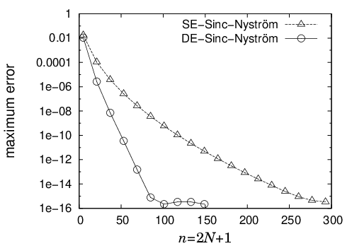
In the SE case, the assumptions in Theorem 3.3 are fulfilled with $\alpha=1$ (note that $g$ , $\mu$ , and $k$ is bounded) and $d=\piup-\epsilon\simeq 3.14$ (note that $d<\piup$ ). In the DE case, the assumptions in Theorem 4.2 are fulfilled with $\alpha=1$ (as in the SE case) and $d=\piup/2-\epsilon\simeq 1.57$ (note that $d<\piup/2$ ). The schemes were implemented with these values for parameters $\alpha$ and $d$ . The errors were investigated on $999$ equally spaced points in $[0,\,1]$ , and their maximum is indicated in Figure 2 by the label “maximum error.” We can observe the theoretical rates; $\Order(\exp(-c\sqrt{N}))$ in the SE-Sinc-Nyström method, and $\Order(\exp(-c^{\prime}N/\log N))$ in the DE-Sinc-Nyström method. Both methods converge exponentially, but DE’s rate is much higher than SE’s rate.

In the next example, there is a pole at $t=-1$ , which affects the DE case.

Example 2

Consider the following equation [7, Example 3]

u^{\prime}(t)=\frac{1}{1+t}-\frac{\left(2+t\log(1+t)\right)\log(1+t)}{2}+u(t)+\int_{0}^{t}\frac{t}{r+1}u(r)\,\mathrm{d}r,\quad 0\leq t\leq 1,

with $u(0)=0$ . The exact solution is $u(t)=\log(1+t)$ .

In the SE case, the assumptions in Theorem 3.3 are fulfilled with $\alpha=1$ and $d=\piup-\epsilon\simeq 3.14$ (as in Example 1). In the DE case, we define $Z$ as

Z=\frac{\piup}{\log 2}\sqrt{\frac{2}{1+\sqrt{1+(2\piup/\log 2)^{2}}}}.

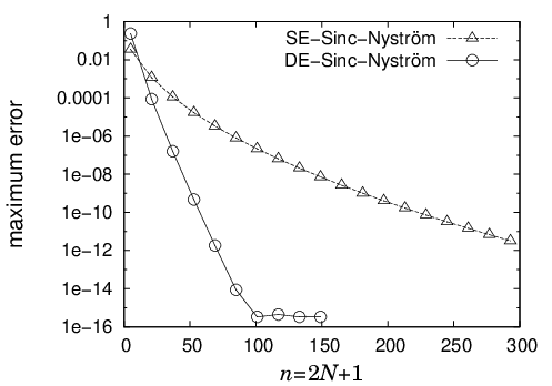
Then, the assumptions in Theorem 4.2 are fulfilled with $\alpha=1$ (as in Example 1) and $d=\arctan(Z)-\epsilon\simeq 1.11$ (note that $g(\psi^{\text{\tiny{\rm DE}}}(\zeta))$ and $k(z,\psi^{\text{\tiny{\rm DE}}}(\zeta))$ is not analytic at $\zeta=\arcsinh(\pm\mathrm{i}\,-\log(2)/\piup)$ ). The errors were investigated in the same way as in Example 1, and are shown in Figure 2. The graph shows the theoretical rates.

Refer to caption — Figure 1: Errors in Example 1.

The next example is more difficult because of a weak singularity at the origin.

Example 3

Consider the following equation

u^{\prime}(t)=\frac{1}{2\sqrt{t}}-tu(t)+\int_{0}^{t}\sqrt{\frac{t}{r}}u(r)\,\mathrm{d}r,\quad 0\leq t\leq 1,

with $u(0)=0$ . The exact solution is $u(t)=\sqrt{t}$ .

In the SE case, the assumptions in Theorem 3.3 are fulfilled with $\alpha=1/2$ (note that $g(t)Q(t)=t^{1/2}(1-t)/2\in\mathbf{L}_{1/2}(\mathscr{D})$ ) and $d=\piup-\epsilon\simeq 3.14$ (as in Example 1). In the DE case, the assumptions in Theorem 4.2 are fulfilled with $\alpha=1/2$ (as in the SE case) and $d=\piup/2-\epsilon\simeq 1.57$ (as in Example 1). The errors are shown in Figure 4, which shows the theoretical rates in this case as well.

The next example is even more difficult because of the infinite singular points distributed around the endpoints.

Example 4

Let $p(t)=\sin(4\arctanh t)$ and $q(t)=\cos(4\arctanh t)+\cosh(\piup)$ , and consider the following equation

	$\displaystyle u^{\prime}(t)$	$\displaystyle=-t\sqrt{\frac{q(t)}{1-t^{2}}}-\frac{2p(t)}{\sqrt{(1-t^{2})q(t)}}+\sqrt{(3+t^{2})(1-t^{2})}u(t)$
		$\displaystyle\quad+\int_{0}^{t}2\sqrt{\frac{3+t^{2}}{1-r^{2}}}\left\{r+\frac{p(r)}{q(r)}\right\}u(r)\,\mathrm{d}r,\quad-1\leq t\leq 1,$

with $u(-1)=0$ . The exact solution is $u(t)=\sqrt{(1-t^{2})q(t)}$ .

In the SE case, the assumptions in Theorem 3.3 are fulfilled with $\alpha=1/2$ and $d=\piup/2-\epsilon\simeq 1.57$ (as in Example 3). In contrast, in the DE case, the assumptions in Theorem 4.2 are not fulfilled for any $d>0$ (although $\alpha=1/2$ can be found as in Example 3), and we do not expect to attain $\Order(\exp(-c^{\prime}N/\log N))$ . However, according to Tanaka et al. [15], the DE-Sinc indefinite integration still converges with a rate similar to that of SE if we set $d=\arcsin((\piup/2-\epsilon)/\piup)\simeq 0.523$ . The errors are shown in Figure 4, and the two methods converge at similar rates.

In the final example, similar to Example 1, all functions in the equation are entire functions.

Example 5

Consider the following equation [16]

\displaystyle u^{\prime}(t)

\displaystyle=\cos t+\frac{\rme^{t}}{5}\left\{\rme^{2t}(\cos t-2\sin t)-1\right\}+\int_{0}^{t}\rme^{t+2r}u(r)\,\mathrm{d}r,\quad 0\leq t\leq 1,

with $u(0)=0$ . The exact solution is $u(t)=\sin t$ .

The assumptions in Theorems 3.3 and 4.2 are fulfilled with the same $\alpha$ and $d$ as those of Example 1. The results of the SE-Sinc-Nyström method and DE-Sinc-Nyström method are shown in Figure 5, with the results of the postprocessing PGFE method [16]. Note that the horizontal axis in Figure 5 is a logarithmic scale axis. The convergence rate of the postprocessing PGFE method is polynomial: $\Order(N^{-4})$ , whereas those of the two Sinc-Nyström methods are exponential. For this reason, the two Sinc-Nyström methods eventually overtake the postprocessing PGFE method.

7 Concluding remarks

A Sinc-Nyström method for (1.1) was developed by Zarebnia [7] (called the SE-Sinc-Nyström method in this paper), for which there remain two points to be discussed. First, the convergence rate of the method was suggested as $\Order(\exp(-c\sqrt{N}))$ , but not proved. Second, the regularity of solution $u$ is necessary for implementation, although $u$ is an unknown function to be determined. For the first point, this paper showed by theoretical analysis that the convergence rate is in fact $\Order(\exp(-c\sqrt{N}))$ . For the second point, this paper showed by theoretical analysis that the regularity of solution $u$ can be determined from the known functions $g$ , $\mu$ , and $k$ .

In addition, this paper proposed a new method called the DE-Sinc-Nyström method by replacing the variable transformation in the SE-Sinc-Nyström method. By a theoretical analysis, this paper showed that $\Order(\exp(-c^{\prime}N/\log N))$ can be attained by the DE-Sinc-Nyström method, and also showed the same result as above on the second point (the regularity of $u$ ).

As explained in Remark 3, the invertibility of the coefficient matrix of the resulting linear system was proved in this paper, but uniform-boundedness of the norm of the matrix was not proved. The latter point will be investigated on another occasion. Generalization of the presented methods for nonlinear Volterra integro-differential equations is also considered as a future work.

References

[1] X.-Q. Zhao, Dynamical Systems in Population Biology, Springer-Verlag, New York, 2003.
[2] A. Makroglou, Integral equations and actuarial risk management: some models and numerics, Math. Model. Anal. 8 (2003) 143–154.
[3] S. Shaw, J. Whiteman, Optimal long-time $L_{p}(0,T)$ stability and semidiscrete error estimates for the Volterra formulation of the linear quasistatic viscoelasticity problem, Numer. Math. 88 (2001) 743–770.
[4] H. Brunner, Collocation Methods for Volterra Integral and Related Functional Differential Equations, Cambridge University Press, Cambridge, 2004.
[5] H. Brunner, The numerical analysis of functional integral and integro-differential equations of Volterra type, Acta Numer. 13 (2004) 55–145.
[6] T. A. Driscoll, Automatic spectral collocation for integral, integro-differential, and integrally reformulated differential equations, J. Comput. Phys. 229 (2010) 5980–5998.
[7] M. Zarebnia, Sinc numerical solution for the Volterra integro-differential equation, Commun. Nonlinear Sci. Numer. Simul. 15 (2010) 700–706.
[8] M. Mori, M. Sugihara, The double-exponential transformation in numerical analysis, J. Comput. Appl. Math. 127 (2001) 287–296.
[9] M. Sugihara, T. Matsuo, Recent developments of the Sinc numerical methods, J. Comput. Appl. Math. 164/165 (2004) 673–689.
[10] S. Haber, Two formulas for numerical indefinite integration, Math. Comput. 60 (1993) 279–296.
[11] M. Muhammad, M. Mori, Double exponential formulas for numerical indefinite integration, J. Comput. Appl. Math. 161 (2003) 431–448.
[12] K. Tanaka, M. Sugihara, K. Murota, Function classes for successful DE-Sinc approximations, Math. Comput. 78 (2009) 1553–1571.
[13] T. Okayama, T. Matsuo, M. Sugihara, Error estimates with explicit constants for Sinc approximation, Sinc quadrature and Sinc indefinite integration, Numer. Math. 124 (2013) 361–394.
[14] H. Brunner, High-order methods for the numerical solution of Volterra integro-differential equations, J. Comput. Appl. Math. 15 (1986) 301–309.
[15] K. Tanaka, T. Okayama, T. Matsuo, M. Sugihara, DE-Sinc methods have almost the same convergence property as SE-Sinc methods even for a family of functions fitting the SE-Sinc methods. Part II: Indefinite integration, Numer. Math. 125 (2013) 545–568.
[16] T. Lin, Y. Lin, M. Rao, S. Zhang, Petrov–galerkin methods for linear volterra integro-differential equations, SIAM J. Numer. Anal. 38 (2000) 937–963.
[17] T. Okayama, T. Matsuo, M. Sugihara, Theoretical analysis of Sinc-Nyström methods for Volterra integral equations, Math. Comput. 84 (2015) 1189–1215.
[18] M. Kolk, A. Pedas, G. Vainikko, High-order methods for Volterra integral equations with general weak singularities, Numer. Funct. Anal. Optim. 30 (2009) 1002–1024.
[19] A. Pedas, G. Vainikko, On the regularity of solutions to integral equations with nonsmooth kernels on a union of open intervals, J. Comput. Appl. Math. 229 (2009) 440–451.
[20] K. E. Atkinson, The Numerical Solution of Integral Equations of the Second Kind, Cambridge University Press, Cambridge, 1997.
[21] F. Stenger, Numerical Methods Based on Sinc and Analytic Functions, Springer-Verlag, New York, 1993.