Fokker-Planck Equations for Stochastic Dynamical Systems with Symmetric Lévy Motions

T. Gao¹¹ 1 Department of Applied Mathematics, Illinois Institute of Technology, Chicago, IL 60616 (tinggao0716@gmail.com). J. Duan²² 2 Department of Applied Mathematics, Illinois Institute of Technology, Chicago, IL 60616 (duan@iit.edu). ⁴⁴ 4 Institute for Pure and Applied Mathematics, University of California, Los Angeles, CA 90095 X. Li³³ 3 Corresponding author. Department of Applied Mathematics, Illinois Institute of Technology, Chicago, IL 60616 (lix@iit.edu).

Abstract

The Fokker-Planck equations for stochastic dynamical systems, with non-Gaussian $\alpha-$ stable symmetric Lévy motions, have a nonlocal or fractional Laplacian term. This nonlocality is the manifestation of the effect of non-Gaussian fluctuations. Taking advantage of the Toeplitz matrix structure of the time-space discretization, a fast and accurate numerical algorithm is proposed to simulate the nonlocal Fokker-Planck equations, under either absorbing or natural conditions. The scheme is shown to satisfy a discrete maximum principle and to be convergent. It is validated against a known exact solution and the numerical solutions obtained by using other methods. The numerical results for two prototypical stochastic systems, the Ornstein-Uhlenbeck system and the double-well system are shown.

keywords

Non-Gaussian noise;

\alpha-

stable symmetric Lévy motion; fractional Laplacian operator; Fokker-Planck equation; maximum principle, convergence, Toeplitz matrix.

AMS

60H10, 60G17, 60G52, 65M12

1 Introduction

The Fokker-Planck (FP) equations for stochastic dynamical systems [13, 12] describe the time evolution for the probability density of solution paths. When the noise in a system is Gaussian (i.e., in terms of Brownian motion), the corresponding Fokker-Planck equation is a differential equation. The Fokker-Planck equations are widely used to investigate stochastic dynamics in physical, chemical and biological systems.

However, the noise is often non-Gaussian [25], e.g., in terms of $\alpha-$ stable Lévy motions. The corresponding Fokker-Planck equation has an integral term and is a differential-integral equation. In fact, this extra term is an integral over the whole state space and thus represents a nonlocal effect caused by the non-Gaussianity of the noise.

A Brownian motion is a Gaussian stochastic process, characterized by its mean or drift vector (taken to be zero for convenience), and a diffusion or covariance matrix.

A Lévy process $L_{t}$ on $\mathbb{R}^{n}$ is a non-Gaussian stochastic process. It is characterized by a drift vector $b\in\mathbb{R}^{n}$ (taken to be zero for convenience), a Gaussian covariance matrix $A$ , and a non-negative Borel measure $\nu$ , defined on $({\mathbb{R}}^{n},\mathcal{B}({\mathbb{R}}^{n}))$ and concentrated on ${\mathbb{R}}^{n}\setminus\{0\}$ . The measure $\nu$ satisfies the condition

\int_{{\mathbb{R}}^{n}\setminus\{0\}}(y^{2}\wedge 1)\;\nu(dy)<\infty,

where $a\wedge b=\min\{a,b\}$ , or equivalently

\int_{{\mathbb{R}}^{n}\setminus\{0\}}\frac{y^{2}}{1+y^{2}}\;\nu(dy)<\infty.

This measure $\nu$ is the so called Lévy jump measure of the Lévy process $L_{t}$ . We also call $(b,A,\nu)$ the generating triplet [3, 21].

In this paper, we consider stochastic differential equations (SDEs) with a special class of Lévy processes, the $\alpha$ -stable symmetric Lévy motions. The corresponding Fokker-Planck equations (for the evolution of the probability density function of the solution) contain a nonlocal term, i.e., the fractional Laplacian term, which quantifies the non-Gaussian effect. It is hardly possible to have analytical solutions for these nonlocal Fokker-Planck equations even for simple systems. We thus consider numerical simulation for these nonlocal equations, either on a bounded domain or a unbounded domain. Due to the nonlocality, however, the ‘boundary’ condition needs to be prescribed on the entire exterior domain. A recently developed nonlocal vector calculus has provided sufficient conditions for the well-posedness of the initial-boundary value problems on this type of nonlocal diffusion equations with volume constraints. See the review paper [8].

A few authors have considered numerical simulations of reaction-diffusion type partial differential equations with a (formal) fractional Laplacian operator. They impose a boundary condition only on the boundary of a bounded set (not on the entire exterior set as we do here); see [10], [18, Eqs. (10) and (11)], [5, §3], [19], [26, Eq. (2)] and references therein. The domain of definition of the fractional Laplacian operator in these papers consists of certain functions with prescribed values on the boundary. However, the domain of definition of the fractional Laplacian operator in our present paper consists of certain functions with prescribed values on the entire exterior domain. Thus, the fractional Laplacian operator in the present paper is different from that in [10, 18, 5, 19, 26], as the domains of definition are different. Note that the exterior boundary condition is required for understanding probability density evolution. Recently, discontinuous and continuous Galerkin methods have been developed for the volume-constrained nonlocal diffusion problems and their error analysis is given in [8] and the references therein. To our knowledge, the work [9] is closely related to our work, where the authors of [9] have shown the well-posedness, the maximum principle, conservation and dispersion relations for a class of nonlocal convection-diffusion equations with volume constraints. A finite difference scheme is also presented in [9], which maintains the maximum principle when suitable conditions are met. Compared with this paper, the difference is that the jump processes considered in [9] are nonsymmetric and of finite-range.

This paper is organized as follows. In section 2, we present the nonlocal Fokker-Planck equation for a SDE with $\alpha-$ stable symmetric Lévy motion and then devise a numerical discretization scheme, with either the absorbing or natural condition. For simplicity, we consider scalar SDEs. The description and analysis of the numerical schemes are presented in section 3 and section 4, respectively. The numerical experiments are conducted in section 5. The paper ends with some discussions in section 6.

2 Fokker-Planck equations for SDEs with Lévy motions

Consider a scalar SDE

{\rm d}X_{t}=f(X_{t})\,{\rm d}t+{\rm d}L_{t},X_{0}=x_{0},

(1)

where $f$ is a given deterministic vector field, the scalar Lévy process $L_{t}$ has the generating triplet $(0,d,\varepsilon\nu_{\alpha})$ , with diffusion constant $d\geq 0$ and the $\alpha-$ stable symmetric jump measure

\nu_{\alpha}({\rm d}y)=C_{\alpha}|y|^{-(1+\alpha)}\,{\rm d}y.

The constant $C_{\alpha}$ is defined as $\displaystyle{C_{\alpha}=\frac{\alpha}{2^{1-\alpha}\sqrt{\pi}}\frac{\Gamma(\frac{1+\alpha}{2})}{\Gamma(1-\frac{\alpha}{2})}}$ . The non-Gaussianity index $\alpha\in(0,2)$ and the intensity constant is $\varepsilon$ . For more information on $\alpha-$ stable Lévy motions, see [1, 7, 22].

The FP equation for the distribution of the conditional probability density $p(x,t)=p(x,t|x_{0},0)$ , i.e., the probability of the process $X_{t}$ has value $x$ at time $t$ given it had value $x_{0}$ at time $0$ , is given by [3, 22, 1, 2]

p_{t}=-(f(x)\;p)_{x}+\frac{1}{2}dp_{xx}+\varepsilon[k_{\alpha}(-\Delta)^{\frac{\alpha}{2}}]^{*}p.

(2)

Note that the integro-differential part $k_{\alpha}(-\Delta)^{\frac{\alpha}{2}}$ is symmetric on $L^{2}({\mathbb{R}})$ (see [1]). Thus,

\partial_{t}p=-\partial_{x}[f(x)\;p]+\frac{d}{2}\partial_{xx}p+\varepsilon k_{\alpha}(-\Delta)^{\frac{\alpha}{2}}p,

(3)

where

k_{\alpha}\triangleq\int_{{\mathbb{R}}\setminus\{0\}}(\cos y-1)\;\nu_{\alpha}(dy)<0.

This equation may be rewritten as

	$\displaystyle p_{t}$	$\displaystyle=$	$\displaystyle-(f(x)\;p)_{x}+\frac{1}{2}dp_{xx}$		(4)
		$\displaystyle+$	$\displaystyle\int_{{\mathbb{R}}\setminus\{0\}}[p(x+y,t)-p(x,t)-I_{\{\|y\|<1\}}\;y\;p_{x}(x,t)]\;\varepsilon\nu_{\alpha}({\rm d}y).$		(4)

2.1 Auxiliary Conditions

We consider two kinds of auxiliary conditions, the absorbing nonlocal ”Dirichlet” condition and natural far-field condition.

The absorbing condition on the finite interval $(a,b)$ states that the probability of finding “particles” $X_{t}$ outside $(a,b)$ is zero:

p(x,t)=0,\;\;\mbox{ for }x\notin(a,b).

(5)

The natural far-field conditions in this work are specified as follows: the domain is the whole real line ${\mathbb{R}}=(-\infty,\infty)$ ,

p(x,t)\rightarrow 0,\quad\text{ as }|x|\rightarrow\infty,

(6)

and the decay rate is fast enough to ensure

\int_{-\infty}^{\infty}p(x,t)\,{\rm d}x=1,\quad\text{for all }t\geq 0.

(7)

3 Numerical Methods

For clarity and without losing generality, in the following, we present the numerical algorithms the case of $(a,b)=(-1,1)$ with the absorbing condition (5).

Noting that the absorbing condition dictates that $p$ vanish outside $(-1,1)$ , we can simplify Eq. (4) by decomposing the integral into three parts $\int_{{\mathbb{R}}}=\int_{-\infty}^{-1-x}+\int_{-1-x}^{1-x}+\int_{1-x}^{\infty}$ and analytically evaluating the first and third integrals

	$\displaystyle p_{t}$	$\displaystyle=$	$\displaystyle-(f(x)p)_{x}+\frac{d}{2}p_{xx}-\frac{\varepsilon C_{\alpha}}{\alpha}\left[\frac{1}{(1+x)^{\alpha}}+\frac{1}{(1-x)^{\alpha}}\right]p$		(8)
			$\displaystyle+\varepsilon C_{\alpha}\int_{-1-x}^{1-x}\frac{p(x+y,t)-p(x,t)}{\|y\|^{1+\alpha}}\;{\rm d}y,$		(8)

for $x\in(-1,1)$ ; and $p(x,t)=0$ for $x\notin(-1,1)$ . We have dropped the integral $\displaystyle{\int_{\mathbb{R}}\frac{I_{\{|y|<1\}}(y)\,y}{|y|^{1+\alpha}}\;{\rm d}y}$ , since the principal value integral vanishes and we find it does not improve the accuracy of the numerical integration of the singular integral in (4) [11].

Next, we describe a numerical method for discretizing the Fokker-Planck equation (8), a time-dependent integro-differential equation. For the spatial derivatives, the advection term $-(f(x)p)_{x}$ is discretized by the third-order WENO method provided in [17] and [16]) while the diffusion term is approximated by the second-order central differencing scheme. The numerical scheme for the remaining nonlocal integral term in (8) is presented in detail as follows.

Let’s divide the interval $[-2,2]$ in space into $4J$ sub-intervals and define $x_{j}=jh$ for $-2J\leq j\leq 2J$ integer, where $h=1/J$ . We denote the numerical solution of $p$ at $(x_{j},t)$ by $P_{j}$ . Then, using a modified trapezoidal rule for approximating the singular integral [11], we obtain the semi-discrete equation

\begin{split}\dfrac{{\rm d}P_{j}}{{\rm d}t}=&C_{h}\frac{P_{j-1}-2P_{j}+P_{j+1}}{h^{2}}-[(fP)_{x,j}^{+}+(fP)_{x,j}^{-}]\\ &-\frac{\varepsilon C_{\alpha}}{\alpha}\left[\frac{1}{(1+x_{j})^{\alpha}}+\frac{1}{(1-x_{j})^{\alpha}}\right]P_{j}+\varepsilon C_{\alpha}h\sum^{J-j}_{k=-J-j,k\neq 0}\!\!\!\!\!\!\!\!\!{{}^{\prime\prime}}\;{\frac{P_{j+k}-P_{j}}{|x_{k}|^{1+\alpha}}},\end{split}

(9)

for $0<\alpha<2$ and $j=-J+1,\cdots,-2,-1,0,1,2,\cdots,J-1$ , where the constant $C_{h}$ $\displaystyle{=\frac{d}{2}-\varepsilon C_{\alpha}\zeta(\alpha-1)h^{2-\alpha}}$ . $\zeta$ is the Riemann zeta function. The $\pm$ superscripts denote the global Lax-Friedrichs flux splitting defined as $(fP)^{\pm}=\frac{1}{2}(fP\pm\alpha P)$ with $\alpha=\max_{x}|f(x)|$ . The summation symbol $\sum{{}^{\prime\prime}}$ means that the quantities corresponding to the two end summation indices are multiplied by $1/2$ . The absorbing condition requires that the values of $P_{j}$ vanish if the index $|j|\geq J$ .

The first-order derivatives $(fP)_{x,j}^{+}$ and $(fP)_{x,j}^{-}$ are approximated by the third-order WENO scheme [16]. The approximation to $\varphi_{x}(x_{j})$ on left-biased stencil $\{x_{k},k=j-2,j-1,j,j+1\}$ is given by

\varphi_{x,j}^{+}=\frac{1}{2h}(\Delta^{+}\varphi_{j-1}+\Delta^{+}\varphi_{j})-\frac{\omega_{-}}{2h}(\Delta^{+}\varphi_{j-2}-2\Delta^{+}\varphi_{j-1}+\Delta^{+}\varphi_{j})

where

\omega_{-}=\frac{1}{1+2r_{-}^{2}},\ \ \ \ r_{-}=\frac{\delta+(\Delta^{-}\Delta^{+}\varphi_{j-1})^{2}}{\delta+(\Delta^{-}\Delta^{+}\varphi_{j})^{2}}.

Here $\delta=10^{-6}$ is used to prevent the denominators from being zero. The approximation to $\varphi_{x}(x_{j})$ on right-biased stencil $\{x_{k},k=j-1,j,j+1,j+2\}$ is given by

\varphi_{x,j}^{-}=\frac{1}{2h}(\Delta^{+}\varphi_{j-1}+\Delta^{+}\varphi_{j})-\frac{\omega_{+}}{2h}(\Delta^{+}\varphi_{j+1}-2\Delta^{+}\varphi_{j}+\Delta^{+}\varphi_{j-1})

where

\omega_{+}=\frac{1}{1+2r_{+}^{2}},\ \ \ \ r_{+}=\frac{\delta+(\Delta^{-}\Delta^{+}\varphi_{j+1})^{2}}{\delta+(\Delta^{-}\Delta^{+}\varphi_{j})^{2}}.

Note that $\Delta^{+}\psi_{j}=\psi_{j+1}-\psi_{j}$ , $\Delta^{-}\psi_{j}=\psi_{j}-\psi_{j-1}$ and $\varphi_{-J-1}^{\pm}=\varphi_{-J}^{\pm}=\varphi_{J}^{\pm}=\varphi_{J+1}^{\pm}=0.$

For time evolution, we adopt a third-order total variation diminishing(TVD) Runge-Kutta method given in [23]. In particular, for the ordinary differential equation(ODE) $\dfrac{{\rm d}u}{{\rm d}t}=R(u)$ , the method can be written as

\begin{split}U^{(1)}&=U^{n}+\Delta tR(U^{n}),\\ U^{(2)}&=\frac{3}{4}U^{n}+\frac{1}{4}U^{(1)}+\frac{1}{4}\Delta tR(U^{(1)}),\\ U^{n+1}&=\frac{1}{3}U^{n}+\frac{2}{3}U^{(2)}+\frac{2}{3}\Delta tR(U^{(2)}),\end{split}

(10)

where $U^{n}$ denotes the numerical solution of $u$ at time $t=t_{n}$ .

The computational cost of the proposed numerical method is dominated by the summation term in the scheme (9). If the right-hand side of (9) is written in matrix-vector multiplication form, the matrix corresponding to the summation term would be dense but is Toeplitz. The Toeplitz-vector products can be computed fast with $O(J\log J)$ number of operation counts instead of $O(J^{2})$ , where the matrix dimension is $O(J)$ [14]. We find that the fast algorithm is crucial in solving the Fokker-Planck equation for the natural far-field condition.

Remark 1.

For the natural far-field condition (6), the semi-discrete equation corresponding to (4) becomes

\begin{split}\dfrac{{\rm d}P_{j}}{{\rm d}t}=&C_{h}\frac{P_{j-1}-2P_{j}+P_{j+1}}{h^{2}}-[(fP)_{x,j}^{+}+(fP)_{x,j}^{-}]+\varepsilon C_{\alpha}h\sum^{J-j}_{k=-J-j,k\neq 0}\!\!\!\!\!\!\!\!\!{{}^{\prime\prime}}\;{\frac{P_{j+k}-P_{j}}{|x_{k}|^{1+\alpha}}},\end{split}

(11)

where $J=L/h$ and $L\gg 1$ . Unlike the case of the absorbing condition, the values of the density outside the computational domain $(-L,L)$ are unknown for the natural condition. We perform numerical calculations on increasing larger intervals $(a,b)=(-L,L)$ until the results are convergent.

4 Analysis of our numerical scheme

The numerical analysis for linear convection-diffusion equations are well-known and have been described in many classic textbooks. In this section, we perform the analysis on the nonlocal term in (4) due to the $\alpha$ -stable process by requiring neither Gaussian diffusion nor the deterministic drift be present. i.e., $d=0$ and $f\equiv 0$ . We now analyze the numerical schemes proposed in §3, by examining its discrete maximal principle, stability and convergence.

4.1 Discrete Maximum Principle

First, we examine the discrete maximum principle of the scheme (9) with the absorbing nonlocal Dirichlet condition (5). Due to the positivity of the probability density function and the vanishing condition (5) outside the domain, the maximum principle states that the solution in the domain lies within the interval $[0,M]$ , where $M$ is the maximum value of the initial probability function.

Proposition 1.

When both $d$ and $f$ vanish, the scheme (9) corresponding to the absorbing condition with forward Euler for time integration satisfies the discrete maximum principle, i.e., $0\leq P_{j}^{0}\leq M$ for all $j$ ’s implies $0\leq P_{j}^{n}\leq M$ for all $n>0$ and $j$ ’s, if the following inequality holds

\frac{\Delta t}{h^{\alpha}}\leq\frac{1}{2\varepsilon C_{\alpha}\left[1+\frac{1}{\alpha}-\zeta(\alpha-1)\right]}.

(12)

Proof.

We only need to show $0\leq P_{j}^{n+1}\leq M$ given $0\leq P_{j}^{n}\leq M$ . Applying the explicit Euler to the semi-discrete scheme (9), we have

\begin{split}P_{j}^{n+1}=&P_{j}^{n}-\Delta t\varepsilon C_{\alpha}\zeta(\alpha-1)h^{-\alpha}(P_{j-1}^{n}-2P_{j}^{n}+P_{j+1}^{n})\\ &-\frac{\Delta t\varepsilon C_{\alpha}}{\alpha}\left[\frac{1}{(1+x_{j})^{\alpha}}+\frac{1}{(1-x_{j})^{\alpha}}\right]P_{j}^{n}+\Delta t\varepsilon C_{\alpha}h\sum^{k=J-j}_{k=-J-j,k\neq 0}\!\!\!\!{{}^{\prime\prime}}\;{\frac{P_{j+k}^{n}-P_{j}^{n}}{|x_{k}|^{1+\alpha}}}\\ =&\left\{1+\frac{2\Delta t\varepsilon C_{\alpha}\zeta(\alpha-1)}{h^{\alpha}}-\frac{\Delta t\varepsilon C_{\alpha}}{\alpha}\left[\frac{1}{(1+x_{j})^{\alpha}}+\frac{1}{(1-x_{j})^{\alpha}}\right]\right.\\ &-\Delta t\varepsilon C_{\alpha}h\left.\sum^{k=J-j}_{k=-J-j,k\neq 0}\!\!\!\!{{}^{\prime\prime}}\;{\frac{1}{|x_{k}|^{1+\alpha}}}\right\}P_{j}^{n}-\frac{\Delta t\varepsilon C_{\alpha}\zeta(\alpha-1)}{h^{\alpha}}\left(P_{j-1}^{n}+P_{j+1}^{n}\right)\\ &+\Delta t\varepsilon C_{\alpha}h\sum^{k=J-j}_{k=-J-j,k\neq 0}\!\!\!\!{{}^{\prime\prime}}\;{\frac{P_{j+k}^{n}}{|x_{k}|^{1+\alpha}}},\end{split}

(13)

where $J=1/h$ . Noting $\zeta(x)$ is negative for $-1<x<1$ , the coefficients of non-diagonal terms $P_{m}^{n}$ with $m\neq j$ are all positive. Thus,

\begin{split}P_{j}^{n+1}\leq&\left\{1+\frac{2\Delta t\varepsilon C_{\alpha}\zeta(\alpha-1)}{h^{\alpha}}-\frac{\Delta t\varepsilon C_{\alpha}}{\alpha}\left[\frac{1}{(1+x_{j})^{\alpha}}+\frac{1}{(1-x_{j})^{\alpha}}\right]\right.\\ &-\Delta t\varepsilon C_{\alpha}h\left.\sum^{k=J-j}_{k=-J-j,k\neq 0}\!\!\!\!{{}^{\prime\prime}}\;{\frac{1}{|x_{k}|^{1+\alpha}}}\right\}M\\ &+\left[-2\frac{\Delta t\varepsilon C_{\alpha}\zeta(\alpha-1)}{h^{\alpha}}+\Delta t\varepsilon C_{\alpha}h\sum^{k=J-j}_{k=-J-j,k\neq 0}\!\!\!\!{{}^{\prime\prime}}\;{\frac{1}{|x_{k}|^{1+\alpha}}}\right]M\leq M,\end{split}

(14)

provided that

1+\frac{2\Delta t\varepsilon C_{\alpha}\zeta(\alpha-1)}{h^{\alpha}}-\frac{\Delta t\varepsilon C_{\alpha}}{\alpha}\left[\frac{1}{(1+x_{j})^{\alpha}}+\frac{1}{(1-x_{j})^{\alpha}}\right]-\Delta t\varepsilon C_{\alpha}h\sum^{k=J-j}_{k=-J-j,k\neq 0}\!\!\!\!{{}^{\prime\prime}}\;{\frac{1}{|x_{k}|^{1+\alpha}}}\geq 0.

(15)

Similarly, when the condition (15) is met, we can also prove that $P_{j}^{n+1}\geq 0$ given $P_{j}^{n}\geq 0$ for all $j$ , because all coefficients for the elements of $P^{n}$ in (13) are non-negative.

Next, we derive a sufficient condition (12) that guarantees the inequality (15). We have the following estimate

\begin{split}&\Delta t\varepsilon C_{\alpha}h\sum^{k=J-j}_{k=-J-j,k\neq 0}\!\!\!\!{{}^{\prime\prime}}\;{\frac{1}{|x_{k}|^{1+\alpha}}}+\frac{\Delta t\varepsilon C_{\alpha}}{\alpha}\left[\frac{1}{(1+x_{j})^{\alpha}}+\frac{1}{(1-x_{j})^{\alpha}}\right]\\ &=\Delta t\varepsilon C_{\alpha}\left[h\sum^{k=J-j}_{k=-J-j,k\neq 0}\!\!\!\!{{}^{\prime\prime}}\;{\frac{1}{|x_{k}|^{1+\alpha}}}+\int_{-\infty}^{-1-jh}\frac{1}{|y|^{1+\alpha}}dy+\int_{1-jh}^{\infty}\frac{1}{|y|^{1+\alpha}}dy\right]\\ &\leq\Delta t\varepsilon C_{\alpha}\left[\frac{2h}{h^{1+\alpha}}+\int_{-1-jh+\frac{h}{2}}^{-h}\frac{1}{|y|^{1+\alpha}}dy+\int_{h}^{1-jh-\frac{h}{2}}\frac{1}{|y|^{1+\alpha}}dy+\int_{-\infty}^{-1-jh}\frac{1}{|y|^{1+\alpha}}dy+\int_{1-jh}^{\infty}\frac{1}{|y|^{1+\alpha}}dy\right]\\ &\leq\Delta t\varepsilon C_{\alpha}\left[\frac{2}{h^{\alpha}}+2\int_{h}^{\infty}\frac{1}{y^{1+\alpha}}dy\right]=\Delta t\varepsilon C_{\alpha}\left[\frac{2}{h^{\alpha}}\left(1+\frac{1}{\alpha}\right)\right]\end{split}

(16)

where $x_{j}=jh$ .

From the estimate (16), the inequality (15) holds if

\Delta t\varepsilon C_{\alpha}\left[\frac{2}{h^{\alpha}}\left(1+\frac{1}{\alpha}\right)-\frac{2\zeta(\alpha-1)}{h^{\alpha}}\right]=\frac{\Delta t}{h^{\alpha}}2\varepsilon C_{\alpha}\left[1+\frac{1}{\alpha}-\zeta(\alpha-1)\right]\leq 1,

(17)

which is equivalent to the condition (12). ∎

Next, we turn to the scheme for the natural condition.

Proposition 2.

When both $d$ and $f$ vanish, the scheme (11) corresponding to the natural condition with forward Euler for time integration satisfies the discrete maximum principle, i.e., $0\leq P_{j}^{0}\leq M$ for all $j$ ’s implies $0\leq P_{j}^{n}\leq M$ for all $n>0$ and $j$ ’s, if the inequality (12) holds.

Proof.

With the explicit Euler method for time integration, Eq. (11) becomes

P_{j}^{n+1}=P_{j}^{n}-\Delta t\varepsilon C_{\alpha}\zeta(\alpha-1)h^{-\alpha}(P_{j-1}^{n}-2P_{j}^{n}+P_{j+1}^{n})+\Delta t\varepsilon C_{\alpha}h\sum^{k=J-j}_{k=-J-j,k\neq 0}\!\!\!\!{{}^{\prime\prime}}\;{\frac{P_{j+k}^{n}-P_{j}^{n}}{|x_{k}|^{1+\alpha}}},

(18)

where $J=L/h$ and $L\gg 1$ . The difference between the discrete equations corresponding to the absorbing condition and natural condition, (13) and (18), is that (18) does not have the term $\displaystyle\frac{\Delta t\varepsilon C_{\alpha}}{\alpha}\left[\frac{1}{(1+x_{j})^{\alpha}}+\frac{1}{(1-x_{j})^{\alpha}}\right]P_{j}^{n}$ .

Similar to the proof of Proposition 1, (18) satisfies discrete maximum principle provided that

1+2\frac{\Delta t\varepsilon C_{\alpha}\zeta(\alpha-1)}{h^{\alpha}}-\Delta t\varepsilon C_{\alpha}h\sum^{k=J-j}_{k=-J-j,k\neq 0}\!\!\!\!{{}^{\prime\prime}}\;{\frac{1}{|x_{k}|^{1+\alpha}}}\geq 0.

(19)

And, a similar estimate

\begin{split}&\Delta t\varepsilon C_{\alpha}h\sum^{k=J-j}_{k=-J-j,k\neq 0}\!\!\!\!{{}^{\prime\prime}}\;{\frac{1}{|x_{k}|^{1+\alpha}}}\leq\Delta t\varepsilon C_{\alpha}\left[\frac{2h}{h^{1+\alpha}}+\int_{-L-jh+\frac{h}{2}}^{-h}\frac{1}{|y|^{1+\alpha}}dy+\int_{h}^{L-jh-\frac{h}{2}}\frac{1}{|y|^{1+\alpha}}dy\right]\\ \leq&\Delta t\varepsilon C_{\alpha}\left[\frac{2}{h^{\alpha}}+2\int_{h}^{\infty}\frac{1}{y^{1+\alpha}}dy\right]=\Delta t\varepsilon C_{\alpha}\left[\frac{2}{h^{\alpha}}\left(1+\frac{1}{\alpha}\right)\right]\end{split}

(20)

leads to the same condition (12) for maximum principle. ∎

Now, we are ready to show that both semi-discrete schemes (9) and (11) with the third-order TVD Runge-Kutta time discretization (10) satisfy the discrete maximum principle.

Proposition 3.

When both $d$ and $f$ vanish, the semi-discrete schemes (9) and (11), corresponding to the absorbing and the natural conditions respectively, with the third-order Runge-Kutta time discretization (10) satisfy the discrete maximum principle, i.e., $0\leq P_{j}^{0}\leq M$ for all $j$ ’s implies $0\leq P_{j}^{n}\leq M$ for all $n>0$ and $j$ ’s, if the inequality (12) holds.

Proof.

Propositions 1 and 2 have shown that the semi-discrete schemes (9) and (11) with the forward Euler time discretization satisfies the discrete maximum principle when the inequality (12) holds. Based on the proof of Proposition 2.1 in [23], the explicit Runge-Kutta method (10) satisfies the maximum principle under the same restriction (12), because it can be written as a convex combination of the operations that satisfy the maximum principle due to Propositions 1 and 2. ∎

Refer to caption — Fig. 1: The dependence of the threshold $\frac{1}{2C_{\alpha}\left[1+\frac{1}{\alpha}-\zeta(\alpha-1)\right]}$ on $\alpha$ with $\varepsilon=1$ .

Remark 2.

It is interesting to note that the condition for the explicit method corresponding to $\alpha$ -stable process (12) limits the ratio of the time step $\Delta t$ to the spatial grid size $h^{\alpha}$ , while the corresponding condition for the Gaussian diffusion term $p_{xx}$ limits the ratio $\Delta t/h^{2}$ . Further, the $\alpha$ -stable process is Gaussian when $\alpha=2$ . The upper bound of the ratio for satisfying the maximum principle, i.e., the value of the constant on the right-hand side of the inequality (12), is plotted for $0<\alpha<2$ in Fig. 1. Surprisingly, the value of the threshold decays from $1$ to $1/2$ as $\alpha$ increases from $0$ to $2$ . To satisfy the maximum principle, we recall the condition for the classic explicit scheme corresponding to the heat equation $p_{t}=\varepsilon p_{xx}$ , the forward Euler in time and the second-order central differencing in space, is $\Delta t/h^{2}<1/2$ , matching the limit of the inequality of (12) as $\alpha$ approaches $2$ . This agreement suggests that the condition (12) might be sharp for satisfying the maximum principle.

4.2 Stability and Convergence

Due to the linearity of the schemes (13) and (18), their stability can be deduced by means of the maximum principle shown in the previous section § 4.1. Therefore, the explicit schemes (13) and (18) are stable when the ratio $\Delta t/h^{\alpha}$ satisfies the condition (12).

Now we explore the convergence condition of the forward Euler scheme (18) for the equation $(\ref{FPE555})$ with the natural far-field condition. Although our proof is for the case where the diffusion $d$ and the drift $f$ are absent, the extension to the cases in which both $d$ and $f$ are present is straightforward. Also, one can easily extend the following proof of convergence result to other different time integration schemes for the semi-discrete equations (9) and (11).

Proposition 4.

The solution $U_{j}^{n}$ to the numerical scheme (18) for the natural far-field condition converges to the analytic solution to (4) for $x_{j}$ in $[-L/2,L/2]$ when the refinement path satisfies (12) and the length of the integration interval $2L$ in (18) tends to $\infty$ .

Proof.

Denote the discretization error by $e_{j}^{n}:=P_{j}^{n}-p(x_{j},t_{n})$ , where $p$ is the analytic solution. Defining the truncation error $T_{j}^{n}$ as the difference between the left-hand and right-hand sides of (18) evaluated at $(x_{j},t_{n})$ when the numerical solution $P_{j}^{n}$ is replaced with the analytic solution $p(x_{j},t_{n})$ divided by $\Delta t$ , the linearity of the equation leads to

e_{j}^{n+1}=e_{j}^{n}-\Delta t\varepsilon C_{\alpha}\zeta(\alpha-1)h^{2-\alpha}\frac{e_{j-1}^{n}-2e_{j}^{n}+e_{j+1}^{n}}{h^{2}}+\Delta t\varepsilon C_{\alpha}h\sum^{k=J-j}_{k=-J-j,k\neq 0}\!\!\!\!\!{{}^{\prime\prime}}\;{\frac{e_{j+k}^{n}-e_{j}^{n}}{|x_{k}|^{1+\alpha}}}-\Delta tT_{j}^{n},

(21)

where $J=L/h$ . The leading-order terms in the truncation error are given by

\begin{split}T_{j}^{n}=&\frac{1}{2}p_{tt}(x_{j},t_{n})\Delta t+\frac{1}{12}\varepsilon C_{\alpha}\zeta(\alpha-1)p_{xxxx}(x_{j},t_{n})h^{4-\alpha}-C\varepsilon\frac{\partial}{\partial y}\left.\left(\frac{p(x_{j}+y,t_{n})}{|y|^{1+\alpha}}\right)\right|_{y=-L-x_{j}}^{y=L-x_{j}}h^{2}\\ &-D\varepsilon\zeta(\alpha-3)p_{xxxx}(x_{j},t_{n})h^{4-\alpha}+\int_{\{-\infty,-L-x_{j}\}\cup\{L-x_{j},\infty\}}\frac{p(x_{j}+y,t)-p(x_{j},t)}{|y|^{1+\alpha}}\,{\rm d}y+\cdots,\end{split}

(22)

where $C$ and $D$ are constants. Thus, the truncation error is uniformly bounded,

|T_{j}^{n}|\leq\bar{T}:=O(\Delta t)+O(h^{2})+O(L^{-\alpha}).

(23)

Using the same argument as in the proof in Proposition 2, under the condition (12), the coefficients of $e_{m}^{n}$ are nonnegative for all $m$ ’s. Denoting $E^{n}=\max_{j}|e_{j}^{n}|$ , we have

E^{n+1}\leq E^{n}+\Delta t\bar{T},\quad\text{then}\quad E^{n}\leq E^{0}+n\Delta t\bar{T}=n\Delta t\bar{T}.

(24)

Therefore, the convergence is proved.

∎

Remark 3.

Because the derivatives of the density function $p$ might be infinite at the boundaries of the domain $(-1,1)$ for the absorbing condition, as shown in next section, the truncation error of the modified trapezoidal rule is not uniformly second-order. The numerical analysis of the convergence for (13) will be studied in future.

5 Numerical results

5.1 Verification

For some special cases, the analytic or exact solutions can be obtained by inspecting the characteristic functions in the form of Fourier Transform ([15]) or series expansion ([4]). We first compare our numerical solution with the exact solution $\displaystyle{p(x,t)=\frac{t}{\pi(t^{2}+x^{2})}}$ for the Cauchy case with the natural far-field condition, which corresponds to the FP equation (3) with $d=0$ , $f=0$ , $\varepsilon=1$ , $\alpha=1$ . To avoid numerical complication of a delta function, we start our numerical computation from time $t=0.01$ by setting the initial condition to be $\displaystyle{p(x,0.01)=\frac{0.01}{\pi(0.01^{2}+x^{2})}}$ and approximating the natural far-field condition by truncating the computational domain to $(-50,50)$ using the numerical scheme given in Eq. (11). Both the exact and the numerical solutions are shown in Fig. 2 at the times $t=0.05,0.01$ and $0.2$ . In the numerical simulations, we have chosen the spatial resolution $h=0.001$ and the time step size $\Delta t=0.5h$ . As the graphs show, the numerical results are indistinguishable from the exact solution, implying our numerical methods produce correct and accurate results.

We also examine the maximum absolute error and the relative error in 2-norm of our numerical solution, defined by $\|\mathbf{e}_{n}\|_{\infty}\equiv\max_{j}|P^{n}_{j}-p(x_{j},t_{n})|$ and $\|\mathbf{e}_{n}\|_{2}/\|(p(x_{j},t_{n}))\|_{2}$ respectively. Here, the error vector $\mathbf{e}_{n}$ is defined as $\mathbf{e}_{n}:=(P^{n}_{j}-p(x_{j},t_{n}))$ , the difference between the numerical solution $(P^{n}_{j})$ and the exact solution $(p(x_{j},t_{n}))$ at the time $t_{n}$ . Figure 3 shows the sizes of the errors of our numerical solutions obtained by using the computational domain $(-50,50)$ , $h=0.001$ and $\Delta t=0.5h$ , as the time increases from $0.01$ to $0.2$ . The absolute error increases initially but levels off quickly as the solution itself becomes small, while the relative error grows linearly in time. Up to time $t=0.2$ , the relative error is small (less than 0.3%).

Next, we check the order of convergence of our numerical methods in space. In theory [24], with the correction term $-\varepsilon C_{\alpha}\zeta(\alpha-1)h^{2-\alpha}$ , the error between the integro-differential term $\varepsilon k_{\alpha}(-\Delta)^{\frac{\alpha}{2}}$ in Eq. (3) and its numerical approximation in Eq. (9) is given by

-\sum\limits_{\mu=1}^{m-1}C_{\mu}\left[\frac{\partial^{2\mu-1}}{\partial y^{2\mu-1}}\left(\left.\frac{p(x+y,t)}{|y|^{1+\alpha}}\right)\right|_{y=-L}^{y=L}\right]h^{2\mu}-\sum\limits_{\mu=2}^{m-1}D_{\mu}\zeta(\alpha+1-2\mu)\frac{\partial^{2\mu}p}{\partial x^{2\mu}}(x,t)\,h^{2\mu-\alpha}+O(h^{2m}),

(25)

where $L\gg|x|$ , and $C_{\mu}$ and $D_{\mu}$ are constants related to $\mu$ .

$h$	$0.1$	$0.1/2$	$0.1/2^{2}$	$0.1/2^{3}$	$0.1/2^{4}$	$0.1/2^{5}$	$0.1/2^{6}$
Error	$1.01$	$0.264$	$0.0554$	$4.23\times 10^{-3}$	$8.41\times 10^{-5}$	$4.13\times 10^{-5}$	$3.93\times 10^{-5}$
Order	$1.94$	$2.25$	$3.71$	$5.65$	$1.03$	$0.0734$

Table 1: The error of the numerical solution of

p(x,t)

at the fixed point

(x,t)=(0.1,0.02)

and the numerical order of convergence for difference sizes of the resolution

h

. The numerical solutions are obtained without Richardson extrapolation.

In Table 1, we provide the computed order of convergence in space using different sizes of $h$ for the Cauchy case $\alpha=1$ with the natural far-field condition, no deterministic driving force $f=0$ and no Gaussian diffusion $d=0$ . The error in the numerical solution is computed with the computational domain $(-L,L)=(-100,100)$ at a fixed point $(x,t)=(0.1,0.02)$ by comparing with the known exact solution $p(0.1,0.02)$ and, again, the initial data is taken from the exact solution at time $t=0.01$ . The numerical order of convergence is calculated from the formula $\log_{2}|e(h)/e(h/2)|$ , where $e(h)$ denotes the error at the point $(x,t)=(0.1,0.02)$ with the spatial resolution $h$ .

The results in Table 1 shows that, for relatively large or moderate sizes of $h$ , the order of convergence is either close to or better than two. Second-order convergence is expected from the theory (25). The higher orders of convergence shown in Table 1 can be explained as follows. First, for $\alpha=1$ , the second summation in the quadrature error (25) vanishes due to $\zeta(-2)=\zeta(-4)=\cdots=0$ . Second, the coefficients in the terms of the first summation in (25) are small because the unknown function $p$ and its spatial derivatives vanish at the infinity and are small when $L$ is large. However, the error in the numerical solution ceases to decrease further when $h$ is small, since the size of the error is comparable to the error caused by truncating the infinite domain $(-\infty,\infty)$ of the original problem to the finite-sized computational domain $(-L,L)$ .

$h$	$0.1$	$0.1/2$	$0.1/2^{2}$	$0.1/2^{3}$	$0.1/2^{4}$	$0.1/2^{5}$	$0.1/2^{6}$
Error	$0.379$	$0.0989$	$0.0208$	$1.58\times 10^{-3}$	$1.69\times 10^{-5}$	$8.78\times 10^{-7}$	$1.10\times 10^{-7}$
Order	$1.94$	$2.25$	$3.72$	$6.54$	$4.29$	$3.00$

Table 2: The error of the numerical solution of

p(x,t)

at the fixed point

(x,t)=(0.1,0.02)

and the numerical order of convergence for difference sizes of the resolution

h

. The numerical solutions are obtained with Richardson extrapolation.

Next, we perform Richarsdon extrapolation with respect to $L$ , half of the size of the computational domain for computing the numerical solution of $p(0.1,0.02)$ , reducing this truncation error small enough such that the total error is dominated by the quadrature error (25). The extrapolation is given by $\displaystyle\frac{1}{3}P(L)-2P(2L)+\frac{8}{3}P(4L)=p(0.1,0.02)+O(\frac{1}{L^{3}})$ , where we denote the numerical solution of $p(0.1,0.02)$ with the computational domain $(-L,L)$ by $P(L)$ . Table 2 shows that the numerical results using the Richardson extrapolation continue to improve as $h$ decreases and the order of convergence is better than second-order.

As another verification, Fig. 4 compares our numerical solutions for different values of $\alpha=0.5,1,1.5$ at time $t=1$ with the probability densities of the corresponding $\alpha-$ stable random variables. From the scaling property of Lévy process, we know that the solution to FP equation at time $t=1$ is the same as the probability density of symmetric $\alpha-$ stable random variable. The heavy-tail property is easy to see by looking at the power-law behavior for large $x$ in Fig. 4. We start our computations from time $t=0.01$ to avoid the singular behavior of the delta function, with the initial profile provided by the exact solution to the Cauchy case $P(x,0.01)=\frac{t}{\pi(t^{2}+x^{2})}=\frac{0.01}{\pi(0.01^{2}+x^{2})}$ . Note that it induces a small error for the cases for which $\alpha\neq 1$ . Nevertheless, our numerical solutions at time $t=1$ show that, for large values of $x$ , the slopes are equal to $-(1+\alpha)$ , implying the expected power-law behavior.

5.2 Absorbing condition

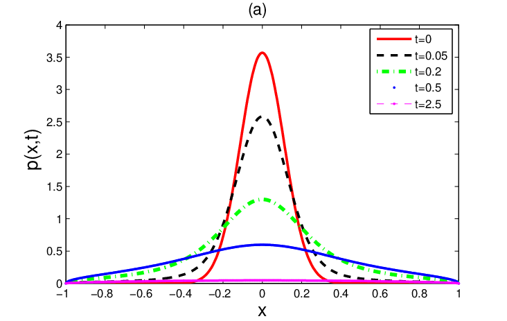
In this section, we investigate the probability density $p(x,t)$ that a ”particle” $X_{t}$ is located at the position $x$ at time $t$ given the probability profile of its initial position is Gaussian ( $\displaystyle p(x,0)=\sqrt{\frac{40}{\pi}}e^{-\frac{x^{2}}{40}}$ ) or uniform ( $\displaystyle p(x,0)=\dfrac{1}{2}I_{\{|x|<1\}}$ ). The absorbing condition implies the ”particle” will vanish once it is out of a specified domain. Figure 5 shows a time sequence of the probability densities for the symmetric $\alpha$ -stable Lévy process without any deterministic driving force $f=0$ or any Gaussian diffusion $d=0$ but with $\alpha=1$ and $\varepsilon=1$ at times $t=0,0.05,0.2,0.5,2.5$ . As shown in Fig. 5(a), for an initial Gaussian distribution, the density profiles keep the bell-type shape for small times while the probabilities near the center decreases faster than those away further from the center. For an initial uniform distribution, Fig. 5(b) demonstrates the density profile becomes a smooth function after $t>0$ , indicating the $\alpha$ -stable process has the effect of ”diffusion”. In this case, the maximum of the density function stays at the center of the domain, because the center is the furthest away from the boundary of the domain. In all cases, the ”particle” eventually escapes the bounded domain and vanishes afterwards.

5.2.1 Effect of different jump measures

Next, we examine the dependence of the probability density $p$ on the values of $\alpha$ (different Lévy measures) for symmetric $\alpha$ -stable Lévy motion ( $d=0$ and $f\equiv 0$ ). Figure 6 shows the density $p$ as a function of the position $x$ for $\alpha=0.1,0.5,1,1.5,1.9,2$ at two different times $t=0.25$ and $t=2.5$ , starting from the same Gaussian distribution $\displaystyle p(x,0)=\sqrt{\frac{40}{\pi}}e^{-\frac{x^{2}}{40}}$ .

If the particle starts near the center of the domain (the origin $x=0$ in our configuration), the numerical results in Fig. 6 show that, for $x$ near the origin, the probability $p$ is smaller as the value of $\alpha$ increases, suggesting that the particle is less likely to stay near the origin when the value $\alpha$ is larger. At earlier times, for example $t=0.25$ , the probability of finding the particle at positions $x$ away from the origin is larger when $\alpha$ is larger (except for the special Gaussian noise case $\alpha=2$ ). Note that the probability density for the Gaussian diffusion ( $\alpha=2$ ) is much smaller than those for the symmetric $\alpha$ -stable Lévy motion with $\alpha<2$ . The profiles of the density function change to parabola-like shape, having negative second-order derivative, for large values of $\alpha$ ( $\alpha\geq 1.5$ at time $t=0.25$ in our case), while the profiles stay bell-type shape for smaller values of $\alpha$ . At later times, for example $t=2.5$ , the probability near the boundary of the domain becomes a decreasing function of $\alpha$ for the values of $0.5\leq\alpha\leq 2$ , and the profiles of the density functions become all parabola-like except for the smallest value of $\alpha=0.1$ . It is interesting to point out that the probability $p$ appears to be discontinuous at the boundary $x=\pm 1$ for $\alpha=0.1$ and $0.5$ . Examining the solutions more closely near the boundaries, we find that the probability densities are actually continuous but have very sharp transition (a thin ”boundary layer”) at the boundaries. However, in our earlier work [11], the numerical results show that the mean first exit time of symmetric $\alpha$ -stable Lévy motion is discontinuous at the boundary of a bounded domain for $\alpha<1$ .

On the other hand, when the initial condition is uniformly distributed (i.e., the particle is equally likely starting from any point in the interval $[-1,1]$ ), the results in Fig. 7 show that the probability of finding the ”particle” near the center of the domain is a non-monotone function of $\alpha$ , while the probability near the boundary of the domain is a decreasing function of $\alpha$ for all values of $\alpha$ in $(0,2]$ . The profiles of the probability function changes from the starting shape of a step function to that of parabola-like for $\alpha\geq 1$ . In contrast, for small values of $\alpha$ (such as $\alpha=0.1$ ), the probability function keeps its flat profile as time elapses. Again, the functions are continuous at the boundary $x=\pm 1$ after a careful examination of the solutions near the boundary.

Next, we investigate the effect of the magnitude of Lévy noises. Figure 8 shows the probability density function $p$ at time $t=1$ starting from the initial profile $\displaystyle p(x,0)=\sqrt{\frac{40}{\pi}}e^{-\frac{x^{2}}{40}}$ for the case of pure non-Gaussian noise $d=0$ , $\alpha=1$ , the domain $D=(-1,1)$ and no deterministic driving force $f\equiv 0$ but different magnitude of $\varepsilon=0,0.1,0.5,1$ . When the noise is absent $\varepsilon=0$ , the probability density keep the initial profile $p(x,t)=p(x,0)$ . As the amount of noise $\varepsilon$ increases, the density function becomes smaller at the center of the domain and the function profile becomes flatter. Comparing with Figs. 5(a) and 6(a), we find that increasing the magnitude of Lévy noises has the similar effect as increasing the time or the value of $\alpha$ .

5.2.2 Effect of the deterministic driving force due to Ornstein-Uhlenbeck(O-U) potential: $f(x)=-x$

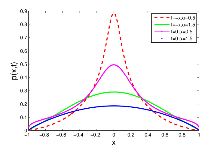
Next, we examine the effect of a deterministic driving force, the O-U potential $f(x)=-x$ , on the probability density function $p$ . The initial condition is the Gaussian profile $\displaystyle p(x,0)=\sqrt{\frac{40}{\pi}}e^{-\frac{x^{2}}{40}}$ as in Fig. 6. We keep other parameters the same as those in Fig. 6: $d=0$ and $\varepsilon=1$ . The O-U potential drives the ”particle” toward the origin ( $x=0$ ), the center of the domain, while the stochastic term in the SDE (1) acts like a ”diffusional” force. Figure 9 gives us the result of the competition between the two forces. At the smaller value of $\alpha=0.5$ , we compare the density functions $p$ at time $t=1$ with the driving force $f(x)=-x$ and without any deterministic force $f\equiv 0$ . As expected, we find that the probability of finding the particle near the origin or the boundary is higher or lower respectively when the O-U potential is present. At the larger value of $\alpha=1.5$ , the probability near the center is higher when the O-U potential is present, while the probabilities are almost identical near the boundary whether $f(x)=-x$ or $f=0$ .

As expected, adding the Gaussian noise $d\neq 0$ would decrease the probability density function. Figure 10 shows the density functions $p$ at time $t=1$ with the O-U potential $f(x)=-x$ and $\varepsilon=1,\alpha=0.5,1.5$ for different amount of Gaussian noises $d=0,0.1,0.5,1$ . For the smaller value of $\alpha=0.5$ , shown in Fig. 10(a), the density function profiles change from a bell-like shape to a parabola-like one as the Gaussian noise $d$ increases. However, for the larger value $\alpha=1.5$ , the density profiles at $t=1$ are parabola-like regardless the value of $d$ . As we have observed earlier, the Lévy noise with larger values of $\alpha$ has similar diffusive effect as the Gaussian noise on the probability density function.

5.2.3 Dependence on the size of the domain

In Fig. 11, we plot the probability densities at $t=1$ for three different sizes of domains $(-1,1)$ , $(-2,2)$ and $(-4,4)$ and three different values of $\alpha=0.5,1$ and $1.5$ . Here, the O-U potential $f(x)=-x$ is present but there is no Gaussian noise $d=0$ , and the initial profile of the probability density is the same Gaussian one as before. At a fixed value $x$ , the density function has higher value as the domain size increases due to the fact that it is harder to escape a larger domain. For the smaller value of $\alpha=0.5$ , Fig. 11(a) shows that the density function values are relatively insensitive to the domain sizes in the regions near the center, the region $(-0.5,0.5)$ in this case. It suggests that, for small values of $\alpha$ , the ”particle” escape the bounded domains mostly via large jumps rather than small movement. For the two other values of $\alpha=1$ and $1.5$ , the density function is smaller for the smaller domain $D=(-1,1)$ , but the probability functions have similar values near the center for the two larger domains $(-2,2)$ and $(-4,4)$ . The results shown in Fig. 11 imply that, for each value of $\alpha$ , there is a threshold for the size of the domain beyond which the density functions will have similar values in the regions centered at the origin.

5.3 Natural condition

The distribution and the properties of $\alpha-$ stable random variables are well known. However, the time evolution of the probability density of symmetric $\alpha-$ stable Lévy process is less well studied. We approximate the solution to the Fokker-Planck equation (4) subject to the natural far-field condition (6) by using the scheme (11) with increasing domain sizes until the PDF $p$ converges on the intervals of our interests.

To evaluate the error caused by replacing the infinity domain $(-\infty,\infty)$ for the natural condition with finite domains, we compute the integral $\displaystyle I_{p}(t)\equiv\int_{-\infty}^{\infty}p(x,t){\rm d}x$ . For the natural far-field condition, the integral $I_{p}(t)$ keeps its initial value of one for all times. For the case of $f\equiv 0,d=0$ , $\varepsilon=1$ , $\alpha=1$ , we compute the integral $I_{p}(1)$ numerically using trapezoidal rule based on the numerical solutions with increasing domain sizes $(a,b)=(-5,5),(-10,10),(-20,20)$ , $(-40,40)$ , $(-80,80)$ . The corresponding values of the integral for the different domain sizes are $0.997060069$ , $0.999318$ , $0.999838$ , $0.999961$ , $0.999990$ respectively. It is obvious that the integrals for these large domains are close to one, implying that the truncating the original infinite domain cause small amount of error. The integral is closer to one as the domain size becomes larger. The convergence order of the integral with respect to the domain size is about $2$ .

Starting with the same initial Gaussian profile $p(x,0)=\sqrt{\frac{40}{\pi}}e^{-\frac{x^{2}}{40}}$ , $d=0$ , $f(x)=-x$ , $\varepsilon=1$ and $\alpha=1.5$ , Fig. 12(a) shows the PDF $p$ on the interval $(-10,10)$ at time $t=1$ using increasing computational domain sizes $(-L,L)=(-10,10),(-20,20)$ , $(-30,30)$ , $(-40,40)$ . Note that the integro-differential equation (4) for the natural condition is different than Eq. (8) for the absorbing condition. Consequently, the corresponding numerical schemes are also different: (11) for the natural far-field condition and (9) for the absorbing condition. The numerical results show that the four different approximations fall onto each other, indicating that the probability $p$ becomes independent of domain size when the domain is large enough. In Fig. 12(b), we demonstrate the convergence of the value of the probability $p$ at the point $(x,t)=(9,1)$ . In this case, the values of $p$ on the interval $(-10,10)$ do not change significantly when the computational domain $(-L,L)$ includes $(-20,20)$ . Consequently, on the finite interval $(-10,10)$ , we can argue that the profile of $p$ obtained by using the computational domain larger than $(-20,20)$ shall agree well with that for natural far-field condition $(-\infty,\infty)$ . Comparing Fig. 12(a) with Fig. 11(c), we point out that the values of the density function for the natural condition near the center are slightly larger than those for the absorbing condition, when the other conditions match with each other.

Figure 12(c) and (d) show the PDF for $\alpha=0.5$ , keeping the other conditions the same. Again, the numerical solution converges for large enough computational domain. However, with other conditions being identical, the values of the PDF for natural condition near the center, shown in Fig.12(c), are significantly higher than those for the absorbing condition shown in Fig. 11(a).

The conclusions from comparing the two auxiliary conditions are the same when we remove the deterministic driving force $f$ . Figure 13 shows the PDFs for both auxiliary conditions on the same graph.

5.3.1 Deterministic force driven by the double-well potential: $f(x)=x-x^{3}$

The deterministic force governed by the double-well potential, $f(x)=x-x^{3}$ , drives the ’particle’ toward the two stable states $x=\pm 1$ . The potential has a local maximum located at the center $x=0$ and two local minima symmetrically located at $x=\pm 1$ . In the absence of noises, the ’particle’ would be driven to one of the stable steady states $x=\pm 1$ and stays there. Under the natural condition, we compute the probability density starting with a Gaussian profile centered at one of the stable state $x=-1$ , as shown in Fig. 14. From the numerical results, we observe that, although there is no particle concentrated around the stable position $x=1$ at the beginning, as time goes by, the probability density functions show two peaks centered at the two stable points $x=\pm 1$ respectively. It suggests the particles tend to stay at one of two stable points $x=\pm 1$ with nearly equal chance. At the same time, the peaks for $\alpha=0.5$ are more pronounced than those for $\alpha=1.5$ . On the other hand, the peak at $x=1$ for $\alpha=1.5$ approaches the same height as the original peak at $x=-1$ faster than the case of $\alpha=0.5$ .

6 Conclusion

The Fokker-Planck equation for a stochastic system with Brownian motion (a Gaussian process) is a local differential equations, while that for a stochastic system with a $\alpha-$ stable Lévy motion (a non-Gaussian process) is a nonlocal differential equation.

By exploring the Toeplitz matrix structure of the discretization, we have developed a fast and accurate numerical algorithm to solve the nonlocal Fokker-Planck equations, under either absorbing or natural conditions. We have found the conditions under which the schemes satisfy a maximum principle, and consequently, have shown their stability and the convergence based on the maximum principle.

The algorithm is tested and validated by comparing with an exact solution and well-known numerical solutions for the probability density functions of $\alpha$ -stable random variables. It is applied to two stochastic dynamical systems (i.e., the Ornstein-Uhlenbeck system and double-well system) with non-Gaussian Lévy noises. We find that the $\alpha$ -stable process has smoothing effect just as the standard diffusion: an initially non-smooth probability density function instantly becomes smooth for time $t>0$ . The value of $\alpha$ has significant effect on the profiles of the density functions.

Acknowledgments

We would like to thank Zhen-Qing Chen, Cyril Imbert, Renming Song and Jiang-Lun Wu for helpful discussions. This work was partly supported by the NSF Grants 0923111 and 1025422, and the NSFC grants 10971225 and 11028102.

References

[1] S. Albeverrio, B. Rüdiger, and J. L. Wu, Invariant measures and symmetry property of Lévy type operators, Potential Analysis, 13 (2000), pp. 147–168.
[2] , Analytic and probabilistic aspects of Lévy processes and fields in quantum theory, in Lévy Processes: Theory and Applications, O. E. Barndorff-Nielsen, T. Mikosch, and S. I. Resnick, eds., Boston, 2001, Birkhauser, pp. 187–224.
[3] D. Applebaum, Lévy Processes and Stochastic Calculus, Cambridge University Press, 2nd Edition, 2009.
[4] Harald Bergström, On some expansions of stable distribution functions, Arkiv för Matematik, 2 (1952), pp. 375–378.
[5] Alfonso Bueno-Orovio, David Kay, and Kevin Burrage, Fourier spectral methods for fractional-in-space reaction-diffusion equations, OCCAM, (2012).
[6] John M Chambers, Colin L Mallows, and BW Stuck, A method for simulating stable random variables, Journal of the American Statistical Association, 71 (1976), pp. 340–344.
[7] Z. Chen, P. Kim, and R. Song, Heat kernel estimates for Dirichlet fractional Laplacian, J. European Math. Soc., 12 (2010), pp. 1307–1329.
[8] Q. Du, M. Gunzburger, RB Lehoucq, and K. Zhou, Analysis and approximation of nonlocal diffusion problems with volume constraints, SIAM Review, 54 (2012), p. 627.
[9] Qiang Du, Zhan Huang, and RB Lehoucq, Nonlocal convection-diffusion volume-constrained problems and jump processes, Sandia National Laboratories, Technical report, SAND 2013-5008J (2013).
[10] Vincent J Ervin, Norbert Heuer, and John Paul Roop, Numerical approximation of a time dependent, nonlinear, space-fractional diffusion equation, SIAM Journal on Numerical Analysis, 45 (2007), pp. 572–591.
[11] T. Gao, J. Duan, X. Li, and R. Song, Mean exit time and escape probability for dynamical systems driven by Lévy noise, SIAM J. Sci. Comput., To appear (2013).
[12] C. W. Gardiner, Handbook of Stochastic Methods, Springer, 3rd Ed., 2004.
[13] , Stochastic Methods, Springer, 4th Ed., 2009.
[14] Gene H Golub and Charles F Van Loan, Matrix computations, JHU Press, 4th Ed., 2012.
[15] Cyril Imbert, A non-local regularization of first order Hamilton–Jacobi equations, Journal of Differential Equations, 211 (2005), pp. 218–246.
[16] G.S. Jiang and D. Peng, Weighted eno schemes for Hamilton-Jacobi equations, SIAM Journal on Scientific computing, 21 (2000), pp. 2126–2143.
[17] GUANG-SHAN JIANG and CHI-WANG SHU, Efficient implementation of weighted ENO schemes, JOURNAL OF COMPUTATIONAL PHYSICS, 126 (1996), pp. 202–228.
[18] Can Li, Weihua Deng, and Yujiang Wu, Finite difference approximations and dynamics simulations for the Lévy fractional Klein-Kramers equation, Numerical Methods for Partial Differential Equations, 28 (2012), pp. 1944–1965.
[19] Mark M Meerschaert and Charles Tadjeran, Finite difference approximations for fractional advection–dispersion flow equations, Journal of Computational and Applied Mathematics, 172 (2004), pp. 65–77.
[20] John P Nolan, Numerical calculation of stable densities and distribution functions, Communications in statistics. Stochastic models, 13 (1997), pp. 759–774.
[21] K. Sato, Lévy Processes and infinitely divisible distributions, Cambridge University Press, Cambridge, U.K., 1999.
[22] D. Schertzer, M. Larcheveque, J. Duan, V. Yanovsky, and S. Lovejoy, Fractional Fokker–Planck equation for nonlinear stochastic differential equations driven by non-gaussian Lévy stable noises, J. Math. Phys., 42 (2001), pp. 200–212.
[23] Chi-Wang Shu and Stanley Osher, Efficient implementation of essentially non-oscillatory shock-capturing schemes, Journal of Computational Physics, 77 (1988), pp. 439–471.
[24] A. Sidi and M. Israeli, Quadrature methods for periodic singular and weakly singular Fredholm integral equations, J. Sci. Comput., 3 (1988), pp. 201–231.
[25] W. A. Woyczynski, Lévy processes in the physical sciences, in Lévy Processes: Theory and Applications, O. E. Barndorff-Nielsen, T. Mikosch, and S. I. Resnick, eds., Boston, 2001, Birkhauser, pp. 241–266.
[26] Qianqian Yang, Fawang Liu, and I Turner, Numerical methods for fractional partial differential equations with Riesz space fractional derivatives, Applied Mathematical Modelling, 34 (2010), pp. 200–218.

Fokker-Planck Equations for Stochastic Dynamical Systems with Symmetric Lévy Motions

Abstract

keywords

AMS

1 Introduction

2 Fokker-Planck equations for SDEs with Lévy motions

2.1 Auxiliary Conditions

3 Numerical Methods

Remark 1.

4 Analysis of our numerical scheme

4.1 Discrete Maximum Principle

Proposition 1.

Proof.

Proposition 2.

Proof.

Proposition 3.

Proof.

Remark 2.

4.2 Stability and Convergence

Proposition 4.

Proof.

Remark 3.

5 Numerical results

5.1 Verification

5.2 Absorbing condition

5.2.1 Effect of different jump measures

5.2.2 Effect of the deterministic driving force due to Ornstein-Uhlenbeck(O-U) potential: f⁡(x)=−xf(x)=-x

5.2.3 Dependence on the size of the domain

5.3 Natural condition

5.3.1 Deterministic force driven by the double-well potential: f⁡(x)=x−x3f(x)=x-x^{3}

6 Conclusion

Acknowledgments

References

5.2.2 Effect of the deterministic driving force due to Ornstein-Uhlenbeck(O-U) potential: $f(x)=-x$

5.3.1 Deterministic force driven by the double-well potential: $f(x)=x-x^{3}$