跳到论文正文
W Papers独立论文阅读器 arXiv:1310.7611 论文正文 计算阅读时间 · 0%
引用这篇论文根据当前论文元数据生成,正式投稿前建议核对。


License: arXiv.org perpetual non-exclusive license
arXiv:1310.7611v1 [math.NA] 28 Oct 2013

Generalized time integration schemes for space-time moving finite elements

Randolph E. Bank ††thanks: Department of Mathematics, University of California, San Diego, La Jolla, California 92093-0112. Email: rbank@ucsd.edu. The work of this author was supported by the National Science Foundation under contract DMS-xxxxxxx.    Maximilian S. Metti ††thanks: Department of Mathematics, University of California, San Diego, La Jolla, California 92093-0112. Email: mmetti@ucsd.edu. The work of this author was supported by the National Science Foundation under contract DMS-xxxxxxx.
Abstract

In this paper, we analyze and provide numerical illustrations for a moving finite element method applied to convection-dominated, time-dependent partial differential equations. We follow a method of lines approach and utilize an underlying tensor-product finite element space that permits the mesh to evolve continuously in time and undergo discontinuous reconfigurations at discrete time steps. We employ the TR-BDF2 method as the time integrator for piecewise quadratic tensor-product spaces, and provide an almost symmetric error estimate for the procedure. Our numerical results validate the efficacy of these moving finite elements.

keywords
TR-BDF2, Moving Finite Elements, Arbitrary Lagrange-Eulerian Methods, Method of Characteristics, Convection-Dominated, Error Analysis
AMS
65M55, 65F10

1 Introduction

For parabolic equations, the method of lines is an efficient approach for computing a numerical solution by converting the partial differential equation into a coupled system of ordinary differential equations. This provides a great deal of flexibility in how the solution may be computed, as the time discretization then becomes independent of the spatial discretization. For finite element methods, the spatial dimensions are discretized in the usual way, leading to a semi-discrete problem that is subsequently propagated in time by numerical integration.

When dealing with convection-dominated problems, the spatial discretization can be chosen to evolve continuously in time, which allows the finite element mesh to continuously track moving structures in the solution such as steep sweeping fronts [baines1994moving, CARLSONMILLER1, CARLSONMILLER2]. These moving finite elements can lead to remarkably improved stability in computing a solution, with respect to the length of permissible time steps [MILLER1, MILLER2].

In [BANKMETTI, BANKSANTOS], tensor-product finite element spaces compatible with a method of lines discretization were introduced that allowed these moving finite element solutions to be studied in a space-time finite element framework. As a result, these papers established symmetric error estimates for these finite element solutions when the numerical time integrator belongs to a particular class of collocation methods. The first such symmetric error estimate is proven in [DUPONT82] for semi-discrete moving finite elements by using a mesh-dependent energy semi-norm, |||⋅||||\!|\!|\cdot|\!|\!|. To elaborate, a symmetric error estimate states that the finite element solution, uhu_{h}, satisfies

(1) ‖|u−uh|‖≤C​infχ∈𝒱h‖|u−χ|‖,|\!|\!|u-u_{h}|\!|\!|\leq C\inf_{\chi\in\mathcal{V}_{h}}|\!|\!|u-\chi|\!|\!|,

where uu is the true solution to the differential equation and 𝒱h\mathcal{V}_{h} is the (tensor-product) moving finite element space.

In this paper, we consider the effects of employing a time integrator that does not belong to the previous class of collocation methods. This is a valuable modification because collocation methods implicitly couple all intermediate stages of each time step, significantly increasing the computational complexity when using higher order quadrature. We consider the second-order and diagonally-implicit time integrator TR-BDF2 [A30, A30a], and using piecewise quadratic tensor-product finite element spaces to discretize the problem. This time integration scheme is known for its favorable stability properties [STRANG, hosea1996analysis, ying2009composite]. Moving finite element discretizations often lead to stiff systems of ODEs [MILLER1, MILLER2], which is why a stable time integration scheme is required. In Section 3, we prove an error estimate like (1) with an additional term introduced by TR-BDF2.

This work largely builds on the analyses in [BANKMETTI, METTITHESIS], where parts of the preliminary analysis are given in more detail. This paper is organized as follows: in Section 2, we describe the model equation, the piecewise quadratic tensor-product finite element space, and some preliminary results. In Section 3, a space-time moving finite element method using TR-BDF2 time integration is proposed and an error estimate for the finite element solution is proven. Section 4 describes and reports some numerical experiments that validate the efficacy of these moving finite element methods.

2 Preliminary Results

The model problem used in this error analysis is the linear convection-diffusion equation. The spatial domain, Ω\Omega, is assumed to be a simply connected set in ℝd\mathbb{R}^{d}, where d=1,2,d=1,2, or 33, with boundary ∂Ω\partial\Omega. The time domain is a finite interval, (0,T](0,T], and the space-time domain is given by ℱ≡Ω×(0,T]\mathcal{F}\equiv\Omega\times(0,T].

Let aa, bb, cc, and ff be smooth and bounded functions defined on ℱ\mathcal{F} such that there exist constants a¯>0\bar{a}>0 and c¯≥0\bar{c}\geq 0 with a≥a¯a\geq\bar{a} and c≥c¯c\geq\bar{c} on Ω\Omega, and let gg be piecewise continuous on ∂Ω\partial\Omega. Let u0u_{0} be a given initial condition for the solution on ℱ\mathcal{F} and let nn denote the outward unit normal vector to the boundary ∂Ω\partial\Omega. The solution to the differential equation, denoted by uu, is the function that satisfies

(2) ut−∇⋅(a∇u)+b⋅∇u+cu\displaystyle u_{t}-\nabla\cdot(a\nabla u)+b\cdot\nabla u+cu =f,\displaystyle=f, in​ℱ,\displaystyle\mathrm{in}\ \mathcal{F},
(3) a∇u⋅n\displaystyle a\nabla u\cdot n =g,\displaystyle=g, on​∂Ω×(0,T],\displaystyle\mathrm{on}\ \partial\Omega\times(0,T],
u⁡(x,0)\displaystyle u(x,0) =u0​(x),\displaystyle=u_{0}(x), for​x​in​Ω.\displaystyle\mathrm{for}\ x\ \mathrm{in}\ \Omega.

When the convection term, bb in (2), is large relative to the other coefficients, steep shock layers may develop in the solution that propagate through the spatial domain. Basic finite element discretizations consequently require short time steps to maintain accuracy of the computed solution at this moving front, or a moving mesh can be employed, allowing for more flexibility in the length of the time step. Moving finite elements offset the convection velocity in a similar manner to the method of characteristics. We assume a time dependent parametrization of the spatial domain, x⁡(t)x(t), and define the space-time derivative as

uτ​(x⁡(t),t)≡dd​t​u​(x⁡(t),t)=ut​(x⁡(t),t)+xt⋅∇u​(x⁡(t),t).u_{\tau}(x(t),t)\equiv\frac{d}{dt}u(x(t),t)=u_{t}(x(t),t)+x_{t}\cdot\nabla u(x(t),t).

We refer to this as the characteristic derivative of uu.

The weak form of the problem is: find uu with u​(t)∈ℋ1​(Ω)u(t)\in\mathcal{H}^{1}(\Omega) and ut​(t)∈ℒ2​(Ω)u_{t}(t)\in\mathcal{L}_{2}(\Omega) such that for all χ\chi in ℋ1​(Ω)\mathcal{H}^{1}(\Omega) and 0<t≤T0<t\leq T,

(4) (uτ​(⋅,t),χ)+𝒜τ​(t,u,χ)\displaystyle\big(u_{\tau}(\cdot,t),\chi\big)+\mathcal{A}_{\tau}(t;u,\chi) =(f⁡(⋅,t),χ)+⟨g⁡(⋅,t),χ⟩,\displaystyle=\big(f(\cdot,t),\chi\big)+\big\langle g(\cdot,t),\chi\big\rangle,
and when t=0t=0
(u⁡(⋅,0),χ)\displaystyle\big(u(\cdot,0),\chi\big) =(u0,χ).\displaystyle=\big(u_{0},\chi\big).

The inner-products are given by

(f,χ)\displaystyle(f,\chi) =∫Ωf⁡(x)​χ​(x)​𝑑x,\displaystyle=\int_{\Omega}f(x)\chi(x)\ dx,
⟨g,χ⟩\displaystyle\langle g,\chi\rangle =∫∂Ωg⁡(s)​χ​(s)​𝑑s,\displaystyle=\int_{\partial\Omega}g(s)\chi(s)\ ds,

and define the time-dependent bilinear form

𝒜τ(t;u,χ)≡∫Ωa(x,t)∇u(x,t)⋅∇χ(x)+(b(x,t)−xt(t))⋅∇u(x,t)χ(x)+c⁡(x,t)​u​(x,t)​χ​(x)​d​x.\mathcal{A}_{\tau}(t;u,\chi)\equiv\int_{\Omega}a(x,t)\nabla u(x,t)\cdot\nabla\chi(x)+(b(x,t)-x_{t}(t))\cdot\nabla u(x,t)\ \chi(x)\\ +c(x,t)u(x,t)\chi(x)\ dx.

Notice that parameterizing the spatial variable so that xt≈bx_{t}\approx b leads to a formulation where the convection velocity is much less prominent, as it is “absorbed” into the characteristic derivative.

The finite element space we use to discretize the differential equation is a tensor-product of a discontinuous piecewise quadratic finite elements in time with continuous piecewise quadratic finite elements in space.

Let 0<t1<…<tm=T0<t_{1}<\ldots<t_{m}=T form a strict ordered partition of the time domain and define Δ​ti≡ti−ti−1\Delta t_{i}\equiv t_{i}-t_{i-1}. For 1≤i≤m1\leq i\leq m, let {xk​(t)}\{x_{k}(t)\} represent the vertices of a triangulation of the domain at time tt, where 0≤k≤Ni0\leq k\leq N_{i}, and we assume that |xk​(t)−xj​(t)|>Δ​x|x_{k}(t)-x_{j}(t)|>\Delta x throughout each time partition for some minimum mesh size Δ​x>0\Delta x>0 and j≠kj\neq k. The vertices of the mesh are permitted to move along quadratic trajectories throughout each time partition—that is, each node xk​(t)x_{k}(t) is a quadratic polynomial for ti−1<t≤tit_{i-1}<t\leq t_{i} in time—though discontinuous reconfigurations of the mesh are permitted at the beginning of each partition. These discontinuous changes in the mesh provide flexibility for periodically adding and removing degrees of freedom, as well as keeping the nodes in the mesh from colliding and tangling.

Fig. 1: An example space-time mesh partition of a single dimension in space. The filled circles represent the space-time “hat” basis nodes; hollow circles correspond to basis nodes with basis functions that are the product of a “bump” function with a “hat” or “bump” function.

The reference element for this finite element space is the Cartesian product of the unit interval (d=1d=1), triangle (d=2d=2), or tetrahedron (d=3d=3) for space with the unit interval reference element for the time domain. Let ee be an element in the mesh with vertices given by xk​(t)x_{k}(t) at time tt, where k=0,1,…,dk=0,1,\ldots,d and ti−1≤t≤tit_{i-1}\leq t\leq t_{i}. Then the (isoparametric) mapping from the reference element to ee is given by

t\displaystyle t =ti−1+t^​Δ​ti,\displaystyle=t_{i-1}+\hat{t}\Delta t_{i},
x⁡(t)\displaystyle x(t) =𝒥e​(t)​x^+x0​(t),\displaystyle=\mathcal{J}_{e}(t)\hat{x}+x_{0}(t),

for 0≤t^≤10\leq\hat{t}\leq 1 and x^\hat{x} in the spatial reference element, where x⁡(t)x(t) is affine in space and quadratic in time, as the node trajectories are restricted to follow quadratic paths throughout the time partition. Notice that the time variable is space invariant, but the spatial variable does in fact depend on tt. The d×dd\times d spatial Jacobian matrix, 𝒥e​(t)\mathcal{J}_{e}(t), determines the shape and size of the element e⁡(t)e(t). Since the determinant of the spatial Jacobian is proportional to the size of the element, we require |det𝒥e​(t)|>0|\det\mathcal{J}_{e}(t)|>0 for all tt to ensure a non-degenerate mesh.

Since we are using a tensor-product space-time discretization, the degrees of freedom of the finite element space are distributed in time slices. Namely, for fixed time tt, the degrees of freedom {xk​(t)}\{x_{k}(t)\} define a standard finite element space of continuous piecewise-quadratic polynomials on Ω\Omega, which we denote by 𝒱h​(t)\mathcal{V}_{h}(t). This is an important property that is directly used in formulating the discrete problem. We emphasize that the finite element functions are piecewise quadratic polynomials along the trajectories of the space nodes xk​(t)x_{k}(t) defined via the isoparametric mapping, rather than in the time direction as with standard tensor-product discretizations. This ensures that the characteristic derivative of a finite element function, ϕ\phi, is continuous within each time partition and satisfies ϕτ​(t)∈𝒱h​(t)\phi_{\tau}(t)\in\mathcal{V}_{h}(t). We denote the tensor-product finite element space on the space-time domain by 𝒱h\mathcal{V}_{h}. More detailed descriptions of these tensor product finite element spaces can be found in [BANKMETTI, METTITHESIS].

For the error analysis of our moving finite element method, it is convenient to define the finite element functions at the mesh discontinuity by an ℒ2\mathcal{L}_{2}-projection. For ϕ\phi in 𝒱h\mathcal{V}_{h}, we represent the limiting values of ϕ\phi near the discontinuities as ϕ⁡(ti+)≡limδ→0+ϕ⁡(t+δ)\phi(t_{i^{+}})\equiv\lim_{\delta\rightarrow 0^{+}}\phi(t+\delta) and ϕ⁡(ti−)≡limδ→0+ϕ⁡(t−δ).\phi(t_{i^{-}})\equiv\lim_{\delta\rightarrow 0^{+}}\phi(t-\delta). Thus, we require

(ϕ⁡(ti+),χ)=(ϕ⁡(ti−),χ)(\phi(t_{i^{+}}),\chi)=(\phi(t_{i^{-}}),\chi)

for all χ\chi in 𝒱h​(ti+)\mathcal{V}_{h}(t_{i^{+}}), i=1,…,mi=1,\ldots,m. To uniquely determine the finite element functions, we take ϕ⁡(ti)≡ϕ⁡(ti−)\phi(t_{i})\equiv\phi(t_{i^{-}}) at the discontinuities.

Multi-index notation is used to represent spatial derivatives, but time and characteristic derivatives will not follow this convention. The ℋk​(Ω)\mathcal{H}^{k}(\Omega) semi-norm and norm follow conventional notation and we write

|v|k=(∑|α|=k(Dα​v,Dα​v))1/2and‖v‖k=(∑|α|≤k(Dα​v,Dα​v))1/2.|v|_{k}=\left(\sum_{|\alpha|=k}(D_{\alpha}v,D_{\alpha}v)\right)^{1/2}\quad\mathrm{and}\quad|\!|v|\!|_{k}=\left(\sum_{|\alpha|\leq k}(D_{\alpha}v,D_{\alpha}v)\right)^{1/2}.

Following Dupont [DUPONT82], a mesh-dependent semi-norm is defined that allows us to prove our error estimate,

‖v‖(−1,𝒱hp​(t))=supχ∈𝒱hp​(t)χ≠0|(v,χ)|‖χ‖1.|\!|v|\!|_{(-1,\mathcal{V}_{h}^{p}(t))}=\sup_{\begin{subarray}{c}\chi\in\mathcal{V}_{h}^{p}(t)\\ \chi\neq 0\end{subarray}}\frac{\left|(v,\chi)\right|}{|\!|\chi|\!|_{1}}.

We also use the infinity norm, ‖v‖∞=maxx∈Ω⁡|v⁡(x)||\!|v|\!|_{\infty}=\max_{x\in\Omega}|v(x)|.

We now introduce a space-time shape regularity constraint for the moving finite elements, that controls the time evolution of the spatial elements and prevents degenerate elements. Fix ee to be an element in the time partition with ti−1≤t≤tit_{i-1}\leq t\leq t_{i}. Then, the Jacobian matrix at time tt can be represented as

(5) 𝒥e​(t)=(ℛe​(t)+Δ​ti​ℋe​(t))​𝒥e​(ti−1+),\mathcal{J}_{e}(t)=\big(\mathcal{R}_{e}(t)+\Delta t_{i}\mathcal{H}_{e}(t)\big)\mathcal{J}_{e}(t_{i-1^{+}}),

for some orthogonal rotation matrix, ℛe​(t)\mathcal{R}_{e}(t), and evolution matrix, ℋe​(t)\mathcal{H}_{e}(t). The matrix ℛe+Δ​ti​ℋe\mathcal{R}_{e}+\Delta t_{i}\mathcal{H}_{e} is constrained to have quadratic polynomial entries throughout the time partition. The matrix ℛe​(t)\mathcal{R}_{e}(t) describes the element rotation in time, and the evolution matrix describes the deformation of the shape of the element. Since the trajectories of the spatial nodes are restricted to quadratic polynomial paths, elements cannot rotate perfectly in time and more of a twisting action is observed; the evolution matrix necessarily reflects these deformations. If an element is merely translated in time, without rotation or changing shape, then the Jacobian matrix, 𝒥e​(t)\mathcal{J}_{e}(t), remains unchanged.

Let ρ⁡(⋅)\rho(\cdot) represent the spectral radius for d×dd\times d matrices. It is assumed that the evolution matrix ℋe\mathcal{H}_{e} has a uniformly bounded spectral radius throughout the time step; namely, there exists some positive constant μ\mu that does not depend on ee or tt such that

(6) ρ⁡(ℋe​(t))≤μ.\rho\big(\mathcal{H}_{e}(t)\big)\leq\mu.

This bounds the relative change in shape and size of the element over time. Assuming a non-degenerate finite element space and the space-time shape regularity bound (6), it follows that

(7) ρ⁡(𝒥e​(t)​𝒥e−1​(ti−1+))=ρ⁡(ℛe​(t)+Δ​ti​ℋe​(t))≤1+μ​Δ​ti\rho\big(\mathcal{J}_{e}(t)\mathcal{J}_{e}^{-1}(t_{i-1^{+}})\big)=\rho\big(\mathcal{R}_{e}(t)+\Delta t_{i}\mathcal{H}_{e}(t)\big)\leq 1+\mu\Delta t_{i}

and, for c~μ,d=[(1+μ​Δ​ti)d−1]/Δ​ti=𝒪⁡(1)\tilde{c}_{\mu,d}=[(1+\mu\Delta t_{i})^{d}-1]/\Delta t_{i}=\mathcal{O}(1) and Δ​ti≤1/2​c~μ,d\Delta t_{i}\leq 1/2\tilde{c}_{\mu,d},

(8) (1−c~μ,d​Δ​ti)≤(1−μ​Δ​ti)d≤𝒟e​(t)𝒟e​(ti−1+)=det(𝒥e​(t)​𝒥e−1​(ti−1+))≤(1+μ​Δ​ti)d≤(1+c~μ,d​Δ​ti),(1-\tilde{c}_{\mu,d}\Delta t_{i})\leq(1-\mu\Delta t_{i})^{d}\leq\frac{\mathcal{D}_{e}(t)}{\mathcal{D}_{e}(t_{i-1^{+}})}\\ =\det\big(\mathcal{J}_{e}(t)\mathcal{J}_{e}^{-1}(t_{i-1^{+}})\big)\leq(1+\mu\Delta t_{i})^{d}\leq(1+\tilde{c}_{\mu,d}\Delta t_{i}),

since ℛe\mathcal{R}_{e} is an orthogonal matrix.

Let ϕ\phi be a function in the finite element space 𝒱h​(t)\mathcal{V}_{h}(t) for some tt in the time partition (ti−1,ti](t_{i-1},t_{i}]. We shift ϕ\phi onto the mesh of 𝒱hp​(ti−1+)\mathcal{V}_{h}^{p}(t_{i-1^{+}}), at the beginning of the time partition by replacing the basis functions of 𝒱h​(t)\mathcal{V}_{h}(t) with with their corresponding basis functions in 𝒱h​(ti−1+)\mathcal{V}_{h}(t_{i-1^{+}}), while preserving the basis coefficients. Formally, this operation can be defined by an element-wise composition of the inverse of the affine spatial isoparametric maps for the elements in the mesh at time tt, which is well-defined for non-degenerate meshes, with the affine spatial isoparametric maps for the elements at the beginning of the time step ti−1+t_{i-1^{+}}. The following lemma, proven in [METTITHESIS], establishes the relationship between the space-time shape regularity constraint (6) and the continuity of this shift operation.

Lemma 1 (Shift Lemma).

Let ϕ,χ∈𝒱h​(t)\phi,\chi\in\mathcal{V}_{h}(t) and ϕ~,χ~∈𝒱h​(ti−1+)\tilde{\phi},\tilde{\chi}\in\mathcal{V}_{h}(t_{i-1^{+}}) represent a pair of finite element functions and their shifts, respectively, on a non-degenerate time partition of the mesh that satisfies (6) on each element. If Δ​ti≤1/2​c~μ,d\Delta t_{i}\leq 1/2\tilde{c}_{\mu,d}, as defined in (8), then there exists a positive constant Cμ,dC_{\mu,d} such that

(9) |(ϕ,χ)−(ϕ~,χ~)|\displaystyle\Big|\big(\phi,\chi\big)-\big(\tilde{\phi},\tilde{\chi}\big)\Big| ≤Cμ,d​Δ​ti​‖ϕ~‖02+‖χ~‖022,\displaystyle\leq C_{\mu,d}\Delta t_{i}\frac{\big|\!\big|\tilde{\phi}\big|\!\big|_{0}^{2}+\big|\!\big|\tilde{\chi}\big|\!\big|_{0}^{2}}{2},
(10) |‖ϕ‖02−‖ϕ~‖02|\displaystyle\Big|\big|\!\big|\phi\big|\!\big|_{0}^{2}-\big|\!\big|\tilde{\phi}\big|\!\big|_{0}^{2}\Big| ≤Cμ,d​Δ​ti​‖ϕ~‖02,\displaystyle\leq C_{\mu,d}\Delta t_{i}\big|\!\big|\tilde{\phi}\big|\!\big|_{0}^{2},
(11) |‖ϕ‖12−‖ϕ~‖12|\displaystyle\Big|\big|\!\big|\phi\big|\!\big|_{1}^{2}-\big|\!\big|\tilde{\phi}\big|\!\big|_{1}^{2}\Big| ≤Cμ,d​Δ​ti​‖ϕ~‖12.\displaystyle\leq C_{\mu,d}\Delta t_{i}\big|\!\big|\tilde{\phi}\big|\!\big|_{1}^{2}.

We now present a local Grönwall lemma that will be used to bound the maximum error of the finite element solution in the ℒ2\mathcal{L}_{2}-norm over each time partition. The original proof for this lemma is given in [METTITHESIS].

Lemma 2 (Local Grönwall Inequality).

Suppose there are two distinct times on each time partition, ti−1<ti,1<ti,2≤tit_{i-1}<t_{i,1}<t_{i,2}\leq t_{i}, when the mesh satisfies the regularity constraint (6) and that there exists a positive constant κ\kappa such that

(12) ‖b−xt‖∞≤κ.|\!|b-x_{t}|\!|_{\infty}\leq\kappa.

If Δ​ti≤1/2​c~μ,d\Delta t_{i}\leq 1/2\tilde{c}_{\mu,d}, as defined in (8), and functions ϕ\phi in 𝒱h\mathcal{V}_{h} and η\eta with η\eta in ℋ1​(Ω)\mathcal{H}^{1}(\Omega) and ητ\eta_{\tau} in ℒ2​(Ω)\mathcal{L}_{2}(\Omega) satisfy

(13) (ϕτ​(ti,j),χ)+𝒜τ​(ϕ⁡(ti,j),χ)=(ητ​(ti,j),χ)+𝒜τ​(η⁡(ti,j),χ)\big(\phi_{\tau}(t_{i,j}),\chi\big)+\mathcal{A}_{\tau}\big(\phi(t_{i,j}),\chi\big)=\big(\eta_{\tau}(t_{i,j}),\chi\big)+\mathcal{A}_{\tau}\big(\eta(t_{i,j}),\chi\big)

for all χ\chi in 𝒱h​(ti,j)\mathcal{V}_{h}(t_{i,j}) at time each collocation node j=1,2j=1,2, then, there exists a constant such that

max1≤j≤2⁡‖ϕ⁡(ti,j)‖02≤C⁡{‖ϕ⁡(ti−1+)‖02+∑j=12Δ​ti​(‖ητ​(ti,j)‖(−1,𝒱h​(ti,j))2+||η⁡(ti,j)||12+|​|ϕ⁡(ti,j)||12)},\max_{1\leq j\leq 2}\big|\!\big|\phi(t_{i,j})\big|\!\big|_{0}^{2}\\ \leq C\left\{\big|\!\big|\phi(t_{i-1^{+}})\big|\!\big|_{0}^{2}+\sum_{j=1}^{2}\Delta t_{i}\left(|\!|\eta_{\tau}(t_{i,j})|\!|_{(-1,\mathcal{V}_{h}(t_{i,j}))}^{2}+|\!|\eta(t_{i,j})|\!|_{1}^{2}+|\!|\phi(t_{i,j})|\!|_{1}^{2}\right)\right\},

where CC depends on κ,μ,d,p\kappa,\mu,d,p, and the differential equation.

Another discrete Grönwall lemma is used to aggregate the spatial error bounds from each time partition over the entire time domain. This result was proven in [SANTOSTHESIS].

Lemma 3 (Discrete Grönwall Inequality).

Let Δ​ti>0\Delta t_{i}>0 and αi,γi,θi,qi≥0\alpha_{i},\gamma_{i},\theta_{i},q_{i}\geq 0, for 1≤i≤m1\leq i\leq m, with θi​Δ​ti≤12\theta_{i}\Delta t_{i}\leq\frac{1}{2} and θ=maxi⁡θi\theta=\max_{i}\theta_{i}. Then, if

qi−qi−1Δ​ti+γi≤αi+θi​(qi+qi−1),\frac{q_{i}-q_{i-1}}{\Delta t_{i}}+\gamma_{i}\leq\alpha_{i}+\theta_{i}(q_{i}+q_{i-1}),

there exists a positive constant CθC_{\theta} such that

max1≤i≤m⁡qi+∑i=1mγi​Δ​ti≤Cθ​{q0+∑i=1mαi​Δ​ti}.\max_{1\leq i\leq m}q_{i}+\sum_{i=1}^{m}\gamma_{i}\Delta t_{i}\leq C_{\theta}\left\{q_{0}+\sum_{i=1}^{m}\alpha_{i}\Delta t_{i}\right\}.

3 A space-time moving finite element method with TR-BDF2

To achieve second-order accuracy for the finite element solution, we employ the two-stage, diagonally-implicit time integration scheme TR-BDF2. Since this scheme is diagonally implicit, significant time savings are realized when it is applied to large systems of ODEs, including systems arising from a method of lines discretization of a parabolic equation. TR-BDF2 was proposed by Bank, et al. in [A30, A30a] and has been analyzed in several other papers for its efficiency and stability [STRANG, hosea1996analysis, ying2009composite]. TR-BDF2 actually refers to a family of time stepping methods that is parametrized by the location of the intermediate basis node. For this method, we define the collocation nodes on the reference element to be

t^0=0,t^1=ε/2,andt^2=1,\hat{t}_{0}=0,\quad\hat{t}_{1}={\varepsilon}/{2},\quad\mathrm{and}\quad\hat{t}_{2}=1,

where 0<ε<10<\varepsilon<1 is a free parameter that determines the exact time stepping scheme within the TR-BDF2 family. We choose the reference element’s basis nodes to be

ζ^0=0,ζ^1=ε,andζ^2=1\hat{\zeta}_{0}=0,\quad\hat{\zeta}_{1}={\varepsilon},\quad\mathrm{and}\quad\hat{\zeta}_{2}=1

so that t^1\hat{t}_{1} is the midpoint of the first two basis nodes. The Runge-Kutta coefficients correspond to integrating the computed solution a step of length ε​Δ​ti\varepsilon\Delta t_{i} by the trapezoid rule, then completing the time step by a second-order backward Euler difference: let u⁡(t)u(t) denote an approximate solution of some system of ODEs, then the solution is computed using the approximations

uT​R​(ti,1)\displaystyle u_{TR}(t_{i,1}) =12​u​(ζi,1)+12​u​(ζi,0),\displaystyle=\frac{1}{2}u(\zeta_{i,1})+\frac{1}{2}u(\zeta_{i,0}),
u⁡(ti,2)\displaystyle u(t_{i,2}) =u⁡(ζi,2),\displaystyle=u(\zeta_{i,2}),

at the collocation nodes, where the isoparametric map is use to distribute the basis and collocation nodes throughout the time domain

ζi,j=ti−1+ζ^j​Δ​tiandti,k=ti−1+t^k​Δ​ti\zeta_{i,j}=t_{i-1}+\hat{\zeta}_{j}\Delta t_{i}\quad\mathrm{and}\quad t_{i,k}=t_{i-1}+\hat{t}_{k}\Delta t_{i}

for j=0,1,2j=0,1,2 and k=1,2k=1,2. The coefficients for the time derivative are determined by the interpolating quadratic Lagrange polynomials associated with the degrees of freedom in the time discretization evaluated at the collocation nodes:

δ¯t​u​(ti,1)\displaystyle\bar{\delta}_{t}u(t_{i,1}) =1ε​u​(ζi,1)−1ε​u​(ζi,0),\displaystyle=\frac{1}{\varepsilon}u(\zeta_{i,1})-\frac{1}{\varepsilon}u(\zeta_{i,0}),
δ¯t​u​(ti,2)\displaystyle\bar{\delta}_{t}u(t_{i,2}) =2−ε1−ε​u​(ζi,2)−1ε⁡(1−ε)​u​(ζi,1)+1−εε​u​(ζi,0).\displaystyle=\frac{2-\varepsilon}{1-\varepsilon}u(\zeta_{i,2})-\frac{1}{\varepsilon(1-\varepsilon)}u(\zeta_{i,1})+\frac{1-\varepsilon}{\varepsilon}u(\zeta_{i,0}).

The optimal choice for the parameter is known to be ε=2−2\varepsilon=2-\sqrt{2}, as it minimizes the local truncation error and we refer to the choice ε=2−2\varepsilon=2-\sqrt{2} as the Richardson basis node [choudhury1992waveform, ying2009composite]. The TR-BDF2 scheme is A-stable and L-stable [A30, A30a, hosea1996analysis]. These stability properties are important as method of lines discretizations of (4) typically lead to stiff systems of ODEs [MILLER1, MILLER2].

In this section, we use the TR-BDF2 method to integrate the semi-discrete system of ODEs given by the method of lines applied to a moving finite element discretization, as described in Section 2 of the weak form of the differential equation (4). Fix ii to index some time partition and let uh∈𝒱hu_{h}\in\mathcal{V}_{h}; let u~h​(t)\tilde{u}_{h}(t) represent the function shifted onto the mesh at the mid-step collocation node t=ti,1t=t_{i,1} and u^h​(t){\hat{u}}_{h}(t) represent the function shifted onto the mesh at the end-step collocation node t=ti,2t=t_{i,2}. The discrete problem can be characterized as finding the finite element function uh{u}_{h} that satisfies

(14) (u~h​(ζi,1)−u~h​(ζi,0)ε​Δ​ti,χ~)+𝒜τ​(u~h​(ζi,1)+u~h​(ζi,0)2,χ~)=(f⁡(ti,1),χ~)+⟨g⁡(ti,1),χ~⟩\Big(\frac{\tilde{u}_{h}(\zeta_{i,1})-\tilde{u}_{h}(\zeta_{i,0})}{\varepsilon\Delta t_{i}},\tilde{\chi}\Big)+\mathcal{A}_{\tau}\Big(\frac{\tilde{u}_{h}(\zeta_{i,1})+\tilde{u}_{h}(\zeta_{i,0})}{2},\tilde{\chi}\Big)=\big(f(t_{i,1}),\tilde{\chi}\big)+\big\langle g(t_{i,1}),\tilde{\chi}\big\rangle

for all χ~\tilde{\chi} in 𝒱h​(ti,1)\mathcal{V}_{h}(t_{i,1}) at each mid-step collocation node t=ti,1t=t_{i,1}, and for all χ^{\hat{\chi}} in 𝒱h​(ti,2)\mathcal{V}_{h}(t_{i,2}),

(15) (ε⁡(2−ε)​u^h​(ζi,2)−u^h​(ζi,1)+(1−ε)2​u^h​(ζi,0)ε⁡(1−ε)​Δ​ti,χ^)+𝒜τ​(u^h​(ζi,2),χ^)=(f⁡(ti,2),χ^)+⟨g⁡(ti,2),χ^⟩,\Big(\frac{\varepsilon(2-\varepsilon){\hat{u}}_{h}(\zeta_{i,2})-{\hat{u}}_{h}(\zeta_{i,1})+(1-\varepsilon)^{2}{\hat{u}}_{h}(\zeta_{i,0})}{\varepsilon(1-\varepsilon)\Delta t_{i}},{\hat{\chi}}\Big)+\mathcal{A}_{\tau}({\hat{u}}_{h}(\zeta_{i,2}),{\hat{\chi}})\\ =\big(f(t_{i,2}),{\hat{\chi}}\big)+\big\langle g(t_{i,2}),{\hat{\chi}}\big\rangle,

i=1,…,mi=1,\ldots,m. In contrast to the weak formulation (4), the discrete problem weakly enforces the differential equation only at the collocation nodes. The constraint

(16) (uh​(ti+),χ)=(uh​(ti−),χ)({u}_{h}(t_{i^{+}}),\chi)=({u}_{h}(t_{i^{-}}),\chi)

must also hold for all χ\chi in 𝒱h​(ti+)\mathcal{V}_{h}(t_{i^{+}}), i=1,…,mi=1,\ldots,m, to ensure that uh∈𝒱h{u}_{h}\in\mathcal{V}_{h}.

We now prove an error estimate for (14)–(16). Our proof follows that of Theorem 4.3 in [BANKMETTI] with some additional arguments that bound the error introduced by the trapezoid approximation at the mid-step of each time partition. Due to the departure of this method from a strict finite element framework, the symmetry of the error bound is broken and an additional term proportional to the error of the trapezoid approximation is introduced. We must also assume the bound ‖aτ‖∞≤α|\!|a_{{\tau}}|\!|_{\infty}\leq\alpha, for some α>0\alpha>0 on the characteristic derivative of the diffusion coefficient.

One final aspect in which the error bound changes is that the TR-BDF2 increases sensitivity to the discontinuous changes in the mesh at the beginning of the time steps, compared to the collocation methods used in [BANKMETTI]. Recently, Bank and Yserentant [BANKYSERENTANT] proved the ℋ1\mathcal{H}^{1}-stability of ℒ2\mathcal{L}_{2}-projections onto finite element spaces with potentially nonuniform meshes. Using this result, we assume |χ⁡(ti+)|1≤Cℋ​|χ⁡(ti−)|1|\chi(t_{i^{+}})|_{1}\leq C_{\mathcal{H}}|\chi(t_{i^{-}})|_{1}, for χ\chi in 𝒱h\mathcal{V}_{h}. As can be seen from [BANKYSERENTANT], the bounding constant, CℋC_{\mathcal{H}}, is smaller when the mesh reconfiguration is more subtle at the mesh discontinuities. This intuitively makes sense, since χ⁡(ti+)≈χ⁡(ti−)\chi(t_{i^{+}})\approx\chi(t_{i^{-}}) in such cases. For a given differential equation, since 0<a¯≤a≤‖a‖∞0<\bar{a}\leq a\leq|\!|a|\!|_{\infty}, we have an equivalence of norms

1c𝒜||a1/2(ti)∇ϕ||0≤|ϕ|1≤c𝒜||a1/2(ti)∇ϕ||0\frac{1}{c_{\mathcal{A}}}|\!|a^{1/2}(t_{i})\nabla\phi|\!|_{0}\leq|\phi|_{1}\leq c_{\mathcal{A}}|\!|a^{1/2}(t_{i})\nabla\phi|\!|_{0}

for some positive c𝒜c_{\mathcal{A}}. We define the stability constant for the diffusion-weighted semi-norm by

(17) |a1/2(ti)∇ϕ(ti+)|02≤C𝒜,ℋ|a1/2(ti)∇ϕ(ti−)|02.|a^{1/2}(t_{i})\nabla\phi(t_{i^{+}})|_{0}^{2}\leq C_{\mathcal{A},\mathcal{H}}|a^{1/2}(t_{i})\nabla\phi(t_{i^{-}})|_{0}^{2}.

The norm in which the error is bounded employs the trapezoid approximation at the mid-step collocation node of each time partition. Let uu be some function defined on ℱ\mathcal{F} and uT​R​(ti,1)≡(u~​(ζi,1)+u~​(ζi,0))/2∈𝒱h​(t)u_{TR}(t_{i,1})\equiv(\tilde{u}(\zeta_{i,1})+\tilde{u}(\zeta_{i,0}))/{2}\in\mathcal{V}_{h}(t), where u~​(t)\tilde{u}(t) represents uu evaluated at time tt following the characteristic from time ti,1t_{i,1} (meaning u~​(t)\tilde{u}(t) represents the function uu shifted onto the mesh at time ti,1t_{i,1}.) The semi-norm in which we bound the error of the finite element solution with TR-BDF2 time integration is

‖|u|‖2≡max1≤i≤m1≤j≤2⁡‖u⁡(ti,j)‖02+∑i=1mΔ​ti​(||δ¯τ​u​(ti,1)||(−1,𝒱h​(ti,1))2+|​|uT​R​(ti,1)||12CLOSEOPEN+‖u⁡(ζi,1)‖12+||δ¯τ​u​(ti−)||(−1,𝒱h​(ti−))2+|​|u⁡(ti−)||12).|\!|\!|u|\!|\!|^{2}\equiv\max_{\begin{subarray}{c}1\leq i\leq m\\ 1\leq j\leq 2\end{subarray}}|\!|u(t_{i,j})|\!|_{0}^{2}+\sum_{i=1}^{m}\Delta t_{i}\big(|\!|\bar{\delta}_{{\tau}}u(t_{i,1})|\!|_{(-1,\mathcal{V}_{h}(t_{i,1}))}^{2}+|\!|u_{TR}(t_{i,1})|\!|_{1}^{2}\\ +|\!|u(\zeta_{i,1})|\!|_{1}^{2}+|\!|\bar{\delta}_{{\tau}}u(t_{i^{-}})|\!|_{(-1,\mathcal{V}_{h}(t_{i^{-}}))}^{2}+|\!|u(t_{i^{-}})|\!|_{1}^{2}\big).
Theorem 4.

Suppose that 𝒱h\mathcal{V}_{h} is a finite element space with a non-degenerate mesh and let ε=2/3\varepsilon=2/3. Furthermore, assume that there exist positive constants α\alpha, μ\mu, and κ\kappa such that at each collocation node

(18) ‖aτ‖∞\displaystyle|\!|a_{\tau}|\!|_{\infty} ≤α,\displaystyle\leq\alpha,
(19) ρ⁡(ℋe)\displaystyle\rho\big(\mathcal{H}_{e}\big) ≤μ,\displaystyle\leq\mu,
(20) ‖b−xt‖∞\displaystyle|\!|b-x_{t}|\!|_{\infty} ≤κ,\displaystyle\leq\kappa,

and that the mesh discontinuities are controlled and the spatial meshes and length of the time steps are graded so that

(21) C𝒜,ℋ\displaystyle C_{\mathcal{A},\mathcal{H}} ≤7/2\displaystyle\leq{7}/{2}
and
(22) Δ​ti\displaystyle\Delta t_{i} ≤2​Δ​ti−1.\displaystyle\leq 2\Delta t_{i-1}.

Then, if Δ​t=max1≤i≤m⁡Δ​ti\Delta t=\max_{1\leq i\leq m}\Delta t_{i} is sufficiently small, there exists a positive constant CC such that the finite element solution satisfies

(23) ‖|u−u¯|‖2≤C⁡{infχ∈𝒱h‖|u−χ|‖2+∫0T‖Δ​ti2​uτ​τ​(t)‖12​𝑑t},|\!|\!|u-\bar{u}|\!|\!|^{2}\leq C\Big\{\inf_{\chi\in\mathcal{V}_{h}}|\!|\!|u-\chi|\!|\!|^{2}+\int_{0}^{T}|\!|\Delta t_{i}^{2}u_{\tau\tau}(t)|\!|_{1}^{2}\ dt\Big\},

where CC depends on μ,κ,d,p\mu,\kappa,d,p, and the differential equation.

Note that this proof is restricted to the case where we use the collocation nodes determined by Gauss-Radau quadrature, ε=2/3\varepsilon=2/3, as Gauss-Radau quadrature has a positive truncation error, which helps bound the aggregation of the local truncation errors, and fixes a collocation node at the end of the time steps, which is required for the TR-BDF2 scheme. Notice that the intermediate time basis node for Gauss-Radau is 2/32/3, which is close to the optimal value ε=2−2≈0.5858\varepsilon=2-\sqrt{2}\approx 0.5858 for TR-BDF2. Also, the assumptions (21) and (22) simplify the proof, although they are stricter than necessary.

Proof.

For this proof, we use the discrete Galerkin orthogonalities

(uτ−uh,τ,χ)+𝒜τ​(u−uh,T​R,χ)=0,(u_{\tau}-{u}_{h,\tau},\chi)+\mathcal{A}_{\tau}(u-{u}_{h,TR},\chi)=0,

at t=ti,1t=t_{i,1} for χ\chi in 𝒱h​(ti,1)\mathcal{V}_{h}(t_{i,1}) and

(uτ−uh,τ,χ^)+𝒜τ​(u−uh,χ^)=0,(u_{\tau}-{u}_{h,\tau},\hat{\chi})+\mathcal{A}_{\tau}(u-{u}_{h},\hat{\chi})=0,

at t=ti−t=t_{i^{-}} for χ^\hat{\chi} in 𝒱h​(ti−)\mathcal{V}_{h}(t_{i^{-}}), for i=1,…,mi=1,\ldots,m. Following Dupont [DUPONT82], let ψ\psi in 𝒱h\mathcal{V}_{h} be an arbitrary function and define ϕ≡uh−ψ\phi\equiv{u}_{h}-\psi in 𝒱h\mathcal{V}_{h} and η≡u−ψ\eta\equiv u-\psi. Then, we have

(24) (ϕτ,χ)+𝒜τ​(ϕi,T​R​(ti,1),χ)=(ητ,χ)+𝒜τ​(ηi,T​R​(ti,1),χ)+𝒜τ​(u⁡(ti,1)−ui,T​R​(ti,1),χ)(\phi_{\tau},\chi)+\mathcal{A}_{\tau}(\phi_{i,TR}(t_{i,1}),\chi)=(\eta_{\tau},\chi)+\mathcal{A}_{\tau}(\eta_{i,TR}(t_{i,1}),\chi)\\ +\mathcal{A}_{\tau}(u(t_{i,1})-u_{i,TR}(t_{i,1}),\chi)

and

(25) (ϕτ,χ^)+𝒜τ​(ϕ⁡(ti,2),χ^​(ti,2))=(ητ,χ^)+𝒜τ​(η⁡(ti,2),χ^).(\phi_{\tau},\hat{\chi})+\mathcal{A}_{\tau}(\phi(t_{i,2}),\hat{\chi}(t_{i,2}))=(\eta_{\tau},\hat{\chi})+\mathcal{A}_{\tau}(\eta(t_{i,2}),\hat{\chi}).

We begin with bounding ϕ\phi at the end step (25), which follows the proof of Theorem 4.3 in [BANKMETTI] exactly. We choose χ^=ϕ⁡(ti−)\hat{\chi}=\phi(t_{i^{-}}) to get

(26) (ϕτ,ϕ)\displaystyle(\phi_{\tau},\phi) =12​∂τ‖ϕ⁡(ti−)‖02,\displaystyle=\frac{1}{2}\partial_{\tau}|\!|\phi(t_{i^{-}})|\!|_{0}^{2},
(27) 𝒜τ​(ϕ⁡(ti,2),ϕ⁡(ti,2))\displaystyle\mathcal{A}_{\tau}(\phi(t_{i,2}),\phi(t_{i,2})) ≥(1−ϵ)||a1/2(ti)∇ϕ(ti−)||02−Cκ||ϕ(ti−)||02,\displaystyle\geq(1-\epsilon)|\!|a^{1/2}(t_{i})\nabla\phi(t_{i^{-}})|\!|_{0}^{2}-C_{\kappa}|\!|\phi(t_{i^{-}})|\!|_{0}^{2},
(28) (ητ,ϕ)\displaystyle(\eta_{\tau},\phi) ≤C(||ητ||(−1,𝒱h​(ti−))2+||ϕ(ti−)||02)+ϵ||a1/2(ti)∇ϕ(ti−)||02,\displaystyle\leq C\Big(|\!|\eta_{\tau}|\!|_{(-1,\mathcal{V}_{h}(t_{i^{-}}))}^{2}+|\!|\phi(t_{i^{-}})|\!|_{0}^{2}\Big)+\epsilon|\!|a^{1/2}(t_{i})\nabla\phi(t_{i^{-}})|\!|_{0}^{2},
(29) 𝒜τ​(η⁡(ti,2),ϕ⁡(ti,2))\displaystyle\mathcal{A}_{\tau}(\eta(t_{i,2}),\phi(t_{i,2})) ≤Cκ(||η||12+||ϕ(ti−)||02)+ϵ||a1/2(ti)∇ϕ(ti−)||02,\displaystyle\leq C_{\kappa}\Big(|\!|\eta|\!|_{1}^{2}+|\!|\phi(t_{i^{-}})|\!|_{0}^{2}\Big)+\epsilon|\!|a^{1/2}(t_{i})\nabla\phi(t_{i^{-}})|\!|_{0}^{2},

where ϵ\epsilon is an arbitrarily small positive constant. Combining (26)–(29) gives the bound

(30) 12∂τ||ϕ(ti−)||02+(1−ϵ)||a1/2(ti)∇ϕ(ti−)||02≤C⁡{‖ητ​(ti−)‖(−1,𝒱h​(ti−))2+||η⁡(ti−)||12+|​|ϕ⁡(ti−)||02}.\frac{1}{2}\partial_{\tau}|\!|\phi(t_{i^{-}})|\!|_{0}^{2}+(1-\epsilon)|\!|a^{1/2}(t_{i})\nabla\phi(t_{i^{-}})|\!|_{0}^{2}\\ \leq C\big\{|\!|\eta_{\tau}(t_{i^{-}})|\!|_{(-1,\mathcal{V}_{h}(t_{i^{-}}))}^{2}+|\!|\eta(t_{i^{-}})|\!|_{1}^{2}+|\!|\phi(t_{i^{-}})|\!|_{0}^{2}\big\}.

The bound at the mid-step collocation node follows from a new choice of test function; define χ\chi in (24) to be

χ=ϕi,T​R+Δ​ti24​ϕτ​(ti,1)=ϕ⁡(ti,1)+Δ​ti24​ϕτ​(ti,1)+Δ​ti218​ϕi,τ​τ,\chi=\phi_{i,TR}+\frac{\Delta t_{i}}{24}\phi_{\tau}(t_{i,1})=\phi(t_{i,1})+\frac{\Delta t_{i}}{24}\phi_{\tau}(t_{i,1})+\frac{\Delta t_{i}^{2}}{18}\phi_{i,\tau\tau},

where Δ​ti218​ϕi,τ​τ\frac{\Delta t_{i}^{2}}{18}\phi_{i,\tau\tau} is the error of the trapezoid approximation. The term 124​Δ​ti​ϕτ​(ti,1)\frac{1}{24}\Delta t_{i}\phi_{\tau}(t_{i,1}) is not an intuitive addition to the test function; however, it will lend itself to perfectly offset the additional errors that arise front the trapezoid approximation of uh{u}_{h}. Using this test function, we have

(ϕτ​(ti,1),ϕ⁡(ti,1)+Δ​ti24​ϕτ​(ti,1)+Δ​ti218​ϕi,τ​τ)\displaystyle\big(\phi_{\tau}(t_{i,1}),\phi(t_{i,1})+\frac{\Delta t_{i}}{24}\phi_{\tau}(t_{i,1})+\frac{\Delta t_{i}^{2}}{18}\phi_{i,\tau\tau}\big)
≥12​∂τ‖ϕ⁡(ti,1)‖02+Δ​ti24​‖ϕτ​(ti,1)‖02−Δ​ti218​‖ϕτ​(ti,1)‖0||ϕi,τ​τ||0\displaystyle\geq\frac{1}{2}\partial_{\tau}|\!|\phi(t_{i,1})|\!|_{0}^{2}+\frac{\Delta t_{i}}{24}|\!|\phi_{\tau}(t_{i,1})|\!|_{0}^{2}-\frac{\Delta t_{i}^{2}}{18}\big|\!\big|\phi_{\tau}(t_{i,1})\big|\!\big|_{0}\big|\!\big|\phi_{i,\tau\tau}\big|\!\big|_{0}
≥12​∂τ‖ϕ⁡(ti,1)‖02+Δ​ti24||ϕτ​(ti,1)||02−(Δ​ti24​‖ϕτ​(ti,1)‖02+Δ​ti−154​‖Δ​ti2​ϕi,τ​τ‖02)\displaystyle\geq\frac{1}{2}\partial_{\tau}|\!|\phi(t_{i,1})|\!|_{0}^{2}+\frac{\Delta t_{i}}{24}|\!|\phi_{\tau}(t_{i,1})|\!|_{0}^{2}-\bigg(\frac{\Delta t_{i}}{24}|\!|\phi_{\tau}(t_{i,1})|\!|_{0}^{2}+\frac{\Delta t_{i}^{-1}}{54}|\!|\Delta t_{i}^{2}\phi_{i,\tau\tau}|\!|_{0}^{2}\bigg)
(31) ≥12​∂τ‖ϕ⁡(ti,1)‖02−Δ​ti−154​‖Δ​ti2​ϕi,τ​τ‖02.\displaystyle\geq\frac{1}{2}\partial_{\tau}|\!|\phi(t_{i,1})|\!|_{0}^{2}-\frac{\Delta t_{i}^{-1}}{54}|\!|\Delta t_{i}^{2}\phi_{i,\tau\tau}|\!|_{0}^{2}.

For the bilinear form, we bound this in two parts:

(32) 𝒜τ(ϕi,T​R,ϕi,T​R)≥(1−δ′)||a1/2(ti,1)∇ϕi,T​R||02−Cκ||ϕi,T​R||02\mathcal{A}_{\tau}(\phi_{i,TR},\phi_{i,TR})\geq(1-\delta^{\prime})|\!|a^{1/2}(t_{i,1})\nabla\phi_{i,TR}|\!|_{0}^{2}-C_{\kappa}|\!|\phi_{i,TR}|\!|_{0}^{2}

and

𝒜τ​(ϕi,T​R,Δ​ti​ϕτ​(ti,1)/24)\displaystyle\mathcal{A}_{\tau}(\phi_{i,TR},\Delta t_{i}\phi_{\tau}(t_{i,1})/24)
=124​𝒜τ​(ϕ~​(ζi,1)+ϕ~​(ζi−1+)2,3​ϕ~​(ζi,1)−ϕ~​(ζi−1+)2)\displaystyle=\frac{1}{24}\mathcal{A}_{\tau}\bigg(\frac{\tilde{\phi}(\zeta_{i,1})+\tilde{\phi}(\zeta_{i-1^{+}})}{2},3\frac{\tilde{\phi}(\zeta_{i,1})-\tilde{\phi}(\zeta_{i-1^{+}})}{2}\bigg)
≥132{(1−δ~′)||a1/2(ti,1)∇ϕ~(ζi,1)||02−(1+δ~)||a1/2(ti,1)∇ϕ~(ti−1+)||02}−Cκ||Δtiϕτ||02\displaystyle\geq\frac{1}{32}\Big\{(1-\tilde{\delta}^{\prime})|\!|a^{1/2}(t_{i,1})\nabla\tilde{\phi}(\zeta_{i,1})|\!|_{0}^{2}-(1+\tilde{\delta})|\!|a^{1/2}(t_{i,1})\nabla\tilde{\phi}(t_{i-1^{+}})|\!|_{0}^{2}\Big\}-C_{\kappa}|\!|\Delta t_{i}\phi_{\tau}|\!|_{0}^{2}
≥1−δ~′32||a1/2(ti,1)∇ϕ~(ζi,1)||02−1+δ~32||a1/2(ti,1)∇ϕ~(ti−1+)||02−Cκ||Δtiϕτ||02,\displaystyle\geq\frac{1-\tilde{\delta}^{\prime}}{32}|\!|a^{1/2}(t_{i,1})\nabla\tilde{\phi}(\zeta_{i,1})|\!|_{0}^{2}-\frac{1+\tilde{\delta}}{32}|\!|a^{1/2}(t_{i,1})\nabla\tilde{\phi}(t_{i-1^{+}})|\!|_{0}^{2}-C_{\kappa}|\!|\Delta t_{i}\phi_{\tau}|\!|_{0}^{2},

where δ′,δ~,δ~′>0\delta^{\prime},\tilde{\delta},\tilde{\delta}^{\prime}>0 can be made arbitrarily small at the expense of growing CκC_{\kappa}. Bounds on the right side follow the usual arguments. For arbitrarily small ϵ>0\epsilon>0, we use the boundedness of the diffusion coefficient to show

(34) (ητ,ϕi,T​R+Δ​ti​ϕτ/24)≤C⁡(‖ητ​(ti,1)‖(−1,𝒱h​(ti,1)CLOSE2+‖ϕi,T​R‖02+‖Δ​ti​ϕτ​(ti,1)‖02)+ϵ{||a1/2(ti,1)∇ϕi,T​R||02+||a1/2(ti,1)∇ϕ~(ζi,1)||02+||a1/2(ti)∇ϕ~(ti−)||02},(\eta_{\tau},\phi_{i,TR}+\Delta t_{i}\phi_{\tau}/24)\leq C\Big(|\!|\eta_{\tau}(t_{i,1})|\!|_{(-1,\mathcal{V}_{h}(t_{i,1})}^{2}+\big|\!\big|\phi_{i,TR}\big|\!\big|_{0}^{2}+\big|\!\big|\Delta t_{i}\phi_{\tau}(t_{i,1})\big|\!\big|_{0}^{2}\Big)\\ +\epsilon\big\{|\!|a^{1/2}(t_{i,1})\nabla\phi_{i,TR}|\!|_{0}^{2}+|\!|a^{1/2}(t_{i,1})\nabla\tilde{\phi}(\zeta_{i,1})|\!|_{0}^{2}+|\!|a^{1/2}(t_{i})\nabla\tilde{\phi}(t_{i^{-}})|\!|_{0}^{2}\big\},
(35) 𝒜τ​(ηi,T​R​(ti,1),ϕi,T​R​(ti,1)+Δ​ti​ϕτ/24)≤Cκ​(‖ηi,T​R‖12+‖ϕi,T​R‖02+‖Δ​ti​ϕτ​(ti,1)‖02)+ϵ{||a1/2(ti,1)∇ϕi,T​R||02+||a1/2(ti,1)∇ϕ~(ζi,1)||02+||a1/2(ti)∇ϕ~(ti−)||02},\mathcal{A}_{\tau}(\eta_{i,TR}(t_{i,1}),\phi_{i,TR}(t_{i,1})+\Delta t_{i}\phi_{\tau}/24)\leq C_{\kappa}\Big(|\!|\eta_{i,TR}|\!|_{1}^{2}+\big|\!\big|\phi_{i,TR}\big|\!\big|_{0}^{2}+\big|\!\big|\Delta t_{i}\phi_{\tau}(t_{i,1})\big|\!\big|_{0}^{2}\Big)\\ +\epsilon\big\{|\!|a^{1/2}(t_{i,1})\nabla\phi_{i,TR}|\!|_{0}^{2}+|\!|a^{1/2}(t_{i,1})\nabla\tilde{\phi}(\zeta_{i,1})|\!|_{0}^{2}+|\!|a^{1/2}(t_{i})\nabla\tilde{\phi}(t_{i^{-}})|\!|_{0}^{2}\big\},

and

(36) 𝒜τ​(u⁡(ti,1)−ui,T​R,ϕi,T​R+Δ​ti​ϕτ/24)≤Cκ​(‖u⁡(ti,1)−ui,T​R‖12+‖ϕi,T​R‖02+‖Δ​ti​ϕτ​(ti,1)‖02)+ϵ{||a1/2(ti,1)∇ϕi,T​R||02+||a1/2(ti,1)∇ϕ~(ζi,1)||02+||a1/2(ti)∇ϕ~(ti−)||02}.\mathcal{A}_{\tau}(u(t_{i,1})-u_{i,TR},\phi_{i,TR}+\Delta t_{i}\phi_{\tau}/24)\\ \leq C_{\kappa}\Big(|\!|u(t_{i,1})-u_{i,TR}|\!|_{1}^{2}+\big|\!\big|\phi_{i,TR}\big|\!\big|_{0}^{2}+\big|\!\big|\Delta t_{i}\phi_{\tau}(t_{i,1})\big|\!\big|_{0}^{2}\Big)\\ +\epsilon\big\{|\!|a^{1/2}(t_{i,1})\nabla\phi_{i,TR}|\!|_{0}^{2}+|\!|a^{1/2}(t_{i,1})\nabla\tilde{\phi}(\zeta_{i,1})|\!|_{0}^{2}+|\!|a^{1/2}(t_{i})\nabla\tilde{\phi}(t_{i^{-}})|\!|_{0}^{2}\big\}.

Hence, at the mid-step collocation node corresponding to the trapezoid step of the TR-BDF2 rule, the following bound follows from (31)–(36): for small ϵ,ϵ~,ϵ~′>0\epsilon,\tilde{\epsilon},\tilde{\epsilon}^{\prime}>0,

(37) 12∂τ||ϕ(ti,1)||02−Δ​ti−154||Δti2ϕi,τ​τ||02+(1−ϵ′)||a1/2(ti,1)∇ϕi,T​R||02+1−ϵ~′32||a1/2(ti,1)∇ϕ~(ζi,1)||02−1+ϵ~32||a1/2(ti,1)∇ϕ~(ti−1+)||02−ϵ||a1/2(ti)∇ϕ~(ti−)||02≤C{||ητ(ti,1)||(−1,𝒱h​(ti,1)CLOSE2+||ηi,T​R||12+||u(ti,1)−ui,T​R||12+||ϕi,T​R||02+||Δtiϕτ(ti,1)||02}.\frac{1}{2}\partial_{\tau}|\!|\phi(t_{i,1})|\!|_{0}^{2}-\frac{\Delta t_{i}^{-1}}{54}|\!|\Delta t_{i}^{2}\phi_{i,\tau\tau}|\!|_{0}^{2}+(1-\epsilon^{\prime})|\!|a^{1/2}(t_{i,1})\nabla\phi_{i,TR}|\!|_{0}^{2}\\ +\frac{1-\tilde{\epsilon}^{\prime}}{32}|\!|a^{1/2}(t_{i,1})\nabla\tilde{\phi}(\zeta_{i,1})|\!|_{0}^{2}-\frac{1+\tilde{\epsilon}}{32}|\!|a^{1/2}(t_{i,1})\nabla\tilde{\phi}(t_{i-1^{+}})|\!|_{0}^{2}-\epsilon|\!|a^{1/2}(t_{i})\nabla\tilde{\phi}(t_{i^{-}})|\!|_{0}^{2}\\ \leq C\Big\{|\!|\eta_{\tau}(t_{i,1})|\!|_{(-1,\mathcal{V}_{h}(t_{i,1})}^{2}+|\!|\eta_{i,TR}|\!|_{1}^{2}+|\!|u(t_{i,1})-u_{i,TR}|\!|_{1}^{2}\\ +\big|\!\big|\phi_{i,TR}\big|\!\big|_{0}^{2}+\big|\!\big|\Delta t_{i}\phi_{\tau}(t_{i,1})\big|\!\big|_{0}^{2}\Big\}.

Thus, we have the spatial bounds at each collocation node. We now turn to bound the error introduced by the time stepping scheme. Since we are using Gauss-Radau quadrature, we have

34​f​(1/3)+14​f​(1)=∫01f⁡(t)​𝑑t+163​f′′′​(ζ),\frac{3}{4}f(1/3)+\frac{1}{4}f(1)=\int_{0}^{1}f(t)\,dt+\frac{1}{6^{3}}f^{\prime\prime\prime}(\zeta),

for some ζ\zeta in [0,1][0,1] and any bounded function ff on [0,1][0,1]. For the characteristic derivative terms in (30) and (37), applying lemma 1 and this quadrature rule over the time partition gives

3​Δ​ti4​∂τ‖ϕ⁡(ti,1)‖02+Δ​ti4​∂τ‖ϕ⁡(ti,2)‖02\displaystyle\frac{3\Delta t_{i}}{4}\partial_{\tau}|\!|\phi(t_{i,1})|\!|_{0}^{2}+\frac{\Delta t_{i}}{4}\partial_{\tau}|\!|\phi(t_{i,2})|\!|_{0}^{2}
≥3​Δ​ti4​dd​t​‖ϕ¯​(ti,1)‖02+Δ​ti4​dd​t​‖ϕ¯​(ti,2)‖02\displaystyle\geq\frac{3\Delta t_{i}}{4}\frac{d}{dt}|\!|\bar{\phi}(t_{i,1})|\!|_{0}^{2}+\frac{\Delta t_{i}}{4}\frac{d}{dt}|\!|\bar{\phi}(t_{i,2})|\!|_{0}^{2}
−Cμ,d​Δ​ti​{‖Δ​ti​ϕ¯t​(ti,1)‖0​‖ϕ¯​(ti,1)‖0+‖Δ​ti​ϕ¯t​(ti,2)‖0||ϕ¯​(ti,2)||0}\displaystyle\qquad-C_{\mu,d}\Delta t_{i}\Big\{|\!|\Delta t_{i}\bar{\phi}_{t}(t_{i,1})|\!|_{0}|\!|\bar{\phi}(t_{i,1})|\!|_{0}+|\!|\Delta t_{i}\bar{\phi}_{t}(t_{i,2})|\!|_{0}|\!|\bar{\phi}(t_{i,2})|\!|_{0}\Big\}
=||ϕ¯​(ti−)||02−‖ϕ¯​(ti−1+)‖02+Δ​ti463​(dd​t)4​‖ϕ¯‖02−C​Δ​ti​max0≤j≤2|​|ϕ¯​(ti,j)||02\displaystyle=|\!|\bar{\phi}(t_{i^{-}})|\!|_{0}^{2}-|\!|\bar{\phi}(t_{i-1^{+}})|\!|_{0}^{2}+\frac{\Delta t_{i}^{4}}{6^{3}}\left(\frac{d}{dt}\right)^{4}|\!|\bar{\phi}|\!|_{0}^{2}-C\Delta t_{i}\max_{0\leq j\leq 2}|\!|\bar{\phi}(t_{i,j})|\!|_{0}^{2}
≥‖ϕ⁡(ti−)‖02−||ϕ⁡(ti−1+)||02+Δ​ti463​∂τ4‖ϕ‖02−C^​Δ​ti​max0≤j≤2|​|ϕ⁡(ti,j)||02,\displaystyle\geq|\!|\phi(t_{i^{-}})|\!|_{0}^{2}-|\!|\phi(t_{i-1^{+}})|\!|_{0}^{2}+\frac{\Delta t_{i}^{4}}{6^{3}}\partial_{\tau}^{4}|\!|\phi|\!|_{0}^{2}-\hat{C}\Delta t_{i}\max_{0\leq j\leq 2}|\!|\phi(t_{i,j})|\!|_{0}^{2},

where ϕ¯\bar{\phi} denotes the function ϕ\phi shifted onto the mesh at the beginning of the time partition, 𝒱h​(ti−1+)\mathcal{V}_{h}(t_{i-1^{+}}). Since ∂τ3ϕ≡0\partial_{\tau}^{3}\phi\equiv 0, we have Δ​ti4​∂τ4‖ϕ‖02=6​‖Δ​ti2​ϕi,τ​τ‖02\Delta t_{i}^{4}\partial_{\tau}^{4}|\!|\phi|\!|_{0}^{2}=6|\!|\Delta t_{i}^{2}\phi_{i,\tau\tau}|\!|_{0}^{2}. Hence, applying the quadrature rule to the characteristic derivative gives

(38) 3​Δ​ti4​∂τ‖ϕ⁡(ti,1)‖02+Δ​ti4​∂τ‖ϕ⁡(ti,2)‖02≥‖ϕ⁡(ti−)‖02−||ϕ⁡(ti−1−)||02+136​‖Δ​ti2​ϕi,τ​τ‖02−C^​Δ​ti​max0≤j≤2|​|ϕ⁡(ti,j)||02,\frac{3\Delta t_{i}}{4}\partial_{\tau}|\!|\phi(t_{i,1})|\!|_{0}^{2}+\frac{\Delta t_{i}}{4}\partial_{\tau}|\!|\phi(t_{i,2})|\!|_{0}^{2}\\ \geq|\!|\phi(t_{i^{-}})|\!|_{0}^{2}-|\!|\phi(t_{i-1^{-}})|\!|_{0}^{2}+\frac{1}{36}|\!|\Delta t_{i}^{2}\phi_{i,\tau\tau}|\!|_{0}^{2}-\hat{C}\Delta t_{i}\max_{0\leq j\leq 2}|\!|\phi(t_{i,j})|\!|_{0}^{2},

where we used ‖ϕ⁡(ti−1−)‖02≥‖ϕ⁡(ti−1+)‖02|\!|\phi(t_{i-1^{-}})|\!|_{0}^{2}\geq|\!|\phi(t_{i-1^{+}})|\!|_{0}^{2} from (16). The quadrature rule applies to the additional terms in the test function at time ti,1t_{i,1}, which we combine with (38) to attain to the bound

(39) 3​Δ​ti4​12​∂τ||ϕ⁡(ti,1)||02+Δ​ti4​12​∂τ‖ϕ⁡(ti,2)‖02−3​Δ​ti4​Δ​ti−154|​|Δ​ti2​ϕi,τ​τ||02≥‖ϕ⁡(ti−)‖02−‖ϕ⁡(ti−1−)‖022+(172−172)​‖Δ​ti2​ϕi,τ​τ‖02−C^​Δ​ti​max0≤j≤2​‖ϕ⁡(ti,j)‖02.\frac{3\Delta t_{i}}{4}\frac{1}{2}\partial_{\tau}|\!|\phi(t_{i,1})|\!|_{0}^{2}+\frac{\Delta t_{i}}{4}\frac{1}{2}\partial_{\tau}|\!|\phi(t_{i,2})|\!|_{0}^{2}-\frac{3\Delta t_{i}}{4}\frac{\Delta t_{i}^{-1}}{54}|\!|\Delta t_{i}^{2}\phi_{i,\tau\tau}|\!|_{0}^{2}\\ \geq\frac{|\!|\phi(t_{i^{-}})|\!|_{0}^{2}-|\!|\phi(t_{i-1^{-}})|\!|_{0}^{2}}{2}+\Big(\frac{1}{72}-\frac{1}{72}\Big)|\!|\Delta t_{i}^{2}\phi_{i,\tau\tau}|\!|_{0}^{2}-\hat{C}\Delta t_{i}\max_{0\leq j\leq 2}|\!|\phi(t_{i,j})|\!|_{0}^{2}.

Accordingly, we have the bound

(40) ‖ϕ⁡(ti−)‖02−‖ϕ⁡(ti−1−)‖02+Δ​ti2{3(1−ϵ′)||a1/2(ti,1)∇ϕi,T​R||02+(1−ϵ)||a1/2(ti)∇ϕ(ti−)||02+3​(1−ϵ~′)32||a1/2(ti,1)∇ϕ~(ζi,1)||02−3​(1+ϵ~)32||a1/2(ti,1)∇ϕ~(ti−1+)||02}≤C​Δ​ti​∑j=12(‖ητ​(ti,j)‖(−1,𝒱h​(ti,j))2+‖ηR​K​(ti,j)‖12+‖ϕ⁡(ti,j)‖02)+C​Δ​ti||u⁡(ti,1)−uT​R​(ti,1)||12.|\!|\phi(t_{i^{-}})|\!|_{0}^{2}-|\!|\phi(t_{i-1^{-}})|\!|_{0}^{2}\\ +\frac{\Delta t_{i}}{2}\bigg\{3(1-\epsilon^{\prime})|\!|a^{1/2}(t_{i,1})\nabla\phi_{i,TR}|\!|_{0}^{2}+(1-\epsilon)|\!|a^{1/2}(t_{i})\nabla\phi(t_{i^{-}})|\!|_{0}^{2}\\ +\frac{3(1-\tilde{\epsilon}^{\prime})}{32}|\!|a^{1/2}(t_{i,1})\nabla\tilde{\phi}(\zeta_{i,1})|\!|_{0}^{2}-\frac{3(1+\tilde{\epsilon})}{32}|\!|a^{1/2}(t_{i,1})\nabla\tilde{\phi}(t_{i-1^{+}})|\!|_{0}^{2}\bigg\}\\ \leq C\Delta t_{i}\sum_{j=1}^{2}\big(|\!|\eta_{\tau}(t_{i,j})|\!|_{(-1,\mathcal{V}_{h}(t_{i,j}))}^{2}+|\!|\eta_{RK}(t_{i,j})|\!|_{1}^{2}+|\!|\phi(t_{i,j})|\!|_{0}^{2}\big)+C\Delta t_{i}|\!|u(t_{i,1})-u_{TR}(t_{i,1})|\!|_{1}^{2}.

The negative term, −3​(1+ϵ~)32||a1/2(ti,1)∇ϕ~(ti−1+)||02-\frac{3(1+\tilde{\epsilon})}{32}|\!|a^{1/2}(t_{i,1})\nabla\tilde{\phi}(t_{i-1^{+}})|\!|_{0}^{2}, prevents us from applying the discrete Grönwall lemma to (40). Our approach for getting rid of this term is to create a telescoping sum once we apply the discrete Grönwall lemma. From (18) and lemma 1, and the ℋ1\mathcal{H}^{1}-stability of ℒ2\mathcal{L}_{2}-projection [BANKYSERENTANT], we have

(41) 3​Δ​ti32(1+ϵ~)||a1/2(ti,1)∇ϕ~(ti−1+)||02≤3​Δ​ti32(1+ϵ~)(1+αΔti)||a~1/2(ti−1)∇ϕ~(ti−1+)||02≤3​Δ​ti32(1+ϵ~)(1+αΔti)(1+Cμ,dΔti)||a1/2(ti−1)∇ϕ(ti−1+)||02≤3​C𝒜,ℋ​Δ​ti32(1+ϵ~)(1+αΔti)(1+Cμ,dΔti)||a1/2(ti−1)∇ϕ(ti−1−)||02.\frac{3\Delta t_{i}}{32}(1+\tilde{\epsilon})|\!|a^{1/2}(t_{i,1})\nabla\tilde{\phi}(t_{i-1^{+}})|\!|_{0}^{2}\\ \leq\frac{3\Delta t_{i}}{32}(1+\tilde{\epsilon})(1+\alpha\Delta t_{i})|\!|\tilde{a}^{1/2}(t_{i-1})\nabla\tilde{\phi}(t_{i-1^{+}})|\!|_{0}^{2}\\ \leq\frac{3\Delta t_{i}}{32}(1+\tilde{\epsilon})(1+\alpha\Delta t_{i})(1+C_{\mu,d}\Delta t_{i})|\!|a^{1/2}(t_{i-1})\nabla{\phi}(t_{i-1^{+}})|\!|_{0}^{2}\\ \leq\frac{3C_{\mathcal{A},\mathcal{H}}\Delta t_{i}}{32}(1+\tilde{\epsilon})(1+\alpha\Delta t_{i})(1+C_{\mu,d}\Delta t_{i})|\!|a^{1/2}(t_{i-1})\nabla{\phi}(t_{i-1^{-}})|\!|_{0}^{2}.\\

If we choose ϵ~≤13\tilde{\epsilon}\leq\frac{1}{3}, then the controlled mesh discontinuities (21) and graded time stepping (22) gives 3​C𝒜,ℋ​Δ​ti/32≤7​Δ​ti−1/8.{3C_{\mathcal{A},\mathcal{H}}\Delta t_{i}}/{32}\leq 7\Delta t_{i-1}/8. Choose ϵ=1/16\epsilon=1/16 so that

(42) 15​Δ​ti16||a1/2(ti)∇ϕ(ti−)||02−7​Δ​ti−18||a1/2(ti,1)∇ϕ~(ti−1−)||02≥78{Δti||a1/2(ti)∇ϕ(ti−)||02−(1+Cα,μ,dΔti)Δti−1||a1/2(ti−1)∇ϕ(ti−1−)||02}+Δ​ti16||a1/2(ti)∇ϕ(ti−)||02.\frac{15\Delta t_{i}}{16}|\!|a^{1/2}(t_{i})\nabla\phi(t_{i^{-}})|\!|_{0}^{2}-\frac{7\Delta t_{i-1}}{8}|\!|a^{1/2}(t_{i,1})\nabla\tilde{\phi}(t_{i-1^{-}})|\!|_{0}^{2}\\ \geq\frac{7}{8}\Big\{\Delta t_{i}|\!|a^{1/2}(t_{i})\nabla\phi(t_{i^{-}})|\!|_{0}^{2}-(1+C_{\alpha,\mu,d}\Delta t_{i})\Delta t_{i-1}|\!|a^{1/2}(t_{i-1})\nabla\phi(t_{{i-1}^{-}})|\!|_{0}^{2}\Big\}\\ +\frac{\Delta t_{i}}{16}|\!|a^{1/2}(t_{i})\nabla\phi(t_{i^{-}})|\!|_{0}^{2}.

Then, we use a≥a¯a\geq\bar{a} and lemma 1 to show that the bound for the ithi^{\mathrm{th}} partition is

(43) [||ϕ(ti−)||02+716Δti||a1/2(ti)∇ϕ(ti−)||02]−(1+C′Δti)[||ϕ(ti−1−)||02+716Δti−1||a1/2(ti)∇ϕ(ti−)||02]+a¯​Δ​ti2​{3​(1−ϵ′)​||ϕi,T​R||12+116​‖ϕ⁡(ti−)‖12+3​(1−ϵ~′)32|​|ϕ⁡(ζi,1)||12}≤C​Δ​ti​{∑j=12(‖ητ​(ti,j)‖(−1,𝒱h​(ti,j))2+‖ηR​K​(ti,j)‖12)+||u⁡(ti,1)−uT​R​(ti,1)||12+max0≤j≤2|​|ϕ⁡(ti,j)||02}.\bigg[|\!|\phi(t_{i^{-}})|\!|_{0}^{2}+\frac{7}{16}{\Delta t_{i}}|\!|a^{1/2}(t_{i})\nabla\phi(t_{i^{-}})|\!|_{0}^{2}\bigg]\\ -(1+C^{\prime}\Delta t_{i})\bigg[|\!|\phi(t_{i-1^{-}})|\!|_{0}^{2}+\frac{7}{16}{\Delta t_{i-1}}|\!|a^{1/2}(t_{i})\nabla\phi(t_{i^{-}})|\!|_{0}^{2}\bigg]\\ +\frac{\bar{a}\Delta t_{i}}{2}\bigg\{3(1-\epsilon^{\prime})|\!|\phi_{i,TR}|\!|_{1}^{2}+\frac{1}{16}|\!|\phi(t_{i^{-}})|\!|_{1}^{2}+\frac{3(1-\tilde{\epsilon}^{\prime})}{32}|\!|{\phi}(\zeta_{i,1})|\!|_{1}^{2}\bigg\}\\ \leq C\Delta t_{i}\Big\{\sum_{j=1}^{2}\Big(|\!|\eta_{\tau}(t_{i,j})|\!|_{(-1,\mathcal{V}_{h}(t_{i,j}))}^{2}+|\!|\eta_{RK}(t_{i,j})|\!|_{1}^{2}\Big)+|\!|u(t_{i,1})-u_{TR}(t_{i,1})|\!|_{1}^{2}+\max_{0\leq j\leq 2}|\!|\phi(t_{i,j})|\!|_{0}^{2}\Big\}.

From the local Grönwall inequality, we get the bound

(44) [||ϕ(ti−)||02+716Δti||a1/2(ti)∇ϕ(ti−)||02]−(1+C′Δti)[||ϕ(ti−1−)||02+716Δti−1||a1/2(ti)∇ϕ(ti−)||02]+θ​Δ​ti​{‖ϕi,T​R‖12+||ϕ⁡(ti−)||12+|​|ϕ⁡(ζi,1)||12}≤C​Δ​ti​∑j=12(‖ητ​(ti,j)‖(−1,𝒱h​(ti,j))2+‖ηR​K​(ti,j)‖12)+C​Δ​ti||u⁡(ti,1)−uT​R​(ti,1)||12,\bigg[|\!|\phi(t_{i^{-}})|\!|_{0}^{2}+\frac{7}{16}{\Delta t_{i}}|\!|a^{1/2}(t_{i})\nabla\phi(t_{i^{-}})|\!|_{0}^{2}\bigg]\\ -(1+C^{\prime}\Delta t_{i})\bigg[|\!|\phi(t_{i-1^{-}})|\!|_{0}^{2}+\frac{7}{16}{\Delta t_{i-1}}|\!|a^{1/2}(t_{i})\nabla\phi(t_{i^{-}})|\!|_{0}^{2}\bigg]\\ +\theta\Delta t_{i}\bigg\{|\!|\phi_{i,TR}|\!|_{1}^{2}+|\!|\phi(t_{i^{-}})|\!|_{1}^{2}+|\!|\phi(\zeta_{i,1})|\!|_{1}^{2}\bigg\}\\ \leq C\Delta t_{i}\sum_{j=1}^{2}\big(|\!|\eta_{\tau}(t_{i,j})|\!|_{(-1,\mathcal{V}_{h}(t_{i,j}))}^{2}+|\!|\eta_{RK}(t_{i,j})|\!|_{1}^{2}\big)+C\Delta t_{i}|\!|u(t_{i,1})-u_{TR}(t_{i,1})|\!|_{1}^{2},

for some θ>0\theta>0, for Δ​ti\Delta t_{i} sufficiently small.

Applying the discrete Grönwall lemma gives

(45) max1≤i≤m⁡‖ϕ⁡(ti−)‖02+∑i=1mΔ​ti​{‖ϕi,T​R‖12+||ϕ⁡(ti−)||12+|​|ϕ⁡(ζi,1)||12}≤C⁡{‖|η|‖2+∑i=1mΔ​ti​||u⁡(ti,1)−uT​R​(ti,1)||12+|​|ϕ⁡(0)||02+Δ​t|ϕ⁡(0)|12}.\max_{1\leq i\leq m}|\!|\phi(t_{i^{-}})|\!|_{0}^{2}+\sum_{i=1}^{m}\Delta t_{i}\bigg\{|\!|\phi_{i,TR}|\!|_{1}^{2}+|\!|\phi(t_{i^{-}})|\!|_{1}^{2}+|\!|\phi(\zeta_{i,1})|\!|_{1}^{2}\bigg\}\\ \leq C\bigg\{|\!|\!|\eta|\!|\!|^{2}+\sum_{i=1}^{m}\Delta t_{i}|\!|u(t_{i,1})-u_{TR}(t_{i,1})|\!|_{1}^{2}+|\!|\phi(0)|\!|_{0}^{2}+\Delta t|\phi(0)|_{1}^{2}\bigg\}.

For the additional terms in the upper bound, we have

(46) ‖ϕ⁡(0)‖0≤‖η⁡(0)‖0≤‖|η|‖,|\!|\phi(0)|\!|_{0}\leq|\!|\eta(0)|\!|_{0}\leq|\!|\!|\eta|\!|\!|,

for j=1,2j=1,2,

(47) ‖ϕτ​(ti,1)‖(−1,𝒱h​(ti,1))≤C⁡{||ητ​(ti,1)||(−1,𝒱h​(ti,1))+‖ηT​R​(ti,1)‖1+|​|u⁡(ti,1)−uT​R​(ti,1)||1+||ϕT​R​(ti,1)||1},|\!|\phi_{\tau}(t_{i,1})|\!|_{(-1,\mathcal{V}_{h}(t_{i,1}))}\\ \leq C\Big\{|\!|\eta_{\tau}(t_{i,1})|\!|_{(-1,\mathcal{V}_{h}(t_{i,1}))}+|\!|\eta_{TR}(t_{i,1})|\!|_{1}+|\!|u(t_{i,1})-u_{TR}(t_{i,1})|\!|_{1}+|\!|\phi_{TR}(t_{i,1})|\!|_{1}\Big\},
(48) ||ϕτ(ti,2)||(−1,𝒱h​(ti,2))≤C{||ητ(ti,2))||(−1,𝒱h​(ti,2))+||η(ti,2)||1+||ϕ(ti,2)||1},|\!|\phi_{\tau}(t_{i,2})|\!|_{(-1,\mathcal{V}_{h}(t_{i,2}))}\leq C\Big\{|\!|\eta_{\tau}(t_{i,2}))|\!|_{(-1,\mathcal{V}_{h}(t_{i,2}))}+|\!|\eta(t_{i,2})|\!|_{1}+|\!|\phi(t_{i,2})|\!|_{1}\Big\},

and use the local Grönwall lemma again to bound the maximum ‖ϕ⁡(ti,1)‖0|\!|\phi(t_{i,1})|\!|_{0} at the intermediate collocation nodes to get

(49) max1≤i≤m1≤j≤2||ϕ(ti,j)||02+∑i=1mΔti{||ϕi,T​R||12+||ϕ(ti−)||12+||ϕ(ζi,1)||12+||ϕτ(ti,1)||(−1,𝒱h​(ti,1))2+||ϕτ(ti,2)||(−1,𝒱h​(ti,2))2}≤C⁡{‖|η|‖2+∑i=1mΔ​ti​‖u⁡(ti,1)−uT​R​(ti,1)‖12+Δ​t|ϕ⁡(0)|12}.\max_{\begin{subarray}{c}1\leq i\leq m\\ 1\leq j\leq 2\end{subarray}}|\!|\phi(t_{i,j})|\!|_{0}^{2}+\sum_{i=1}^{m}\Delta t_{i}\bigg\{|\!|\phi_{i,TR}|\!|_{1}^{2}+|\!|\phi(t_{i^{-}})|\!|_{1}^{2}+|\!|\phi(\zeta_{i,1})|\!|_{1}^{2}\\ \qquad\qquad+|\!|\phi_{\tau}(t_{i,1})|\!|_{(-1,\mathcal{V}_{h}(t_{i,1}))}^{2}+|\!|\phi_{\tau}(t_{i,2})|\!|_{(-1,\mathcal{V}_{h}(t_{i,2}))}^{2}\bigg\}\\ \leq C\bigg\{|\!|\!|\eta|\!|\!|^{2}+\sum_{i=1}^{m}\Delta t_{i}|\!|u(t_{i,1})-u_{TR}(t_{i,1})|\!|_{1}^{2}+\Delta t|\phi(0)|_{1}^{2}\bigg\}.

Since the trapezoid approximation is second order, we have

(50) Δ​ti​‖u⁡(ti,1)−uT​R​(ti,1)‖12≤CT​R​∫ti−1ti‖Δ​ti2​uτ​τ​(t)‖12​𝑑t\Delta t_{i}|\!|u(t_{i,1})-u_{TR}(t_{i,1})|\!|_{1}^{2}\leq C_{TR}\int_{t_{i-1}}^{t_{i}}|\!|\Delta t_{i}^{2}u_{\tau\tau}(t)|\!|_{1}^{2}\,dt

and by the ℋ1\mathcal{H}^{1}\!-stability of ℒ2\mathcal{L}_{2}-projection, we have

(51) Δ​t​|ϕ⁡(0)|12≤C​Δ​t|η⁡(0)|12≤C​Δ​t​(|η1,T​R|12+|η⁡(ζ1,1)|12)≤C​‖|η|‖2.\Delta t|\phi(0)|_{1}^{2}\leq C\Delta t|\eta(0)|_{1}^{2}\leq C\Delta t\Big(|\eta_{1,TR}|_{1}^{2}+|\eta(\zeta_{1,1})|_{1}^{2}\Big)\leq C|\!|\!|\eta|\!|\!|^{2}.

Thus, combining (45)–(51), we have

‖|ϕ|‖2≤C⁡{‖|η|‖2+∫0T‖Δ​ti2​uτ​τ​(t)‖12​𝑑t},|\!|\!|\phi|\!|\!|^{2}\leq C\Big\{|\!|\!|\eta|\!|\!|^{2}+\int_{0}^{T}|\!|\Delta t_{i}^{2}u_{\tau\tau}(t)|\!|_{1}^{2}\,dt\Big\},

as desired. ∎

4 Numerical Experiments

In this section, we present some numerical examples that illustrate TR-BDF2 quadratic moving finite elements. Although Theorem 4 assumed for simplicity the collocation node t^1=2/3\hat{t}_{1}=2/3, corresponding to Gauss-Radau quadrature, careful examination of our proof, as well as previous experiments [METTITHESIS] verify that second order convergence in time holds for nearby values of this collocation node. The best performance we observed was for the special value t^1=2−2\hat{t}_{1}=2-\sqrt{2}, as anticipated [A30, A30a, choudhury1992waveform, ying2009composite]. Accordingly, the PDEs are solved using this collocation node.

A solver for time-dependent linear convection-diffusion-reaction equations with a single dimensional space domain was written in C++. For simplicity, an approximate method of characteristics was used to generate the mesh motion; we used two steps of forward Euler to generate quadratic trajectories that approximately satisfy xt=b⁡(x)x_{t}=b(x) at each spatial node. Between the time partitions, we reconfigure the mesh to be a uniform partition of the spatial domain to avoid mesh degeneration.

If any mesh nodes collide or spread too far apart, one of the nodes is deleted or the element is bisected, respectively. We use interpolation rather than ℒ2\mathcal{L}_{2}-projection at these mesh discontinuities to reduce CPU time. The effects of this modification are briefly discussed below and in [METTITHESIS]. Uniform time steps are used and the time domain remains fixed in these experiments so that more time steps implies smaller Δ​t\Delta t rather than a longer simulation. All experiments in this section report the accuracy and CPU time of the solution computed on the moving mesh relative to a solution on a uniform and non-moving mesh.

We first test our methods on two linear convection-diffusion problems, both of which live on the domain (x,t)∈(−3,3)×(0,1](x,t)\in(-3,3)\times(0,1]. The first problem is a convection-dominated problem given by

(52) u1,t​(x,t)−0.01​u1,x​x​(x,t)+3​u1,x​(x,t)=f1​(x,t),u_{1,t}(x,t)-0.01u_{1,xx}(x,t)+3u_{1,x}(x,t)=f_{1}(x,t),

with f1f_{1}, the initial condition, and Neumann boundary condition chosen such that the solution is given by

u1​(x,t)=e−(x−3​t)2.u_{1}(x,t)=e^{-(x-3t)^{2}}.

Each time partition is initialized with a uniform mesh and since the convection velocity is constant in this problem, the characteristic trajectories perfectly cancel out its effect, xt=3x_{t}=3. A standard Galerkin approximation of the differential equation is imposed for both the moving and non-moving meshes at the discrete collocation nodes, as in (14)–(15).

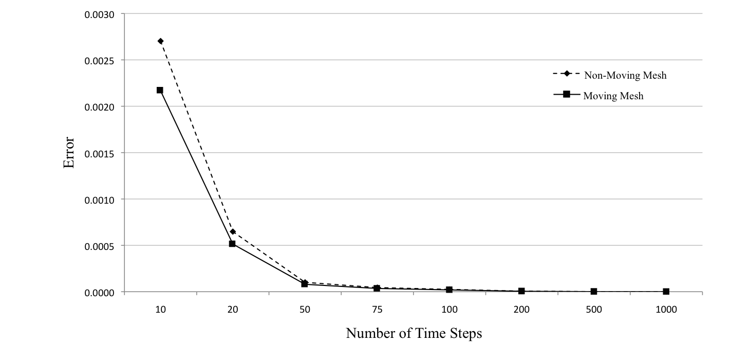
Problem (52) sees a great advantage when the mesh moves with the convection velocity, with up to a 300-fold improvement in the relative error on highly refined meshes with large time steps. The ratio of the final ℒ2\mathcal{L}_{2}-errors of the moving mesh and static mesh solutions at the end of the simulation,

ℒ2−𝑒𝑟𝑟𝑜𝑟=‖u⁡(⋅,1)−u~​(⋅,1)‖0/‖u⁡(⋅,1)−u¯​(⋅,1)‖0,\mathcal{L}_{2}\mathit{-error}=|\!|u(\cdot,1)-\tilde{u}(\cdot,1)|\!|_{0}/|\!|u(\cdot,1)-\bar{u}(\cdot,1)|\!|_{0},

and CPU times are reported in Table 1, where u~\tilde{u} and u¯\bar{u} respectively represent the moving and static mesh solutions. These numbers are relative to the solution computed using a static mesh; values less than 1 correspond to an decrease in the norm of the error or a speedup in the CPU time, when using moving meshes. The accuracy of the solution at the end of the simulation is plotted for n=1001n=1001 with respect to the number of time steps in figure 2.

The greatest gains are realized when Δ​t\Delta t is large relative to Δ​x\Delta x, validating moving finite elements improved stability for larger time steps. However, notice that the use of coarse meshes in space coupled with short time steps leads to unsatisfactory performance. This is caused by large interpolation errors accumulating over many mesh discontinuities. Experiments in [METTITHESIS] demonstrate that these instabilities can be suppressed by using ℒ2\mathcal{L}_{2}-projection, as required by the analysis of Section 3, for such discretizations—since the mesh is coarse in these cases, the speedup from interpolation is rather subtle, which justifies using projection.

n=101n=101 n=501n=501 n=1001n=1001 n=3001n=3001
mm ℒ2\mathcal{L}_{2}-error CPU ℒ2\mathcal{L}_{2}-error CPU ℒ2\mathcal{L}_{2}-error CPU ℒ2\mathcal{L}_{2}-error CPU
10 0.0096 1.018 0.0049 1.009 0.0036 1.007 0.0031 1.014
20 0.0116 1.047 0.0031 1.044 0.0027 1.041 0.0018 1.048
50 0.0235 1.066 0.0031 1.062 0.0019 1.060 0.0016 1.072
75 0.2559 1.067 0.0031 1.059 0.0016 0.576 0.0031 1.063
100 0.0471 1.072 0.0018 1.064 0.0029 0.521 0.0042 1.070
200 4.8120 1.068 0.0304 1.070 0.0036 1.062 0.0065 1.064
500 23.420 1.073 0.0037 1.068 0.0048 1.063 0.0083 1.070
1000 30.122 1.079 3.8142 1.079 0.0047 1.079 0.0087 1.074
Table 1: A comparison table for problem (52) between non-moving and moving mesh methods using interpolation. Reported for each mesh discretization is the ratio of the ℒ2\mathcal{L}_{2}-errors at time t=1t=1 and the relative increase in CPU time of the moving mesh solution to the static mesh solution. Moving the mesh leads to clear advantages when the spatial mesh is sufficiently refined, though buildup in error occurs when the time discretization is too refined, relative to the spatial discretization.

Refer to caption

Fig. 2: The final ℒ2\mathcal{L}_{2}-error at time t=1t=1 of solutions computed for (52) on non-moving (dashed line) and moving (solid line) meshes. The error is significantly reduced using a moving mesh, particularly for larger time steps.

Refer to caption

Fig. 3: A close-up of figure 2. Even for highly refined partitions of the time domain, the moving mesh solution strongly outperforms the static mesh solution.

The next problem we consider is given by

(53) u2,t​(x,t)−((x2+t2+0.1)​u2,x​(x,t))x+0.1​(x3−9​x)​u2,x​(x,t)+u2​(x,t)=f2​(x,t),u_{2,t}(x,t)-\big((x^{2}+t^{2}+0.1)\,u_{2,x}(x,t)\big)_{x}+0.1(x^{3}-9x)u_{2,x}(x,t)+u_{2}(x,t)=f_{2}(x,t),

and the source term and boundary condition are chosen so that the solution of the differential equation is given by

u2​(x,t)=sin⁡(π6​(x+5​t)).u_{2}(x,t)=\sin\Big(\frac{\pi}{6}(x+5t)\Big).

Notice that the magnitude of the diffusion is comparable to the convection velocity, so the effects of the moving elements is primarily to counterbalance the asymmetry of the PDE brought on by the convection term.

A slight advantage is recognized by using moving meshes, when Δ​t\Delta t is not too small relative to Δ​x\Delta x. A comparison of the errors and CPU time is given in Table 2. Comparing the results of this experiment to those of problem (52), it is clear that this problem does not benefit nearly as much from a moving mesh nor is the accuracy as dramatically impacted when the time discretization is much finer than the spatial discretization. Since the diffusion term had a stronger presence in this problem, the solution computed on a non-moving mesh demonstrates comparable accuracy, though small gains come from moving the mesh due to the cancellation of the mesh and convection velocities.

n=101n=101 n=501n=501 n=1001n=1001 n=3001n=3001
mm ℒ2\mathcal{L}_{2}-error CPU ℒ2\mathcal{L}_{2}-error CPU ℒ2\mathcal{L}_{2}-error CPU ℒ2\mathcal{L}_{2}-error CPU
10 0.8012 1.072 0.8014 1.073 0.8014 1.082 0.8014 1.070
20 0.7927 1.068 0.7928 1.075 0.7928 1.053 0.7928 1.071
50 0.7912 1.070 0.7893 1.072 0.7893 1.068 0.7893 1.072
75 0.7946 1.069 0.7888 1.072 0.7888 1.070 0.7888 1.084
100 0.7997 1.071 0.7886 1.072 0.7886 1.060 0.7886 1.066
200 0.8298 1.070 0.7895 1.082 0.7884 1.071 0.7885 1.066
500 0.9405 1.072 0.8009 1.071 0.7908 1.071 0.7883 1.067
1000 0.9791 1.063 0.8387 1.069 0.8010 1.072 0.7884 1.072
Table 2: A comparison table for problem (53) between static mesh methods and moving mesh methods using interpolation. Reported for each mesh discretization is the ratio of final ℒ2\mathcal{L}_{2}-errors and the relative increase in CPU time of the moving mesh solution to the static mesh solution.

Refer to caption

Fig. 4: The final ℒ2\mathcal{L}_{2}-error at time t=1t=1 of solutions computed for problem (53) on non-moving (dashed line) and moving (solid line) meshes. Small gains are made when the mesh moves, especially there are few time steps, as Δ​t\Delta t is large.

In problem (53), setting xt=5x_{t}=5 would move the mesh along the characteristic trajectories of the solution, rather than canceling the convection velocity. This suggests that there are other mesh motion schemes that may improve the accuracy of the computed solution other than the method of characteristics. Other schemes have been proposed that compute the mesh motion and solution as a coupled system of (potentially nonlinear) ODEs, though many of these do not fit into the framework of the moving finite element scheme in Section 3 due to their nonlinearity [CARLSONMILLER1, CARLSONMILLER2]. Other schemes use error estimates [adjerid1986moving1d, adjerid1986moving], predictor-corrector techniques [baines1994moving], and conservation laws to determine the mesh motion [baines2005moving, baines2011velocity]. A mesh motion scheme of primary interest could use a posteriori error estimates and adaptive meshing (hh-refinement at the mesh discontinuities and mesh smoothing to evolve the mesh continuously) to find an appropriate mesh. Such a solver can be implemented leveraging the adaptive meshing routines of some existing software like PLTMG [bank2012pltmg].

One final experiment that we consider is designed to evaluate the moving finite element scheme for a nonlinear problem. We apply our moving space-time method to Burgers’ equation with a large Reynolds number. Burgers’ equation is an interesting test problem for our scheme as it is a simple nonlinear equation that develops steep moving fronts that sweep through the domain. Artificial oscillations are commonly found in the computed solution near the shock layer when the time discretization is not sufficiently refined [MILLER1, MILLER2]. The differential equation given by

(54) ut−1R​ux​x+u​ux=0for⁡(x,t)​in​(−3,3)×(0,2],u_{t}-\frac{1}{R}u_{xx}+uu_{x}=0\quad\mathrm{for}\ (x,t)\ \mathrm{in}\ (-3,3)\times(0,2],

where we choose a large R>0R>0, and we assume Neumann boundary conditions, ux​(±3)=0u_{x}(\pm 3)=0. The initial condition is chosen so that a moving front forms in the middle of the domain and propagates toward the right boundary.

We use the method of characteristics, which gives xt≈ux_{t}\approx u. The solution is computed at the end of each time step so that we can use linear mesh motion xt​(t)=uh​(x,ti−1−)x_{t}(t)=u_{h}(x,t_{i-1^{-}}) for ti−1≤t≤tit_{i-1}\leq t\leq t_{i}. Furthermore, we use a single step of Newton’s method to solve the nonlinear equation at each collocation node. Unlike the earlier experiments, we do not reset the mesh to be uniform at the beginning of each time partition. This allows the nodes to appropriately accumulate near the shock layer, where nodes are deleted once they get too close together. In addition to the standard Galerkin discretizations for the non-moving and moving meshes, we also compare our results to a solution computed using a Streamline Upwind/Petrov Galerkin (SUPG) discretization on a fixed mesh, as in [SUPG].

Figure 5 displays solutions for equation (54) with R=100R=100, computed on fixed meshes with standard Galerkin and a SUPG discretizations in space, where the SUPG coefficient of 0.10.1, as well as a moving finite element discretization. Numerically-induced oscillations are expectedly present in solution found on the non-moving mesh [XUHU], whereas they have already been suppressed in the SUPG and the moving finite element solutions. From figure 5, the moving finite element solution maintains a steep drop into the moving front, where artificial diffusion is clearly present at the top of the shock layer in the SUPG solution. This demonstrates the increased flexibility in the time discretization when moving the mesh, without the artificial diffusion of a SUPG discretization. Experiments combining SUPG and moving meshes give similar results to the standard moving finite element discretization since the “streamline direction,” now given by u−xtu-x_{t}, is small. Figure 6 depicts an example of a moving mesh used for solving the PDE, where we see the spatial nodes accumulating at the shock layer, as desired. We also ran simulations where the Reynolds number is set to R=1000R=1000. This reduces the diffusive forces in the equation and leads to a thinner shock. Solutions computed with 100 time steps are displayed in figure 7, where we again see the moving finite element has remarkably smaller oscillations near the shock layer without the undesirable effects of artificial diffusion.

Fig. 5: Solutions computed for Burgers’ equation with R=100R=100, using n=61n=61 spatial nodes and m=25m=25 time steps. The top graph depicts the solution computed on a non-moving mesh, where oscillations develop near the shock layer. The middle graph plots the solution computed using SUPG, using a SUPG coefficient of 0.10.1. The bottom graph shows that the moving finite element solution has successfully dampened these spurious oscillations. In comparing the moving finite element solution with the solution computed using SUPG, the moving finite element solution maintains a steeper shock layer, whereas artificial diffusion has smeared the layer in the SUPG solution.

Refer to caption

Fig. 6: An example of a moving mesh with m=25m=25 time steps and initialized with n=61n=61 spatial nodes at the beginning of the simulation. The method of characteristics sets xt≈u⁡(x)x_{t}\approx u(x), where both the hat and bump node trajectories are depicted. Comparing the density of the spatial nodes to the figures of the computed solutions in figure 5, the spatial nodes properly congregate near the shock layer and track it throughout the simulation.

Fig. 7: Solutions computed for Burgers’ equation with R=1000R=1000, using n=301n=301 spatial nodes and m=100m=100 time steps. The top graph depicts the solution computed on a non-moving mesh, where large oscillations develop near the shock layer. The middle graph shows the solution computed using SUPG, where the SUPG coefficient is set to 11. The top of the shock layer in the solution computed using SUPG is not sharply defined and small oscillations are present at its foot. The bottom graph shows that the moving finite element solution has almost completely dampened these spurious oscillations, while preserving the sharpness of the solution on both sides of the shock layer.

5 Conclusion

Theorem 4.3 of [BANKMETTI] provides a symmetric error bound for some space-time moving finite element methods that use a one parameter family of collocation methods. Employing TR-BDF2 for time integration, however, does not fit into this framework and complicates the analysis of this finite element method, ultimately breaking the symmetry of the error bound. Nevertheless, it has been shown that Theorem 4 analytically implies second order accuracy with respect to mesh refinement [METTITHESIS] and the moving finite element scheme yields superior performance over the method of lines approach with a stationary mesh, as demonstrated by the numerical results. Furthermore, improved accuracy for the moving finite element solution was maintained in application to a simple nonlinear problem, although the theoretical analysis does not cover such cases.

In the numerical experiments, the method of characteristics was used to determine the mesh motion; however, an optimally robust and well-defined mechanism for evolving the mesh for general PDEs is still a matter of active research. It is suspected that predictor-corrector methods, coupled with adaptive meshing for the spatial discretization, can be powerful tools in moving the mesh without requiring additional user-supplied information about a PDE or its solution.