JLAB-THY-13-1814, CFTP/13-026
Confinement, quark mass functions, and spontaneous chiral symmetry breaking
in Minkowski space
Abstract
We formulate the covariant equations for quark-antiquark bound states in Minkowski space in the framework of the Covariant Spectator Theory. The quark propagators are dressed with the same kernel that describes the interaction between different quarks. We show that these equations are charge conjugation invariant, and that in the chiral limit of vanishing bare quark mass, a massless pseudoscalar bound state is produced in a Nambu–Jona-Lasinio (NJL) mechanism, which is associated with the Goldstone boson of spontaneous chiral symmetry breaking. In this introductory paper we test the formalism by using a simplified kernel consisting of a momentum-space -function with a vector Lorentz structure, to which one adds a mixed scalar and vector confining interaction. The scalar part of the confining interaction is not chirally invariant by itself, but decouples from the equations in the chiral limit and therefore allows the NJL mechanism to work. With this model we calculate the quark mass function, and we compare our Minkowski-space results to LQCD data obtained in Euclidean space. In a companion paper we apply this formalism to a calculation of the pion form factor.
pacs
11.15.Ex, 11.30.Rd, 12.38.Aw, 12.39.-x, 14.40.-nI Introduction
The connection between the mass spectrum and structure of hadrons and their underlying internal gluon-quark dynamics is today an important and challenging problem in physics. At the heart of forthcoming experimental programs at for instance JLab and FAIR, and of the immense progress in lattice QCD (LQCD) calculations [1, 2] lies the identification of hybrid baryons, exotic and hybrid mesons, as well as the understanding of the full implications of dynamical chiral symmetry breaking. At present, models are necessary to establish a link between LQCD calculations and experimental data.
Furthermore, today a believable model must go beyond the extensive work of Isgur and Godfrey [3] and Spence and Vary [4]. These models might be adequate for heavy-quark systems well described within a nonrelativistic framework, but mesons containing at least one light quark require a fully relativistic treatment. It is therefore desirable for a unified description of all quark-antiquark states to use a bound-state equation that is both Lorentz covariant and that reduces to the Schrödinger equation in the non-relativistic limit. In addition, these earlier quark models ignored chiral symmetry breaking and used static potentials (often variations of the very successful Cornell potential [5, 6, 7]) to describe the interaction between constituent quarks with a fixed mass.
Non-perturbative methods, including numerical solutions of QCD on a discrete space-time lattice and of the modern Dyson-Schwinger and mass gap equation [8, 9, 10, 11, 12, 13, 14, 15, 16, 17, 18, 19, 20, 21, 22, 23], have developed tools which unify the explanation of a wide range of meson and baryon phenomena [24, 25, 26]. A key feature of these approaches is the emergence of a dynamical description of a constituent quark which can acquire, through dynamical chiral symmetry breaking, a momentum dependent mass function leading to an effective constituent quark mass which can be much larger than the current-quark mass. It is now possible to discuss the structure of the constituent quark, or how, in the chiral limit, the spontaneous generation of a constituent quark mass is linked to the existence of the pion bound state with zero mass through the famous NJL mechanism. This connection is both interesting and an essential ingredient to our understanding of the light meson spectrum. Without it, the light pion mass appears to be an accident resulting from fine-tuning of the interaction parameters.
A covariant treatment of mesons including the NJL-mechanism can be found in the papers by C. D. Roberts and his collaborators, (see for example [27] and [28] and references therein), based on the Dyson-Schwinger equation, which we denote by DSE. The work presented here starts from a physical model of dynamical quarks and mesons similar to that assumed by the DSE, but it differs in two important aspects: (i) we work in Minkowski space instead of Euclidean space, and (ii) we include a Lorentz scalar confining interaction. Both of these differences are significant and have their own advantages.
Aspect (i) is important because, while some observables can be calculated just as well in Euclidean space as in Minkowski space (particle masses, for example), others, such as transition form factors in the timelike region, require a framework defined in Minkowski space. Aspect (ii) enables us to address an important question: although phenomenological approaches and lattice calculations may suggest that the confining force is scalar, those indications are not definitive [29, 30, 31, 32, 33, 34, 35], and while DSE suggests that confinement is not important to (and maybe even absent from) the light meson spectrum, it is clearly an advantage to have an approach that is flexible enough to allow the confining interaction to be present (and to investigate the relative strengths of scalar and vector components). This is certainly possible in the approach that is developed in this paper. As it turns out, the scalar confining interaction, when its relativistic extension is adequately defined, decouples in the chiral limit, allowing the NJL mechanism to work. Therefore the breaking of chiral symmetry by such a scalar component does not constitute a problem in our formulation. This remarkable fact will be discussed in some detail in this paper.
This work extends and improves upon early work done by Gross and Milana [36, 37, 38], and Şavkli and Gross [39], denoted collectively by GMS. The Covariant Spectator Theory (CST) [40, 41, 42] already used in GMS, was extensively tested in the treatment of nucleon-nucleon scattering [43, 44] and pion nucleon scattering [45, 46]. This paper improves on GMS and prepares the way for subsequent studies of the structure of all mesons, planned for future papers. The formulation shown in this paper differs from previous CST models in the sense that the mass function is calculated by solving the one-body CST-Dyson equation, directly from the same kernel entering the two-body CST-Bethe-Salpeter equation. This makes our model completely self-consistent and in line with the traditional Dyson-Schwinger approaches. Other advances presented here are: (i) the proof of chiral symmetry breaking in a charge-conjugation symmetric CST four channel formulation, (ii) a new extended definition of the relativistic kernels that is needed when both particles are off-shell, essential for some applications.
Before turning to the details of the model, we remind the reader of an essential feature of the CST approach: quarks can have real mass poles and can be on their mass-shells. Confinement is achieved by constructing an interaction that guarantees that two or more quarks cannot be on-shell together. The alternative view is that confinement occurs because the quark propagator does not have any real mass-shell poles. For those who find the concept of an on-shell quark distasteful, it may help to think of the on-shell quark as a effective degree of freedom that is not physical, since, unlike nucleons (for example), quarks can never be isolated and can never be observed. The issue is whether or not such an effective degree of freedom is useful in explaining the phenomena of QCD; until it is developed and tested a definitive answer cannot be given. A feature of this picture of confinement of quarks is that it is similar to the usual nonrelativistic picture, allowing us to make comparisons with nonrelativistic models.
In Section II we motivate and write the charge-conjugation-invariant CST four channel equations. In Section III we focus on the equations for the pseudoscalar bound state. In Section IV we prove that in the chiral limit the one-body CST-Dyson equation coincides with the two-body CST-Bethe-Salpeter equation corresponding to a zero mass Goldstone boson. Section V describes the general form of the CST kernel. The results for the quark mass function and their connection to LQCD are shown in Section VI. Section VII summarizes and describes our conclusions.
A companion paper (prepared at the same time) uses the results of this paper to calculate the pion electromagnetic form factor [47]. It is referred to as Ref. II.
II Charge conjugation invariant equations for quark-antiquark bound states
II.1 Background
The purpose of this section is to motivate the structure of the equations used in this and forthcoming papers. The details of the interaction kernel are not of importance at this stage and will therefore be specified later in Section V.
We begin by clarifying and reviewing the relation between the Bethe-Salpeter (BS) [48] and the CST equations. The CST equations can be conveniently obtained from the BS equations by integrating over the internal energy variables and retaining only the contributions from certain propagator poles (for a two-body equation for non-identical particles with unequal mass, only the heavier particle pole is retained). While this is a convenient technique for obtaining the equation, one might conclude from it that the CST equation is merely the result of an approximation of the BS equation. Unfortunately, this interpretation misses the key point, namely that the omission of the poles of the kernel or other propagators reflects, in some cases, cancellations between various parts of the complete kernel and its iterations, in particular between ladder and crossed-ladder diagrams. One has to keep in mind that an exact BS kernel contains an infinite set of irreducible diagrams, which has to be truncated in practical calculations. When using a truncated kernel (usually a ladder truncation), omitting its poles can actually yield a better approximation to the exact BS equation (i.e., with a non-truncated complete kernel) than keeping them. This surprising observation plays a central role in the CST framework. Furthermore, the CST equations are manifestly covariant (in common with the BS equations) and, even when used with a truncated kernel (the ladder sum, for example), have a smooth nonrelativistic limit (not usually a feature of the BS equation with a truncated kernel). A brief review of the foundations of the CST and its many applications can be found in Ref. [49].
A unified description of all mesons composed of quark-antiquark pairs requires a bound-state equation that transforms correctly under charge conjugation: the equation for a bound-state particle should transform into the equation for the bound-state anti-particle. In particular, both the vertex function and its charge conjugate must satisfy the same equation. For instance for the case of the pion, the vertex functions for both and , which are connected by charge conjugation, should be the solutions of the same bound-state equation.
We begin the discussion of charge conjugation symmetry with the BS equation, which is manifestly covariant and naturally satisfies charge conjugation symmetry. As outlined above, the CST equation can be obtained from the BS equation by keeping only certain propagator poles of the BS integrand. As a consequence of the omission of some of the propagator poles, the CST equations are not automatically charge conjugation symmetric. In most cases where this framework has been applied so far, in particular in the description of few-nucleon systems, charge conjugation invariance is not an important issue. But for this paper, where we want to deal in particular with quark-antiquark systems of equal-mass quarks, it is important. In this section, charge conjugation invariance is restored by symmetrizing the equations, leading to a system of four coupled equations [39]. These are the “four-channel CST equations.”

II.2 Bethe-Salpeter equation
The BS vertex function is denoted , with the four-momentum of the outgoing quark and the four-momentum of the outgoing antiquark (diagrammatically represented as an incoming quark of momentum ). is the bound-state four-momentum and and are the intermediate four-momenta of the quark and antiquark, respectively. With this notation the BS equation for the vertex function, shown diagrammatically in Fig. 1, is written
| (1) | |||||
Here is the interaction kernel, which is an operator in the color and Dirac spaces of the two quarks whose interaction it describes. It is written in the general form
| (2) |
where and are Dirac matrices of type at the vertex involving quark 1 and 2, respectively, and the are covariant scalar functions describing the corresponding momentum dependence. It is convenient to write the kernel in terms of the relative momenta and the total momentum instead of the individual particle labels, , etc. How this kernel acts as an operator in Dirac space can be seen by following along a fermion line in Fig. 1:
| (3) |
The color SU(3) generators are given in terms of the Gell-Mann matrices, . Mesons are color singlet states, for which
| (4) |
The factor of in (2) has been factored out in order to cancel this color matrix element. Color degrees of freedom can then be effectively ignored and will no longer be referred to in the remainder of this work.
The dressed quark propagator, (with the factor of removed), is given by
| (5) |
with the bare mass and the self-energy of the quark, of the form
| (6) |
If the quark and antiquark have the same bare mass and identical self interactions, the particle label on can be dropped,
| (7) |
Charge conjugation, denoted by the operator , transforms quarks into antiquarks and vice versa, accomplished by taking the transpose of the vertex function and changing . The amplitude is invariant under charge conjugation if it remains unchanged up to a phase , with . The required condition is therefore
| (8) |
Performing this operation on Eq. (1), and using and the charge conjugation invariant conditions
| (9) |
where implies . This gives
| (10) | |||||
which shows that satisfies the same equation as (and hence the two are equal up to a phase), provided conditions for the propagators and kernel, Eqs. (7) and (9), are satisfied. We will always choose kernels that satisfy condition (9).
Note that a crucial step in the derivation was our ability to change the four-dimensional integration variable . This condition must be preserved when we specialize to the CST.

II.3 Charge conjugation invariant CST equations
Next we introduce a charge-conjugation invariant form of the bound-state CST equations. For cases when we want the correct limit as these are the “four-channel” equations previously discussed [39].
To motivate the structure of these equations, begin with the BS equation (1) and consider the integration. The dressed propagator of quark with dressed mass and renormalization constant can be written
| (11) |
near its poles at , where . Here we ignore the running of the dressed quark mass for the time being, but it will be included later. Figure 2 shows the positions of the four propagator poles in the complex plane in the bound-state rest frame (note that here is the zero component of the relative momentum , not of the individual particle momenta ). In the rest frame, the total momentum is , the quark and antiquark three-momenta are equal to the relative three-momentum , and therefore , with . However, in the following we will continue working in an arbitrary frame with total momentum in order to emphasize the manifest covariance of our framework.
To perform the integration we can close the contour in the lower or upper half plane. In the CST framework only poles of propagators are included, whereas the poles of the kernel are moved to higher order kernels, which are usually neglected. As one can see in Fig. 2, in either half plane the respective two poles are separated by the bound-state mass . If is large, the pole closer to the origin dominates the integral, and the more distant pole can be neglected. However, in the limit the two poles move close together and the contributions of both must be taken into account.
First we close the contour in the lower half plane. Introducing the on-shell momenta permits the two propagator pole contributions to the right hand side of (1) to be written
| (12) | |||||
where is the dressed propagator including the self-energy, and the positive-energy projection operator is
| (13) |
and, for any , the integral is abbreviated as
| (14) |
Note that the notation used here for with the self-energy is the same as in the previous section, but these are now CST objects and are not identical to their BS analogues. For the remainder of the paper, they will always refer to CST quantities, unless otherwise stated.
Equation (12) can be simplified by renaming the integration variables and using the shorthand notation to denote the four-momentum of whichever particle is on-shell (so that, from this point on, now denotes the three-momentum of the on-shell particle)

| (15) |
We will now address the issue of charge conjugation symmetry of the CST bound-state equation. The equation just obtained is not charge conjugation invariant because it includes no poles from the upper half complex -plane, necessary for the symmetry used in the proof. To correct this, we symmetrize the contributions from the contour in the lower half plane and the upper half plane, as illustrated in Fig. 2, which effectively amounts to taking their average.
In the upper half plane, the sign for the energies is reversed. Guided by the argument used for the BS equation, we will also change the sign of the integration three-momentum , so that . The right hand side of the CST equation for the BS vertex now contains four terms (which will lead to the four-channel CST equation). To simplify the notation, the kernel will be written , with the dependence on the total momentum understood, and we use the following abbreviations for the four amplitudes
| (16) |
With this simplification, the equation becomes
where we have replaced by in the last two terms under the integral such that the negative-energy on-shell four-vector becomes equal to . Note that the first and third, and the second and fourth terms differ only by , preserving the symmetry required for charge conjugation invariance. Equation () is diagrammatically depicted in Fig. 3, and we will refer to it as the CST-BS equation. It expresses an approximate BS vertex function in terms of the CST vertex functions. Once the latter are known, it can be used to define a CST vertex function for states in which both quark and antiquark are off mass shell. But in order to determine the CST vertex functions in the first place, Eq. () needs to be converted into a closed set of four coupled equations, which is achieved by writing () for each of the four values of the relative momentum where is a individual quark on-shell momentum. Introducing the 16 kernels
| (18) |
where a subscript (with ) indicates that quark is on its positive or negative energy shell, respectively. Note that a negative-energy quark should be interpreted as the corresponding physical positive-energy antiquark. With this notation the four equations become
| (19) | |||||
The system of equations (19) is the four-channel CST equation.
III Equations for the pseudoscalar bound state
The pion as the lightest of the mesons requires a treatment consistent with chiral symmetry. In particular, we will show that, in the chiral limit of vanishing bare quark mass , the pion bound state mass also tends to zero, while the constituent quark mass acquires a finite value due to its dressing through the interaction kernel. Our demonstration will be done in two steps:
In this section, we apply the four-channel CST equations (19) to the case of a pseudoscalar bound state and perform the limit. Then, in the next section, the resulting equation is shown to be consistent with the one-body CST-Dyson equation (i.e. the equation for the quark self-energy) in the chiral limit. This property is essential for the existence of a zero-mass pion solution, which plays the role of the Goldstone boson associated with the spontaneous breaking of chiral symmetry.
III.1 General results
The most general form for the BS vertex function for a pseudoscalar bound state can be written
| (21) |
where , , and are scalar functions. If the state is invariant under charge conjugation with a phase , then the relation (8), together with , , and , leads immediately to the conditions
| (22) |
Using the decomposition (21), the CST amplitudes (16) are
| (23) |
where . The vertex functions (23) satisfy the charge conjugation conditions (). Substituting the definitions (23) into () and writing the result in the form (21) gives four equations for the scalar BS vertex functions of the pion in terms of the CST vertex functions, which can be computed by substituting (23) into (19). We will not pursue these general relations at this time; instead we look at the mass zero limit of the pion bound-state equation.
III.2 Zero-mass limit
For this case it is advantageous to go first to the bound-state rest frame where , and then perform the limit . In the rest frame the vertex functions (23) become
| (24) |
It will be shown shortly that the zero-mass limit of the BS vertex function for the pion can be obtained from the zero-mass limit of the pion CST vertex functions (24). Since the pion is even under charge conjugation (), when , and all of the vertex functions reduce to a single function, which will be denoted , with
| (25) |
where . Substituting this into () for the BS vertex function gives
| (26) |
where
| (27) |
Here the limit has been taken everywhere but in the propagators, where the numerators and denominators are both of order , canceling to give a finite result in the limit.
To work out this limit and to evaluate , use the general form (5) of the dressed propagator, which can be written
| (28) |
where the mass function is
| (29) |
and is the wave function renormalization, and , , and are functions of . The dressed mass is defined by the condition
| (30) |
with and . Similarly, we define . With our application in mind, we expand the propagators about the energy of the four-vector , with and
| (31) |
Expanding and the mass function about (to order is sufficient) gives
| (32) |
where
| (33) |
(with and defined similarly). To order the dressed quark propagator becomes (with for use with the first two terms in (26) and for use with the last two)
| (34) | |||||
where is the renormalization constant. The singular term and the correction cancel when inserted into [because ], leaving finite terms
| (35) | |||||
Inserting this into (26) gives finally
| (36) | |||||
Using the representation (2) for a particular kernel with Lorentz scalar and vector couplings,
| (37) |
shows that
| (38) | |||||
Since , this equation has a non-zero solution only if
| (39) | |||||
This equation is the condition for the existence of a massless solution of the pion bound-state equation and will be referred to as the massless pion condition.
IV Chiral-symmetry breaking in the CST
In the GMS model the spontaneous breaking of chiral symmetry is realized through the famous NJL-mechanism: In the chiral limit of vanishing bare quark mass chiral symmetry is dynamically broken by a finite dressed quark mass that is spontaneously generated by the self-interactions of the quark through the interaction kernel. This symmetry breaking is accompanied by the existence of a zero-mass pseudoscalar bound-state, the Goldstone pion: It can be shown analytically that the one-body CST-Dyson equation for the scalar self-energy becomes identical to the two-body CST-BS equation for a massless pion as . Therefore, the existence of the solution for one implies a solution for the other. On the other hand, away from the chiral limit, the existence of a solution of the one-body equation ensures that there cannot exist a massless-pion solution of the two-body equation at the same time.
In this section we derive the condition for the scalar part of the CST one-body equation to have a non-trivial solution and therefore to generate a contribution to the dressed quark mass. In the chiral limit this condition reduces to (39) which guarantees the existence of a massless pion, and at the same time ensures that the pion is not massless for finite bare quark masses. It will be seen that for this mechanism to work the interaction kernel must satisfy certain conditions. In particular, for the case of the kernel of Eq. (37), must not contribute to either the one-body equation for the scalar self-energy or to the two-body equation for a massless pion.
IV.1 Mass functions
Using the kernel (2), the BS self-energy
| (40) | |||||
is given from the four-dimensional one-body Dyson equation diagrammatically depicted in Fig. 4. (Here, since , the and are individual quark off-shell four-momenta.)

In the CST, we are instructed to take an average of the contributions from the quark pole in the lower half plane, where the singularity is at , and the upper-half plane where the singularity is at , see Fig. 2. The corresponding one-body CST-Dyson equation is diagrammatically depicted in Fig. 5.


Calculating these pole contributions from the singular (first) term in the expansion (34), and changing in the negative energy term (so that ) gives
| (41) |
Inserting the kernel (37) we obtain
| (42) | |||||
For simplicity, evaluate this in the rest frame (), where the integral over ensures that , and extract the self-energy functions and
| (43) | |||||
Note that, since , and are functions of , as required by Lorentz covariance.
At (so that ), the constraint (30) gives
| (44) |
Using this reduces the equation for at to the constraint
| (45) | |||||
Comparing Eqs. (39) and (45) shows that they are identical if and if the integral over the scalar interaction vanishes:
| (46) |
This condition is satisfied by the models discussed in this paper.
Unless , constraint (39) will not be satisfied, insuring that there is no pion bound state with zero mass. This means that the same constraint that makes it possible that [Eq. (45)] also ensures that there exists a pion with zero mass [Eq. (39)] in the chiral limit. These consistency conditions link the spontaneous generation of a dressed quark mass in the chiral limit, and hence the spontaneous breaking of chiral symmetry, to the existence of a massless Goldstone pion.
The equivalence between the zero-mass pion equation and the self-energy equation in the chiral limit can also easily be demonstrated in terms of Feynman diagrams, as shown in Fig. 6: The scalar self-energy becomes equal to the scalar part of the inverse dressed propagator in the chiral limit. Multiplying with a , attaching two off-shell quark lines of momentum and one pion line of zero momentum yields a “spacelike” Yukawa vertex. Then, crossing symmetry allows to switch to the “timelike” creation/annihilation channel, which is equivalent to the (approximated) BS pion vertex function (expressed in terms of CST functions) in the chiral limit. This shows that, in the chiral limit, the scalar part of the quark self-energy, , is equivalent to , the BS vertex function for an off-shell outgoing quark and antiquark with momenta and , respectively.
A word of caution about the interpretation of Fig. 6 is in order: while the drawing shows that the two internal quarks are both on-shell at the same time, this contribution does not correspond to quark-antiquark scattering. As already shown in (35), the singular part of the dressed propagator, which is the only part that would contribute to true scattering and deconfinement [39], cancels. Hence the contribution to the diagram is the finite, non-singular part, not associated with any propagation of the quarks.
V General definition of the kernel
Our discussion so far on charge conjugation and chiral-symmetry breaking applies to all covariant interaction kernels of the form (37) that satisfy the symmetry property (9) together with the condition on the scalar part , Eq. (46). In this section we specify the momentum-depended parts of the kernel. They include confinement and they are manifestly covariant expressions with the correct nonrelativistic limit, a property crucial for a unified description of all mesons.
V.1 The relativistic kernel
The kernel we use is a relativistic generalization of the nonrelativistic potential
| (47) |
which is the superposition of a linear confining interaction, , and a constant interaction, . For a particular choice of the parameters and , this potential is similar to the very successful Cornell potential [5, 6, 7] used for the description of the charmonium spectrum. The constant interaction is used for simplicity. It can be replaced by a color-Coulomb potential if needed.
A proper CST generalization of (47) to be applicable to the four-channel equations () must include the condition that either the quark or the antiquark are on-shell in the initial state. The kinematics for these two terms is illustrated in Fig. 7.
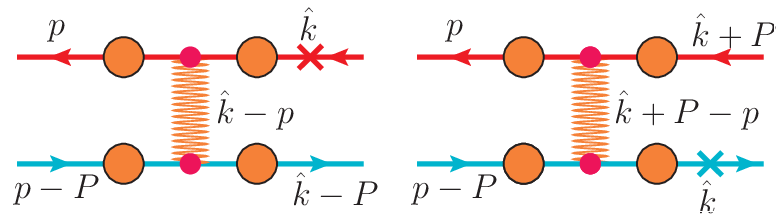
The covariant kernels in momentum space will be denoted as and . In the rest frame of the bound state, where , the operation of the confining part on any regular function will be defined by the result
| (48) |
where, if the momenta are labeled as in Fig. 7, with and , then the kernel in the left panel is
| (49) |
The ’s are dimensionless strong quark form factors to be discussed in Section V.3. The two cases and are called “diagonal” and “off-diagonal” parts of the kernel, corresponding for on-shell to the left and right panel in Fig. 7, respectively. The fact that (48) does indeed describe a linear confining interaction in the non-relativistic limit has been extensively discussed [36, 39].
The “constant” part of the kernel, , is defined by
| (50) | |||||
where
| (51) | |||||
and is the dressed quark mass. Note that the sign in (51) is consistent with the sign in the nonrelativistic limit (47) because a vector interaction changes sign when taking the nonrelativistic limit [50].
The factor of contained in the volume integrals used in (48) and (50) ensures that the three-dimensional volume integrals are covariant (because is the three-momentum of an on-shell quark of mass ), so that the whole expression is covariant if the ’s are covariant. They also ensure a smooth transition to the nonrelativistic limit when . The subtraction term, , is an improved version of the one proposed in Ref. [36], with the subtraction generalized to properly regulate both the “diagonal” singularities of at and the “off-diagonal” singularities at . The argument of the subtraction term is , with the value for at which becomes singular. For instance, for and (which occurs in the evaluation of the quark self-energy in the quark rest frame – see Sec. VI), we have
| (52) |
The subtraction term has two important functions: (i) it regularizes the singular confining kernel , reducing it to a unique and well-defined Cauchy principal value integral, and (ii) it ensures that the relativistic generalization of the nonrelativistic condition , written in momentum space
| (53) |
is satisfied.
Although the covariant interaction kernel has been constructed in such a way that it reduces to the linear confining potential in the nonrelativistic limit, it is a priori not obvious that it actually confines. As already mentioned in the Introduction, there are, in principle, two ways confinement can be realized: (1) the dressed propagators have no real quark mass poles, or (2) the bound-state vertex function vanishes as two or more quarks are simultaneously on-mass-shell. It has been proven in Ref. [39] that the latter realization of confinement applies to the CST approach. For this to work out the subtraction term in Eq. (48) is crucial as it becomes singular when both quarks are on-shell, which forces the vertex function to vanish, for consistency.
This concludes our discussion of the momentum-dependent parts of the kernel and we turn now to its Lorentz structure.

V.2 Lorentz structure of the kernel
An appealing feature of the GMS model is the property that the linear confining interaction does not contribute to the CST equation for a massless pseudoscalar bound state [37]. This can immediately be seen from Eq. (38) by inserting for and in the kernel and using condition (53). The same applies to the CST equation for the scalar self-energy , Eq. (43). Therefore,
| (54) |
and hence the linear confining interaction does not contribute to the generation of a dressed quark mass. This decoupling of confinement from chiral symmetry breaking permits our confining potential to have a Lorentz structure that includes, e.g., a Lorentz-scalar coupling part as suggested from phenomenological approaches [29, 30, 31] and LQCD calculations [32, 33, 34, 35]. Specifically, we employ a mixture of scalar and vector coupling, where is the mixing parameter:
The relative minus sign between scalar and vector parts guarantees that the kernel evaluated between on-mass-shell spinors for the quarks and antiquarks yields the correct potential (47) in the nonrelativistic limit, without renormalizing its strength .
Unlike the confining interaction, the constant interaction does contribute to the equation for a zero-mass pseudoscalar bound-state. This constrains its Lorentz structure to be chirally symmetric. There are several possible choices, however not all of them also yield a zero-mass pion in the chiral limit [36]. In particular, if one allows only Lorentz scalar and vector structures as in (37), then condition (46), which must be satisfied in order to have dynamical chiral-symmetry breaking, requires the scalar part to vanish. Therefore we assume a pure vector structure for the constant interaction, which, in arbitrary color gauge and using the conventions of Eq. (37), is written
| (56) | |||||
where was defined in Eq. (51). Here is the gauge parameter. The choice corresponds to the Feynman gauge and to the Landau gauge. The constant included in will be chosen to be consistent with chiral symmetry and to give a reasonable description of the quark structure.
V.3 Strong quark form factors
The kernels given in Eqs. (48) and (50) include (strong) phenomenological form factors [51, 52, 38, 46]. Their purpose is twofold: they can be regarded as describing some gluonic corrections to the vertices that would otherwise be overlooked, and they provide convergence in loop integrals. The form factors are expressed as products of individual quark form factors , one for each quark line associated with momentum .
The idea that these form factors serve as an effective description of the infinite sum of overlapping gluon loop corrections to the interaction vertices is illustrated in Fig. 8 (shown only for two-loops). This raises the possibility that they could be calculated from first principles at a later date.
The explicit form of will be specified later. Our quark form factors differ from those used in previous approaches by their normalization at the on-shell point . They will be normalized to 1 only in the chiral limit, , and therefore . With this normalization all free parameters of the quark mass function are fixed in the chiral limit and the constituent quark mass for finite is then uniquely determined from the mass constraint (30).
The use of factorized form factors [where the form factor at a vertex, , is separated into a product of separate form factors, ] is an advantage when calculating electromagnetic current matrix elements in the presence of strong form factors. If they are moved from the vertices to the quark propagators (leaving the vertices bare) as illustrated in Fig. 9, and reinterpreted as an additional correction to the quark propagator, then a dressed quark current can be constructed that includes them and also satisfies the Ward-Takahashi identity [51]. This is discussed in Ref. II.
VI Quark mass function
In this section we apply the interaction kernel defined in the previous section to calculate the CST self-energy given in Eq. (43), and consequently the dynamical quark mass function from Eq. (29). Our Minkowski-space results are then compared with LQCD calculations performed in Euclidean space. This comparison requires the computation of our mass function at negative values of .
VI.1 Self-energy from the linear confining potential
The discussion on the decoupling of confinement from chiral symmetry breaking revealed that the linear confining potential does not contribute to the dynamical quark mass generation because the corresponding contribution to the scalar self-energy vanishes, as expressed in Eq. (54). For the remaining vector part of the self-energy we insert the confining kernel (48) into Eq. (43) and get
| (57) | |||||
where the form factors discussed in Sec.V.3 have been introduced at each vertex. Equation (57) shows that is a function of , as it should be. Note that this would not be the case if we had not included the negative-energy propagator-pole contribution from the upper half complex -plane. Furthermore, (57) displays the simple dependence of on the adjustable mixing parameter . For the particular choice , is zero and the confining potential does not contribute at all to the quark self-energy, i.e.,
| (58) |
This choice corresponds to a ratio between scalar and vector coupling in the Lorentz structure of the confining kernel.
The case is appealing because of its simplicity as it avoids the computation of the UV-divergent integral in (57), and therefore we will explore this case in the remainder of this work. However, in future work we will compute the integral (57) using Pauli-Villars regularization, and will be determined through a fit to the meson spectrum. It appears unlikely that should emerge automatically from such a fit, and we expect that the confining interaction will then actually contribute to the quark self-energy.

VI.2 Self-energy and mass function from the constant interaction
Next we look at the self-energy contribution from the constant potential of Eq. (56). Returning to Eq. (41), in the rest frame of the quark, where its four-momentum is , we find
| (59) | |||||
where has been evaluated using Eqs. (50) and (56), (see below), and is the gauge parameter taken from (56). Equation (59) also shows that
| (60) |
because the two pole contributions cancel. This result implies that a wave-function renormalization factor can only originate from the confining interaction. However, since we chose , the confining interaction does not contribute to the self-energy at all and , as assumed above. This fact has to be kept in mind when our mass function for is compared to LQCD calculations, such as the ones of Ref. [53], where the mass function contains an overall factor substantially smaller than 1 at low .
The mass function is not a physical observable and depends on the choice of the color gauge. In our case, this is explicit in Eq. (59) through the term containing the gauge parameter . The gauge dependence is very simple, and any change in the gauge parameter can be absorbed into the coupling constant through the redefinition
| (61) |
In the Feynman gauge we have , whereas in the Landau gauge . We will work in the Feynman gauge, so the mass function (29) becomes
| (62) |
The coupling constant is not a free parameter but constrained by the mass condition (30). In the chiral limit (), which we indicate by a subscript , the constraint is
| (63) |
We choose , fixing the constant at
| (64) |
Away from the chiral limit (), we expand around :
| (65) |
where is a constant. For sufficient small we keep the first order term only. Then the mass condition becomes
| (66) |
which determines the dressed mass in terms of the quark form factor . The coefficient will be chosen in Section VII in order to give a reasonable fit to the existing LQCD data.
The final result for the dressed quark mass function is
| (67) |
which reduces in the chiral limit to
| (68) |
This mass function incorporates asymptotic freedom correctly: in the ultraviolet limit the quark mass approaches the bare quark mass , i.e.,
| (69) |
On the other hand, in the infrared region the constituent quark mass is generated from the dressing through the interaction kernel. Even in the chiral limit of vanishing bare quark mass a finite constituent quark mass is generated dynamically. In the present simple model for the interaction kernel where the Lorentz scalar-vector mixing in the confining interaction has been chosen such that there is no contribution to the self-energy, the dressing of the quark is entirely determined in terms of the quark form factors at the interaction vertices.
To counter any impression that the mass function is purely phenomenological we point out that it acquires the simple form (67) only in the present special case of a Lorentz scalar-vector mixing for the confining interaction. If there is a non-trivial influence from the confining interaction on the mass function, reflected in a wave function renormalization . Furthermore, the mass function (67) is the solution of the one-body CST-Dyson equation of Eq. (42) when the simple interaction kernels discussed in Sections V.2 and V.3 are used. In this model, it is the kernel that is phenomenological, with parameters fixed by data and lattice calculations as discussed below.
VII Results and discussion
We take a simple form for the strong quark form factors ,
| (70) |
with and where is an adjustable mass parameter. This form for guarantees that there will always be one and only one mass solution of the gap equation. has to be chosen such that the pion form factor calculation described in Ref. II converges, which requires . In this work we choose .
Note that has a pole at . This point lies far outside of the region of interest, but it may still be worthwhile to point out briefly how this result could be improved. One possibility is to choose a function of the form
| (71) |
and . This function is symmetric about and the pole at is removed. We leave further discussion of this for another time.
The mass function in the chiral limit, Eq. (68), involves two free parameters, the chiral constituent quark mass and . The constituent quark mass is obtained by solving the mass condition, Eq. (66), for finite bare quark masses . We fix our mass-function parameters using the LQCD data [53], with four data sets for the bare quark masses and GeV. Since the lattice data are calculated in Euclidean space, they must be compared with the Minkowski-space calculation at negative . To carry out the fit the four sets of lattice data are extrapolated to zero bare quark mass by a linear fit, and then and are determined from a fit of the chiral mass function (68) to these (extrapolated) chiral-limit lattice data. Only the lattice data points at small values of (in particular, the first 50 points between and ) are used in the fit. The reason for not using all available lattice data is that the ultraviolet tails of the data do not approach the corresponding values of the bare quark mass, a deviation from the correct asymptotic behavior attributed to an insufficiently small lattice spacing [54], whereas the finite lattice spacing effects are expected to be small for the lower 50 points. This procedure gives a chiral constituent mass of and a mass parameter . The corresponding mass function is plotted in Fig. 10.

To test our parameter-fixing procedure, the mass functions for the bare quark mass values and GeV have been determined by finding the dressed masses for these values of using the gap equation (66), and comparing the results with the corresponding lattice data. With a value for the expansion coefficient in a good fit to the lattice data at small negative is achieved (fitting the data points up to with an overall ), as shown in Figs. 11 and 12.


For small near the chiral limit and for small our results are in good agreement with the lattice data. As becomes larger a deviation from the lattice data is observed not only in the perturbative region of large (due to finite lattice-spacing effects as mentioned above) but also at small . The fits using only 50 lattice data points seem to give slightly better agreement with the data for large than a fit of more points up to larger values of . In particular, it is interesting to observe in Fig. 12 that for large , the lattice data at small seem to lie slightly above our results. This might be attributed to the fact that with we have , which does not agree with the lattice data at small values of .
Certainly, there exist various functional choices for the form factor that would give a better fit to the lattice data than the simple choice (70). For instance, Ref. [54] gives a functional form suggesting that would be favored. However, the aim of the present work is not to provide the most accurate description of the quark mass function possible, but rather to show that our model is capable of giving sensible results for both the quark and the pion structure at the same time. In Ref. II the pion charge form factor is calculated using the same strong quark form factors and mass functions obtained from the lattice data, and good agreement is obtained.
VIII Summary and conclusions
The present work is a Minkowski-space study of the dressed quark mass function using the Covariant Spectator Theory (CST). We propose a manifestly covariant model for the interquark interaction based on previous work by GMS that incorporates both spontaneous chiral symmetry breaking and confinement. For the treatment of the light mesons such as the pion we employ a four-channel CST equation that is invariant under charge conjugation. In the nonrelativistic limit, the CST equations reduce to the Schrödinger equation. This makes our approach suitable for a unified description of all mesons.
Spontaneous chiral-symmetry breaking is included via a Nambu–Jona-Lasinio-type mechanism: It is shown analytically that in the chiral limit of a vanishing current quark mass the two-body CST-BS equation for a pseudoscalar bound state becomes identical to the scalar part of the one-body CST-Dyson equation for the self-energy. This property ensures the existence of a zero-mass solution (a Goldstone pion) in the chiral limit. A finite dressed quark mass is then generated dynamically through the self-interactions of the quark with the interaction kernel. The present approach differs from previous CST models in the sense that the mass function is calculated directly from the kernel, which makes this model completely self-consistent.
Our interaction kernel is a covariant generalization of the nonrelativistic linear confining potential plus a constant potential shift that defines the energy scale. The confinement part of the kernel has the property that it does not contribute to the CST equation for a pseudoscalar bound state in the chiral limit. This decoupling of confinement from chiral-symmetry breaking permits our confining part to include, e.g. a Lorentz-scalar coupling as suggested from phenomenological approaches and LQCD studies. In particular, we employ a mixed scalar-vector Lorentz structure for the confining and a pure Lorentz vector structure for the constant part of our kernel. Furthermore, we introduce (strong) quark form factors at the interaction vertices in order to include, approximately, additional gluonic corrections and to ensure the necessary convergence in loop integrations.
Using this kernel we have calculated the quark mass function from the CST-Dyson equation. We have chosen a particular Lorentz scalar-vector mixing in the confinement part for which the mass function is solely determined by the constant part of the kernel and by the quark form factors. Our mass function involves three free parameters which have been determined by a fit to LQCD data extrapolated to the chiral limit. For small and for small negative Minkowski-space quark momenta squared, , our results are in good agreement with the lattice data. As becomes larger a deviation from the lattice data is observed, not only in the perturbative region, where finite-spacing effects influence the lattice results, but also at very small negative , where the lattice results for do not agree with our predictions. Applications of this work to the pion form factor is discussed in the accompanying paper, Ref. II.
Appendix: Proof of charge conjugation invariance for the CST equations
Here we prove the invariance of the four coupled-channel CST equations (19) under the substitutions (). To do this, simplify Eqs. (19) by using the assumption that the kernel can be written as a sum of Lorentz-invariant functions that depend on momentum transfer only. With this assumption we can define six independent kernels:
| (72) |
With this notation the equations become
| (73) | |||||
If the solution of these equations is charge conjugation invariant, then we expect the conditions () to hold. Transforming the equations for (using and dropping the arguments) gives
| (74) | |||||
This shows that the transformations () transform the equations into the equations, proving they are equal. Similarly, the equations can be transformed into the equations, completing the argument.
Acknowledgements.
E.B. and F.G. are pleased to thank Craig D. Roberts for valuable discussions and for providing the lattice data sets. This work received financial support from Fundação para a Ciência e a Tecnologia (FCT) under Grants No. PTDC/FIS/113940/2009, No. CFTP-FCT (PEst-OE/FIS/U/0777/2013) and No. POCTI/ISFL/2/275. This work was also partially supported by the European Union under the HadronPhysics3 Grant No. 283286, and by Jefferson Science Associates, LLC under U.S. DOE Contract No. DE-AC05-06OR23177.References
- [1] R. G. Edwards, N. Mathur, D. G. Richards, and S. J. Wallace, Phys. Rev. D 87, 054506 (2013).
- [2] P. Guo, J. J. Dudek, R. G. Edwards, and A. P. Szczepaniak, Phys. Rev. D 88, 014501 (2013).
- [3] S. Godfrey and N. Isgur, Phys. Rev. D 32, 189 (1985).
- [4] J. R. Spence and J. P. Vary, Phys. Rev. D 35, 2191 (1987).
- [5] E. Eichten et al., Phys. Rev. Lett. 34, 369 (1975).
- [6] E. Eichten, K. Gottfried, T. Kinoshita, K. D. Lane, and T. M. Yan, Phys. Rev. D 17, 3090 (1978).
- [7] J. L. Richardson, Phys. Lett. B 82, 272 (1979).
- [8] I. Bars and M. B. Green, Phys. Rev. D 17, 537 (1978).
- [9] A. Amer, A. Le Yaouanc, L. Oliver, O. Pene, and J. C. Raynal, Phys. Rev. Lett. 50, 87 (1983).
- [10] A. Le Yaouanc, L. Oliver, O. Pene, and J. C. Raynal, Phys. Lett. B 134, 249 (1984).
- [11] A. Le Yaouanc, L. Oliver, O. Pene, and J. C. Raynal, Phys. Rev. D 29, 1233 (1984).
- [12] A. Le Yaouanc, L. Oliver, S. Ono, O. Pene, and J. C. Raynal, Phys. Rev. D 31, 137 (1985).
- [13] P. J. de A. Bicudo and J. E. F. T. Ribeiro, Phys. Rev. D 42, 1611 (1990).
- [14] P. J. de A. Bicudo and J. E. F. T. Ribeiro, Phys. Rev. D 42, 1625 (1990).
- [15] P. J. de A. Bicudo and J. E. F. T. Ribeiro, Phys. Rev. D 42, 1635 (1990).
- [16] P. J. de A. Bicudo, Phys. Rev. Lett. 72, 1600 (1994).
- [17] P. J. de A. Bicudo, Phys. Rev. C 60, 035209 (1999).
- [18] A. V. Nefediev and J. E. F. T. Ribeiro, Phys. Rev. D 70, 094020 (2004), hep-ph/0409112.
- [19] C. D. Roberts and S. M. Schmidt, Prog. Part. Nucl. Phys. 45, S1 (2000), nucl-th/0005064.
- [20] R. Alkofer and L. von Smekal, Phys. Rept. 353, 281 (2001), hep-ph/0007355.
- [21] P. Maris and C. D. Roberts, Int. J. Mod. Phys. E 12, 297 (2003), nucl-th/0301049.
- [22] C. S. Fischer, J. Phys. G 32, R253 (2006), hep-ph/0605173.
- [23] E. Rojas, J. P. B. C. de Melo, B. El-Bennich, O. Oliveira, and T. Frederico, (2013), 1306.3022.
- [24] D. J. Wilson, I. C. Cloet, L. Chang, and C. D. Roberts, Phys. Rev. C 85, 025205 (2012).
- [25] H. Sanchis-Alepuz, G. Eichmann, S. Villalba-Chavez, and R. Alkofer, Phys. Rev. D 84, 096003 (2011), 1109.0199.
- [26] G. Eichmann and C. S. Fischer, Phys. Rev. D 87, 036006 (2013), 1212.1761.
- [27] S.-x. Qin, L. Chang, Y.-x. Liu, C. D. Roberts, and D. J. Wilson, Phys. Rev. C 84, 042202 (2011).
- [28] S.-x. Qin, L. Chang, Y.-x. Liu, C. D. Roberts, and D. J. Wilson, Phys. Rev. C 85, 035202 (2012).
- [29] Y. S. Kalashnikova, A. V. Nefediev, and J. E. F. T. Ribeiro, Phys. Rev. D 72, 034020 (2005), hep-ph/0507330.
- [30] P. Bicudo and G. M. Marques, Phys. Rev. D 70, 094047 (2004), hep-ph/0305198.
- [31] T. J. Allen, M. G. Olsson, and S. Veseli, Phys. Rev. D 62, 094021 (2000), hep-ph/0001227.
- [32] C. Michael, Phys. Rev. Lett. 56, 1219 (1986).
- [33] D. Gromes, Z. Phys. C 26, 401 (1984).
- [34] G. S. Bali, K. Schilling, and A. Wachter, Phys. Rev. D 56, 2566 (1997), hep-lat/9703019.
- [35] W. Lucha, F. F. Schoberl, and D. Gromes, Phys. Rept. 200, 127 (1991).
- [36] F. Gross and J. Milana, Phys. Rev. D 43, 2401 (1991).
- [37] F. Gross and J. Milana, Phys. Rev. D 45, 969 (1992).
- [38] F. Gross and J. Milana, Phys. Rev. D 50, 3332 (1994).
- [39] C. Savkli and F. Gross, Phys. Rev. C 63, 035208 (2001), hep-ph/9911319.
- [40] F. Gross, Phys. Rev. 186, 1448 (1969).
- [41] F. Gross, Phys. Rev. D 10, 223 (1974).
- [42] F. Gross, Phys. Rev. C 26, 2203 (1982).
- [43] F. Gross and A. Stadler, Phys. Rev. C 78, 014005 (2008).
- [44] F. Gross and A. Stadler, Phys. Rev. C 82, 034004 (2010), 1007.0778.
- [45] F. Gross and Y. Surya, Phys. Rev. C 47, 703 (1993).
- [46] Y. Surya and F. Gross, Phys. Rev. C 53, 2422 (1996).
- [47] E. P. Biernat, F. Gross, M. T. Peña, and A. Stadler, Phys. Rev. D 89, 016006 (2014), accompaning paper 1310.7465, referred to as Ref. II.
- [48] E. E. Salpeter and H. A. Bethe, Phys. Rev. 84, 1232 (1951).
- [49] A. Stadler and F. Gross, Few-Body Syst. 49, 91 (2011).
- [50] M. Uzzo and F. Gross, Phys. Rev. C 59, 1009 (1999).
- [51] F. Gross and D. O. Riska, Phys. Rev. C 36, 1928 (1987).
- [52] F. Gross, J. W. Van Orden, and K. Holinde, Phys. Rev. C 45, 2094 (1992).
- [53] P. O. Bowman et al., Phys. Rev. D 71, 054507 (2005), hep-lat/0501019.
- [54] P. O. Bowman, U. M. Heller, and A. G. Williams, Phys. Rev. D 66, 014505 (2002), hep-lat/0203001.