Chiral non-Fermi Liquids
Abstract
A non-Fermi liquid state without time-reversal and parity symmetries arises when a chiral Fermi surface is coupled with a soft collective mode in two space dimensions. The full Fermi surface is described by a direct sum of chiral patch theories, which are decoupled from each other in the low energy limit. Each patch includes low energy excitations near a set of points on the Fermi surface with a common tangent vector. General patch theories are classified by the local shape of the Fermi surface, the dispersion of the critical boson, and the symmetry group, which form the data for distinct universality classes. We prove that a large class of chiral non-Fermi liquid states exist as stable critical states of matter. For this, we use a renormalization group scheme where low energy excitations of the Fermi surface are interpreted as a collection of -dimensional chiral fermions with a continuous flavor labeling the momentum along the Fermi surface. Due to chirality, the Wilsonian effective action is strictly UV finite. This allows one to extract the exact scaling exponents although the theories flow to strongly interacting field theories at low energies. In general, the low energy effective theory of the full Fermi surface includes patch theories of more than one universality classes. As a result, physical responses include multiple universal components at low temperatures. We also point out that, in quantum field theories with extended Fermi surface, a non-commutative structure naturally emerges between a coordinate and a momentum which are orthogonal to each other. We show that the invalidity of patch description for Fermi liquid states is tied with the presence of UV/IR mixing associated with the emergent non-commutativity. On the other hand, UV/IR mixing is suppressed in non-Fermi liquid states due to UV insensitivity, and the patch description is valid.
I Introduction
Landau Fermi liquid theory is the low energy effective theory for conventional metals[1]. In Fermi liquids, kinematic constraints suppress non-forward scatterings caused by short-range interactions except for the pairing channel[3, 2]. In the absence of both time reversal and parity symmetries, even the pairing interactions are suppressed, and Fermi liquid states can exist as a stable phase of matter at zero temperature. In Fermi liquid states, shape of the Fermi surface is a good ‘quantum number’ at low energies, and many-body eigenstates can be constructed by filling single-particle states even in the presence of interactions.
The Fermi liquid theory breaks down in metals where a soft collective excitation mediates a singular interaction between fermions at quantum critical points or in quantum critical phases[4, 5, 6, 7, 8, 9, 10, 11, 12, 13, 14, 15, 16, 17, 18, 19, 20, 21, 22, 23, 24, 25, 26, 27, 28, 29, 30, 31, 32, 33, 34, 35, 36, 37, 38, 39]. As a result of strong mixing between particle-hole excitations of the Fermi surface and the critical collective mode, quantum fluctuations of Fermi surface remain important at low energies, and the many-body ground state is no longer described by a serene Fermi sea.
Recently, different perturbative schemes have been developed in order to tame quantum fluctuations of Fermi sea and gain a controlled access to non-Fermi liquid states. One can continuously tune the energy dispersion of the soft collective mode[40, 41], or the co-dimension of the Fermi surface[42] to obtain perturbative non-Fermi liquid fixed points. Non-Fermi liquid behaviors in an intermediate scale are also obtained from an alternative scheme[43]. Having established that there exist perturbative non-Fermi liquid fixed points, it is of interest to find examples of strongly interacting non-Fermi liquid states that can be understood beyond the perturbative limits.
It is an outstanding theoretical problem to understand the non-perturbative nature of wildly fluctuating Fermi surfaces in non-Fermi liquid states, especially in two space dimensions where strong quantum fluctuations persist down to arbitrarily low energies. Compared to the critical systems which have only discrete gapless points in momentum space, field theories for Fermi surface are more challenging due to the extra softness of the Fermi surface associated with the presence of an infinitely many gapless modes[37, 38].
In this paper, we study a class of -dimensional chiral non-Fermi liquid states without time-reversal and parity invariance. The metallic state in two space dimensions is chiral in the sense that one of the components of the Fermi velocity has a fixed sign. Although there are indications that the chiral non-Fermi liquid states are stable, so far there has been no rigorous proof of the stability due to a lack of control over the strongly interacting field theories[37]. In this work, we systematically exploit extra kinematic constraints imposed by the chiral nature of the theory to show that a large class of chiral non-Fermi liquid states indeed do exist as stable critical states of matter. For this we use the patch description where the full Fermi surface is decomposed into local patches in momentum space. General chiral patch theories are characterized by the geometric data of the local Fermi surface and the dispersion of the critical boson. Thanks to chirality, exact critical exponents can be obtained.
The chiral non-Fermi liquids are the two-dimensional analogs of the chiral Luttinger liquids[44]. In both cases, the stability is guaranteed by the absence of back scatterings. Furthermore, critical exponents are protected by chirality, and can be computed exactly based on kinematic considerations.
The paper is organized in the following way. In Sec. II, we motivate the low energy effective theory for chiral non-Fermi liquids from a set-up that can be potentially realized in experiments. It is based on the chiral metal[45], where a two-dimensional chiral Fermi surface arises on the surface of a stack of quantum Hall layers in the presence of inter-layer tunnelings. A flavor degree of freedom is introduced by bringing two such stacks with opposite magnetic fields close to each other as is shown in Fig. 1. In the absence of tunneling between the two stacks, there is a flavor symmetry associated with a rotation in the space of flavor. The flavor symmetry can be spontaneously broken by an interaction between electrons. The quantum critical point associated with the symmetry breaking is described by a chiral non-Fermi liquid state. In Sec. III, we construct a low-energy effective theory for chiral non-Fermi liquid states using the local patch description. First, we focus on the most generic patches with nonzero quadratic curvatures of the Fermi surface. Near one of the generic points, the local dispersion of fermion is given by , where is the momentum away from a point on the Fermi surface. Higher order curvatures become important at isolated points on the Fermi surface where the quadratic curvature vanishes as is shown in Fig. 20. Theories for more general shapes of Fermi surface with the dispersion of the form, with will be discussed in Sec. VIII. After the patch theory is introduced, the two-dimensional Fermi surface is mapped into a collection of one-dimensional chiral fermions carrying a continuous flavor which corresponds to the momentum along the Fermi surface. In the following sections, we develop a renormalization group scheme based on the one-dimensional picture. Although the theory is superficially written as an one-dimensional theory, it remembers the two-dimensional nature of the underlying theory through a kinematic constraint between the two momentum components. In particular, the momentum along the Fermi surface (the continuous flavor) and the coordinate perpendicular to the Fermi surface obey an emergent non-commutative relation. The physical origin of the non-commutativity and its consequences are discussed in Sec. IV and Appendix A. In Sec. V, the regularization scheme and the renormalization group (RG) prescription for the field theory are introduced. Because the dynamical critical exponent is not known a priori, we choose a prescription which is compatible with any dynamical critical exponent. Namely, a cut-off is imposed only along the spatial direction perpendicular to the Fermi surface, but not in time. Because of this rather unusual choice of regularization scheme, the Wilsonian effective action obtained by integrating out short-distance (in space but not in time) modes includes terms that are non-local in time, although locality is maintained along the spatial direction. In Sec. VI, which constitutes the central part of the paper, we show the stability of the chiral path theories. In Sec. VI.1, we consider the general form of the Wilsonian effective action allowed by scaling analysis. In the scaling under which the interaction remains invariant, a part of the kinetic term is irrelevant, and it introduces a UV cut-off scale to the theory. If the Wilsonian effective action were dependent on the UV cut-off scales in a singular way, the scaling dimensions would deviate from the ‘bare’ ones. It turns out that the present theory is UV finite thanks to the chiral nature of the theory as is proved in Sec. VI.2. As a result, one can take the limit of infinite UV cut-off scales. The UV finiteness and the absence of IR scale at the critical point implies that the theory should remain critical at low energies provided that the theory is IR finite as is explained in Sec. VI.3. In Sec. VI.4, it is shown that the theory is indeed IR finite through an explicit computation of the Wilsonian effective action. As a result, one can show that the exact scaling dimension is given by the bare scaling under which the interaction is kept invariant. In Sec. VI.5, we emphasize the difference between the Wilsonian effective action and the full quantum effective action, which allows one to compute the Wilsonian effective action of the chiral patch theory perturbatively in the limit where the external momenta are smaller than the running cut-off scale while the full quantum effective action can not be computed perturbatively[37]. In Sec. VII, the exact beta functions are derived, from which the dynamical critical exponent and the scaling dimension of the fermionic field are obtained, which coincide with the ones obtained from the general scaling analysis in Sec. VI.1. In Sec. VIII, we turn to general patch theories with cubic or higher order local curvatures of the Fermi surface. In particular, inflection points on the Fermi surface are described by the patch theory with the local dispersion, . The results obtained in Sec. V - Sec. VII are extended to the general cases. From this, it is shown that the general chiral patch theories are also stable, and the exact dynamical critical exponents are obtained. In Sec. IX, we discuss the thermodynamic response of the system. The full Fermi surface is composed of local patch theories, some of which belong to different universality classes. As a result, physical response functions of the system possess multiple universal components. In Sec. X, we close with a summary and discussions.
II A potential experimental realization


To motivate the field theory for chiral non-Fermi liquids, we consider two stacks of integer quantum Hall layers as is shown in Fig. 1. Each layer supports one-dimensional chiral edge mode. If magnetic field is applied in opposite directions in the two stacks, the edge modes have the same chirality in the region where the two stacks face each other as is shown in Fig. 1.
In the presence of tunneling between the layers within each stack, the chiral edge modes disperse along the direction perpendicular to the quantum Hall layers, and form a two-dimensional chiral Fermi surface[45]. The low energy modes near the chiral Fermi surface can be described by two fermionic fields , where the flavor labels different stacks. We assume that electron spin is fully polarized, and consider spinless fermions. In the absence of tunneling between the two stacks, the quadratic action has flavor symmetry. Suppose that there is a short-range density-density interaction that respects the flavor symmetry,
| (1) |
with . Here represents the microscopic electron operator in the -th stack. It can be written as a superposition of low energy fields which include not only the gapless chiral mode but also other gapped non-chiral modes which reside near the edge. By using the identity the interaction can be expressed as
| (2) |
When is large enough, can lead to a condensation in the particle-hole channel, . The exciton condensation spontaneously breaks the flavor symmetry, inducing a charge imbalance (coherent tunneling) between the stacks when points along (perpendicular to) the direction. Once becomes nonzero, the system becomes a chiral Fermi liquid with a reduced symmetry. If the phase transition is continuous, the corresponding quantum critical point is described by a chiral metal which is coupled with a critical boson. If the symmetry is explicitly broken by a small energy scale, there will be no sharp phase transition. Nonetheless, critical behaviors will show up at temperatures larger than the energy scale.
III Patch description for chiral non-Fermi liquids

In this section, we construct a minimal theory for the quantum phase transition described in the previous section. If there are only nearest neighbor hopping between chiral edge modes within each stack, the kinetic energy of the chiral metal in each stack can be written as
| (3) |
where is the momentum along the edge, is the momentum perpendicular to quantum Hall layers, and () is the hopping matrix element (distance) between nearest layers within each stack. The velocity along the edge is normalized to be one. At low energies, regions near the Fermi surface with different tangent vectors are decoupled from each other because of the kinematic separation[10]. As a result, one can focus on patches with a common tangent vector at low energies. Except for the inflection points at , there are two points at which the tangent vectors of the Fermi surface are parallel to each other. Here we focus on the generic patches away from the inflection points. Patch theories for the inflection points will be discussed in Sec. VIII.
At the generic points, the local Fermi surface is parabolic. As a concrete example for patches with quadratic curvatures, we consider the low-energy modes near and which have parallel tangent vectors, as is shown in Fig. 2. They are described by the quadratic action,
where () represents the low energy excitations near () in the -th stack with , refers to the deviation of the momentum of () from (), and is the absolute value of the local curvature. It is noted that the curvatures at the two points are equal in magnitude but opposite in sign.
Now, we consider a general theory where the fermions with flavors are coupled with a boson,
The summation over and are assumed in the expression. The example discussed in the previous section corresponds to the case with . In the following, we assume general which are not necessarily large. In general, the low energy physics can be governed by an effective theory with a dynamical critical exponent , in which case the term that is linear in frequency in the fermion kinetic term is irrelevant. Therefore, we keep a ‘coupling’ for the dynamical term. is a boson field, and is a matrix that characterizes the flavor quantum number carried by the boson. Here we consider the flavor group, where ’s are traceless Hermitian matrices with . is the mass of the boson which drives a quantum phase transition. For the system is described by the Fermi liquid with the unbroken symmetry. For a condensation of breaks the flavor symmetry spontaneously. We will later on focus on the critical point at which . However, it is helpful to keep a nonzero positive mass temporarily in order to avoid spurious IR singularities that may show up in intermediate steps of the RG analysis. It is noted that the boson is non-chiral because a chiral boson can not be gapped even away from the critical point. The non-chiral kinetic energy for the boson is generated once the gapped non-chiral modes near the edge are integrated out. In the absence of time-reversal or parity invariance, one may add local terms that are linear in or in the boson action. However, are total derivative terms and do not affect dynamics. Terms of the form with are prohibited by flavor symmetry. While is allowed by symmetry, it is irrelevant compared to .
Although the minimal theory has two patches, one can reinterpret the two-patch theory as an one-patch theory with a larger representation of the flavor group. In order to see this, we define a fermion field with doubled flavor indices as
| (4) |
In terms of the -component fermion field, the action is written as
Here is reducible representation of the group given by
| (5) |
We also consider a generalized boson action of the form , where is treated as a free parameter. The theory in Eq. (III) is nothing but a chiral one-patch theory where fermions transform in an enlarged reducible representation of the flavor group. In non-chiral two-patch theories, the transformation in Eq. (4) leads to a Dirac fermion with two components[42]. In this respect, the nature of the chiral two-patch theory is fundamentally different from the non-chiral two-patch theory. We choose the normalization of such that for all .
At the Gaussian fixed point, the scaling dimensions of momentum components, fields and the coupling are given by
| (6) |
It is noted that in the boson action is irrelevant compared to . Therefore, we drop the dependencies on and in the boson dispersion to consider the following boson propagator,
| (7) |
The fermion-boson coupling is relevant (irrelevant) for () and marginal for . Consequently, the (2+1)-dimensional theory is at the upper critical dimension when , and below (above) the upper critical dimension when (). The earlier works [40, 41] developed a perturbative expansion for the critical point with near . The most generic value for local theories, including the theory for the system discussed in the previous section, is . For a generic not close to , the critical theory flows to a strongly interacting non-Fermi liquid state at low energies. However, we can obtain exact dynamical information of the theory thanks to the chiral nature of the theory. Note that we could have added a term to the action in Eq. (III). At the Gaussian fixed point the scaling dimension of the coupling is . Since it is irrelevant for , we drop it.
Upon integrating out the boson, we obtain a four fermion interaction,
| (8) |
where . In this paper, we take the viewpoint that the Fermi surface is made of a collection of one-dimensional chiral fermions labeled by -momentum . In order to simplify notation, henceforth, we will use without subscript to represent component of momentum. We go over to the -dimensional real space which is conjugate to ,
| (9) |
Note that is conjugate to , but not to . This implies that slowly varying modes in carry momenta close to the Fermi surface, that is, . In this basis, the action takes the form of a local (1+1)-dimensional theory,
| (10) |
Here and , , represent -momenta, which are now interpreted as continuous flavors carried by the 1+1D chiral fermions in addition to the discrete flavor. The long-range interaction mediated by the critical boson becomes a four-fermion vertex. In this representation, the sliding symmetry[38] is realized by a simple shift in -momentum, .
It is interesting to note that the curvature of Fermi surface completely drops out from the kinetic term. This is due to the fact that the kinetic energy is ultra-local in momentum space. Instead the curvature shows up in the phase factor of the four-fermion vertex. The phase factor plays a crucial role in describing the low energy physics correctly. In particular, the phase factor is the only term that ‘remembers’ the -dimensional nature of the theory. Without the phase factor, the theory becomes an -dimensional theory which is fundamentally different from the -dimensional theory. In other words, a nonzero curvature is a relevant perturbation to the -dimensional theory which qualitatively modifies the low energy behaviors. This feature can be checked from the fact that various expressions that characterize low energy properties of the system become singular in the zero curvature limit, as will be shown later.
In Eq. (10), the translational symmetry appears to be explicitly broken by the phase factor. However, one can check that the symmetry is still intact once the fermion field transforms projectively as
| (11) |
under a translation along the -direction. Before we delve into the renormalization group analysis, we make a small digression in the next section to discuss about the origin and implications of the phase factor in the four-fermion interaction.
IV Emergent non-commutativity


The phase factor in the four-fermion vertex is reminiscent of the Moyal product in non-commutative field theories[46] although it is not exactly of the same form. Indeed, it suggests that there is an emergent non-commutative structure between -coordinate and -momentum at low energies. In this section and Appendix A, we will elaborate on this point. This section is rather orthogonal to the rest of the paper, and it may be skipped by the readers who want to reach the main conclusion of the paper quickly.
Physically, the phase factor represents a mismatch of -momenta between low-energy fermions which carry different -momenta. This is a consequence of the fact that -momentum is tied with -momentum at low energies due to the curvature of the Fermi surface. Suppose is a UV cut-off in energy, which is equivalent to the largest -momentum a particle or hole can have away from the Fermi surface. Let us consider low-energy particle-hole pairs that can be created within the thin shell with width near the Fermi surface. When , the -momentum is completely determined from the -momenta of the particle and hole : a particle-hole pair created by carries -momentum, . When , there is an uncertainty in the -momentum of the particle-hole pair with fixed and as is illustrated in Fig. 3 (a). Now we consider a second particle-hole pair created by , which carries the same net -momentum but is made of different constituents. Due to the non-zero curvature of Fermi surface, the second pair has a different net -momentum. However, if is too small, the -momentum of the second pair can not be distinguished from that of the first pair within the uncertainty , as is shown in Fig. 3 (b). Therefore, has to be large enough for the -momenta of the two particle-hole pairs to be resolved (see Fig. 3 (c)). In order for the difference in the -momenta of the two pairs to be greater than , has to satisfy the inequality,
| (12) |
This implies
| (13) |
where we use the fact that the uncertainty in the real space is given by . Without loss of generality, , and are assumed to be positive. Therefore, there is a non-trivial uncertainty relation between the -coordinate and the -momentum, which is inversely proportional to the curvature and the net momentum of a particle-hole pair. This indicates that the zero curvature limit is singular. It is also interesting to note that the ‘Planck constant’ in the uncertainty relation is dimensionful.
This uncertainty relation implies that the theory has an IR scale which is inversely proportional to a UV scale. For example, we can construct an IR scale for the momentum of a particle-hole pair,
| (14) |
from a UV scale , where we use the fact that the largest uncertainty in is given by the size of Fermi surface . It is noted that which corresponds to the Fermi momentum is in general much larger than which is set by the low energy scale, say temperature. Conversely, a small transverse momentum of a particle-hole pair sets a UV momentum scale given by
| (15) |


In order to appreciate the physical meaning of Eqs. (14) and (15), let us consider an one-loop vertex function shown in Fig. 4. Here a boson with three-momentum creates virtual particle-hole excitations with and before the intermediate state settles at the final state with and . The virtual particle-hole excitations that contribute to this scattering amplitude are the ones whose net momentum is with an energy cut-off . In Fig. 5, the arrows represent the momentum which is shifted along the Fermi surface to show possible particle-hole pairs that can be excited with the net momentum . Those with energy less than the cut-off, which fit inside the shell with width , are denoted as solid arrows. Those with energy greater than the cut-off are drawn as dashed arrows. If is large (relative to what we will explain below), only a small region near the Fermi surface can accommodate the arrows within the shell as is shown in Fig. 5. In this case, the largest momentum that the constituent particle/hole can have is cut off by Eq. (15) which is independent of . Namely, the virtual particle-hole excitations do not sense the full extent of the Fermi surface. As becomes smaller, more arrows can fit inside the shell. Eventually the largest momentum of the constituent particle/hole is set by the UV cut-off as is shown in Fig. 5. The momentum scale of at which this crossover occurs is given by Eq. (14).
As a result of the interplay between IR and UV scales, IR behaviors of the theory can depend on UV scales in a non-trivial way[47]. This is particularly the case if there is UV divergence in the theory. Since the theories at and above the upper critical dimension are sensitive to UV, we expect a non-trivial UV/IR mixing in Fermi liquids (marginal Fermi liquids) with (). Let us ask how the scattering amplitude at a fixed behaves as the UV cut-off is increased. When is small compared to defined in Eq. (14), the phase space for the intermediate states increases as increases. As a result, the scattering amplitude grows with a positive power of in Fermi liquids with , as is shown in Appendix A. For sufficiently large , this UV divergence is eventually cut off by the scale given in Eq. (15), giving a singular dependence on . We can also view this from a different perspective. For a fixed , the scattering amplitude grows as decreases as long as is larger than . When becomes smaller than , the putative IR singularity in is eventually cut off by . Therefore, the limit and the limit do not commute.
In Fermi liquids, the UV and IR singularities of the amplitude are closely connected. This is not surprising because the modes that carry large momenta can have arbitrarily small energy. The UV/IR mixing is one way of understanding why ‘UV structures’ of the theory should be specified in the low energy effective theory for Fermi liquids. The shape of the entire Fermi surface and the Landau parameters which are non-local in momentum space are among the UV data without which even the properties that are local in momentum space can not be determined in Fermi liquids. On the contrary, the UV/IR mixing is suppressed in non-Fermi liquid states with because the theory is UV finite and insensitive to the UV cut-offs. As a result, properties that are local in momentum space, such as the vertex functions with small momentum transfers, can be obtained only from the patch which is local in momentum space without invoking the knowledge of the entire Fermi surface. The suppression of UV/IR mixing is what makes the local-patch description possible in non-Fermi liquid states. We illustrate this difference between Fermi liquids and non-Fermi liquids in Appendix A through an explicit calculation of the vertex function.
V Regularization and RG prescription
In the following sections, we will perform a renormalization group (RG) analysis of the action in Eq. (10) to show that the theory flows to a stable interacting fixed point in the low energy limit. As a first step, we regularize the theory. For this, we will use the ‘mixed’ space representation which consists of coordinate and frequency. This representation is convenient because we will adopt a RG prescription where the Wilsonian effective action is local in but not in . In the mixed space, the bare action in Eq. (10) is written as
| (16) |
Potential divergences present in the composite operators are removed by writing them in terms of normal ordered operators[48] defined by
| (17) |
where the bare Green’s function is
| (18) |
with . The chiral nature is manifest in the fact that the fermion propagator vanishes for : particles (anti-particles) propagate only in one (the other) direction. This feature will play a crucial role in proving the stability of the chiral non-Fermi liquid state later. It is convenient to use the diagrammatic representation to visualize various channels in which fields are contracted in the normal ordering and the operator product expansion (OPE). Two contracted fields are represented by an internal line. External lines represent uncontracted fields. Wiggly lines represent the four-fermion vertices or the propagator of the boson which has been integrated out. Upon normal ordering, the quartic vertex produces normal ordered quartic and quadratic vertices along with a constant. The quadratic vertex is generated from the quartic vertex as a pair of fermion fields are contracted as is shown in Fig. 6.


In order to contract two fermion fields within one composite operator without ambiguity, we introduce a point splitting in the four-fermion composite operator in Eq. (16) as
| (19) |
The Hartree contribution from Fig. 6 vanishes due to the traceless condition of the interaction vertex, . The Fock term in Fig. 6 is non-vanishing and given by
| (20) |
where the constant is defined by
| (21) |
Here the limit is taken before the UV cut-off for frequency is taken to be infinite.
The partition function can be formally expanded as
where
| (23) | ||||
| (24) |
We view this as a grand canonical ensemble for a gas of vertices evaluated with respect to the quadratic action[49]. It is noted that the action is local in the one-dimensional space in , and operators in the ensemble can be arbitrarily close to each other in -direction. This can in principle give rise to UV divergences. However, we will see that UV divergence is absent in the present theory due to chirality for . Therefore we proceed without imposing a short distance cut-off in the -direction.

Now, we consider a Wilsonian effective action with a running cut-off length scale . The Wilsonian effective action is constructed by fusing all operators whose relative distances in -direction is smaller than in the ensemble of operators, . Here the frequencies and other indices are suppressed. For example, let us consider the normal ordered operators in of Eq. () located at positions . If there is a group of operators in such that for every operator in the group, say , there exists another operator in the group with , then the cluster of the operators are fused into a series of normal ordered operators according to the OPE,
| (25) |
where
| (26) |
with
| (27) |
Here the role of is to contract a pair of fermion fields, one from and the other from . Fusion of operators is illustrated in Fig. 7. The Wilsonian effective action should include the vertices generated from the OPE. In particular, four-fermion vertices are generated from contracting pairs of fermion fields in ,
| (28) |
where denotes the configurations for a group of quartic vertices where the separation between nearest neighbor vertices are less than in -direction. For example,
| (29) |
Extension of Eq. (29) to with general is straightforward, if more complicated. Similarly, quadratic vertices are generated by fusing pairs of fermion fields,
| (30) |

It is noted that we have employed an unconventional cut-off scheme. In the -dimensional real space, two operators that are far from each other in the temporal direction are fused as far as their spatial separation is less than as is shown in Fig. 8. The reason why we choose this unusual cut-off scheme is that the dynamical critical exponent is not known a priori. Since should be determined dynamically, we don’t know yet how to re-scale the temporal direction relative to the spatial direction under scale transformation. The present cut-off scheme is convenient because it is guaranteed to be invariant under the scale transformation with any . The price we have to pay is that the fusion processes generate operators that are non-local in the temporal direction. For this reason, we have to explicitly compute the non-local terms that are generated from the fusion processes, and add them to the effective action. This is different from the usual procedure for relativistic field theories where UV cut-off is imposed in all space-time directions, and a fusion of operators generates only local operators that are already in the bare action.
VI The Wilsonian effective action


In this section, we prove the stability of the chiral patch theory. For this, we consider the Wilsonian effective action at scale constructed in the following way. When the separation between two operators along the -axis is larger than (see Fig. 9), they are treated as independent operators. When their separation is less than (see Fig. 9), they are fused through OPE. Different ways of contracting fields are represented by Feynman diagrams. Before we compute the Wilsonian effective action explicitly, we first discuss about the general structure of the effective action inferred from scaling analysis. In particular, we will show that the Wilsonian effective action is UV finite and has no scale except for the running cut-off scale in the low energy limit. As a result, the exact scaling behavior of the theory can be obtained. After the general consideration, we will compute the Wilsonian effective action explicitly, and confirm the general conclusion obtained from the scaling analysis.
VI.1 UV finiteness and scale invariance
In general, the Wilsonian effective action at scale can be written as
| (31) | |||||
Here is the UV cut-off for -momentum. One can reduce the number of independent arguments of the effective action by one using scaling. It is straightforward to check that there exists no scaling under which all terms in Eq. (16) are invariant for . However, there are two natural choices of scaling. The first is the Gaussian scaling in Eq. (6) under which the quadratic term is scale invariant while the quartic vertex grows at low energies. Under the Gaussian scaling, has the scaling dimension , and it can be written as
| (32) |
where the subscripts in are omitted to avoid clutter in notation. In the long-distance limit with , and diverge for . This is expected because the interaction is relevant at the Gaussian fixed point for . If the effective action has singular dependence on the divergent parameters, which is certainly the case for the effective action computed perturbatively in , the scaling dimensions in Eq. (6) are modified by quantum corrections. However, the scaling form in Eq. (32) is not useful in extracting the low energy behavior of strongly interacting theories unless the singular dependence of on the divergent parameters are exactly known.

There exists an alternative scaling from which we can extract exact scaling behaviors in the chiral theory. This is the scaling where the interaction is kept invariant at the expense of making irrelevant. The requirement that the quadratic term, and the quartic interaction in Eq. (16) remain invariant uniquely fixes the dimension of frequency to be . Under this scaling, we assign the following scaling dimensions to momenta and fields,
| (33) |
Here is in the mixed space representation. It is noted that the dynamical critical exponent is defined to be the scaling dimension of frequency measured in the unit of the scaling dimension of . The scaling in Eq. (33) allows one to write the coefficients of the effective action as
| (34) |
In this scaling, enters as a scale in addition to , while is deemed dimensionless. In other words, and play the role of UV cut-off scales whereas is an IR cut-off, as is shown in Fig. 10. If the effective action was singular in the limit of , and , anomalous dimensions would arise relative to the ‘bare’ scaling dimensions shown in Eq. (33). However, it turns out that the chiral nature of the theory puts strict constraints on the way the effective action depends on and , and the effective action is finite in the limit. This brings us to the two key results of this paper.
- •
The Wilsonian effective action is finite in the limit of , and for . Since the UV and IR cut-off scales can be dropped, the Wilsonian effective action at the critical point with is invariant under the coarse graining associated with an increase of and the re-scaling dictated by Eq. (33), which gives the exact scaling dimensions.
- •
The effective action is dominated by the RPA diagrams in the limit, while other diagrams become important as well when .
We will prove these statements in generality and through explicit calculations in the following sections.
VI.2 General proof of UV finiteness
In this section it is shown that all quantum corrections in the effective action are UV finite in the and limit. In particular, integrations over internal frequencies and -momenta are separately UV finite for all diagrams.
VI.2.1 UV finiteness of internal frequency integrations


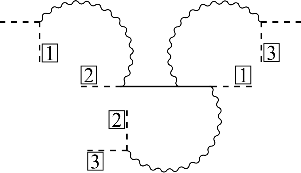
Here we prove that frequency integrations are UV finite in the limit. In this limit, the fermion Green’s function in Eq. (18) becomes . At first, it appears dangerous to take the limit because the fermion propagator is not suppressed at large frequencies. It turns out that this does not cause any UV divergence because all internal frequencies in a given diagram are bounded by the external frequencies. To begin with the proof, we note that there are different ways to label internal frequencies for a given diagram. As an example, we show two different ways of assigning internal frequencies within a three-loop fermion self-energy diagram in Figs. 11 and 11. It turns out that there is a special choice which is more convenient for our proof. This is the choice where each loop (denoted by the dotted lines in Fig. 11) associated with an internal frequency contains at least one fermion propagator which does not belong to other loops. We call this choice an ‘exclusive loop covering’. Fig. 11 is not an exclusive loop covering because the loop for does not have any ‘exclusive’ fermion propagator which carries only . On the other hand, Fig. 11 is an exclusive loop covering because for every there is at least one exclusive fermion propagator which carries only . The exclusive fermion propagator for each internal frequency is denoted as dashed lines in Fig. 11.
Does an exclusive loop covering exist for every diagram ? To show that the answer is yes, we note that any diagram can be constructed out of a connected tree diagram by contracting some of its legs. This is always possible because one can keep cutting internal lines until all loops disappear without cutting the diagram into two disconnected ones. For example, the three-loop fermion self-energy diagram in Fig. 11 is constructed by joining three pairs of legs in the tree diagram shown in Fig. 11. In Fig. 11, we represent the internal lines of the parent tree diagram by solid lines and the new internal lines created through the joining procedure by dashed lines. A loop is formed by contracting a pair of legs, where an internal frequency is assigned to run through solid lines and the dashed line created from a new contraction. For each loop formed in this way, the solid propagators are in general shared by multiple loops while each of the dashed propagators, i.e. the ones formed by contracting external legs of the tree graph, are exclusive to one loop. Since this is true for all loops, we obtain an exclusive loop covering for the diagram.

Now we show that every internal frequency is bounded by the external frequency using the exclusive loop covering. As a simple example, let us examine the three-loop fermion self-energy diagram more closely. Each internal line carries a linear combination of the external frequency and internal frequencies as is shown in Fig. 12. The key reason for the existence of an upper bound for internal frequencies is chirality. Since the fermions are chiral, the fermion propagator in Eq. (18) vanishes for positive (negative) frequency with (). As a result, there is a set of constraints that internal frequencies have to satisfy for a given set of relative coordinates between vertices. For the three-loop self-energy diagram, the constraints read
| (35) | ||||
| (36) | ||||
| (37) | ||||
| (38) | ||||
| (39) |
Here is the separation between the vertices and which are labeled in Fig. 12. The constraints in Eqs. (35) - (37) are the constraints from the exclusive propagators each of which carries only one internal frequency. Let be the set of internal frequencies that satisfy Eqs. (35) - (39). Once the signs of ’s are fixed, the set does not depend on the magnitudes of ’s. Our goal is to show that the set is bounded by the external frequency in all directions in the space of internal frequencies. To see this, we first add all non-exclusive constraints that contain . In this case, they are Eqs. (38) and (39). This leads to an inequality for ,
| (40) |
Together with Eq. (35), Eq. (40) limits the range of as
| (41) |
Eqs. (36) and (41) constrain the range of as
| (42) |
Finally, Eq. (42) together with Eq. (37) leads to
| (43) |
This implies that for a fixed set of , is bounded by . Applying this to Eqs. (41) and (42), we find that and are also bounded by .
Let be the set of internal frequencies that satisfy Eqs. (41) - (43). It is of note that not only depends on the signs of ’s but also on their magnitudes unlike . An important property of is that for any . This is due to the fact that Eqs. (41) - (43) are necessary (not sufficient in general) conditions of Eqs. (35) - (39). Since is bounded for any fixed set of , is also bounded by the external frequency in all directions in the space of internal frequencies. This proves that the integration over the internal frequencies is UV finite.
This argument can be easily generalized to all other diagrams. The rule is as follows. Consider a diagram with loops with internal fermion propagators and vertices. For a fixed set of relative coordinates of the vertices, there exist constraints for internal frequencies. Since vertices are normal ordered, fermion propagators can connect only distinct vertices. The existence of an exclusive loop covering implies that for every internal frequency there exists an exclusive constraint of the form,
| (44) |
where and is the separation between the two vertices connected by the fermion propagator which carries only . Therefore the constraints can be divided into the ‘exclusive’ constraints and ‘non-exclusive’ constraints. Non-exclusive constraints in general contain external frequencies and more than one internal frequency,
| (45) |
where is a set of external frequencies and . Without loss of generality, we can assume that only the first non-exclusive constraints, contain . We add them up to create a new constraint,
| (46) |
Since the first exclusive constraint is written as
| (47) |
it is guaranteed that is of the form
| (48) |
This is due to the fact the relative coordinates of the vertices around a loop form a cyclic sum in , and it is independent of . With the aid of Eqs. (47) and (48), we see that is bounded by other internal frequencies and the external frequencies,
| (49) |
Next we construct a set of non-exclusive constraints for made of
| (50) |
Using this set of non-exclusive constraints, we apply the same procedure for . Namely, we add all non-exclusive constraints that contain to construct a new constraint . Combined with , one can obtain a bound for of the form,
| (51) |
In this way, one can show that the range of is bounded by a linear combination of the external frequencies and the internal frequencies with ,
| (52) |
The last internal frequency is bounded only by the external frequencies,
| (53) |
The set of inequalities given by Eq. (52) implies that all the internal frequencies are bounded by the external frequencies. From the argument given below Eq. (43), the set of internal frequencies that satisfy the original constraints given by Eqs. (44) and (45) are also bounded by the external frequencies. Because all internal frequencies are bounded, all frequency integrations are UV finite even in the limit. This completes the proof that integrations over internal frequencies are UV finite for general diagrams. We emphasize that the UV finiteness is due to the chiral nature of the theory. For non-chiral theories, internal frequencies are not bounded by external ones.
VI.2.2 UV finiteness of -momentum integrations
It is easier to see that -momentum integrations are UV finite. Let us first consider fermion loops which refer to loops that are solely made of fermion propagators. For example, a bubble in Fig. 13 leads to an integration of the form,
| (54) |
where is the relative coordinate between the two quartic vertices, is the -momentum that runs inside the loop, and is the -momentum transfer. It is noted that fermion propagators and the four-fermion vertices do not depend on the -momentum that runs within the fermion loop except for the phase factor that results in Eq. (54). This leads to large fluctuations in the -momentum of the internal fermion. Due to the emergent uncertainty relation between the -coordinate and -momentum, as is manifest from the phase factor , wild fluctuations in leads to a ‘confinement’ of the relative coordinate of the two vertices . In the limit, the integration over simply generates a delta function that puts a constraint on the positions of the vertices attached to the loop, which leads to after the integration over . For a fermion loop with more than two external legs, the integration over the -momentum along the fermion loop fixes one of the coordinates of the vertices without UV divergence.
Now we consider mixed loops which refer to loops that contain at least one boson propagator. One can always assign internal momenta such that every mixed loop has at least one boson propagator which carries no other internal momenta except for the one associated with the loop. This can be easily understood from an argument that is similar to the one used in the previous section to show the existence of an exclusive loop covering for fermion propagator. This time, we cut boson propagators to remove all mixed loops without creating disjoint diagrams. For each mixed loop removed from this procedure, the boson propagator that is cut is identified as the exclusive propagator. Therefore, each internal -momentum integration of the original diagram goes as
| (55) |
at most in the large limit. For this is UV convergent in the limit.
VI.3 IR finiteness
There are two reasons for the UV finiteness of the Wilsonian action. First, -dimension is below the upper critical dimension for . As a result, only a finite number of diagrams are potentially UV divergent. Second, even the potentially divergent diagrams are finite due to chirality, which strictly limits the ranges of internal frequencies by the external ones.
On the other hand, the IR finiteness in the limit is less obvious. For example, the integration over the -momentum in Eq. (55) is IR divergent for with . While the UV finiteness is controlled by kinematic constraints, the way IR finiteness is restored in the limit is through dynamical mechanism. It turns out that the theory cures the IR singularity dynamically such that the theory flows to an IR fixed point governed by the scaling in Eq. (33). In the following section, we will see that this is indeed the case through an explicit computation of the Wilsonian effective action.
VI.4 An explicit computation of the Wilsonian effective action
Because the theory flows to a strongly interacting fixed point, it is not easy to compute the full Wilsonian effective action exactly. However, one can compute the effective action in the limit the running cut-off length scale is small compared to the length scales associated with external momenta. The main outcome of the explicit calculation is that the operators that are generated from the RPA channels shown in Fig. 14 are the only ones that are in this limit. All other channels generate operators with extra factors of accompanied by additional factors of frequency or momentum. Therefore, those contributions are suppressed in the small momentum limit with fixed (equivalently small limit with fixed momenta). Once the corrections are consistently taken into account in the Wilsonian effective action, the IR singularity encountered in the limit is cured. We first illustrate the dominance of the RPA diagrams in the small limit by computing two representative diagrams, followed by a generalization to all diagrams.
VI.4.1 order

As a first example, let us consider the diagram shown in Fig. 13, where two quartic vertices are fused into one quartic vertex as two pairs of fermion fields are contracted. The one-loop contribution is given by
| (56) | ||||
| (57) |
where and is the relative coordinate between the two vertices. The singular dependence of on again signifies the importance of the local curvature of Fermi surface. The second line in Eq. (56) represents the contribution from the fermion loop. The integration over the -momentum that runs within the fermion loop results in . Due to the delta function, the non-zero contribution is concentrated at . As a result, Eq. (57) is independent of .


Similarly, the fusion of quartic vertices in the RPA channel, as is shown in Fig. 14, generates a -loops diagram which is given by
| (58) |
For the derivation of Eq. (58), see Appendix B.1. As is the case for the fusion of two vertices shown in Fig. 13, relative coordinates between vertices are completely fixed by the delta functions that result from the wildly fluctuating flavors within the fermion loops. Therefore, all operators generated from fusions in the RPA channel are independent of . The infinite series of operators that are can be summed over to renormalize the boson propagator to
| (59) |
Note that the limit of the quartic vertex is now well defined even in the limit. As a result, the IR divergence we encountered in integrations over -momentum (for example in Eq. (55)) in the limit is cured by the quantum corrections. Henceforth, we set to focus on the critical point.
There are contributions to the quadratic vertex as well. These are generated by contracting an extra pair of fermion fields in the diagrams that generate correction to the quartic vertex. Diagrammatically, these are nothing but the RPA diagrams for the fermion self-energy as is shown in Fig. 14, where the number of fermion loops matches with the number of relative coordinate between vertices. The correction to the quadratic action is given by
| (60) |
where the self-energy is
| (61) |
with
| (62) |
It is noted that the integration over the -momentum (represented by ) in Eq. (62) is finite with because the IR divergence is cured by the series of RPA diagrams. We emphasize that the RPA diagrams are dynamically selected, not by hand. As will be shown in the following section, all other diagrams vanishes at least linearly in in the small limit due to the chiral nature of the theory. Those contributions necessarily contain larger powers of momentum or frequency, which are suppressed at low momentum/frequency.
VI.4.2 Higher order in


To illustrate the generic feature of operators generated from fusion in non-RPA channels, we compute the two-loop vertex correction shown in Fig. 15. Here three quartic operators are fused into one quartic vertex, which results in
| (63) |
where and are the two relative coordinates of the three vertices integrated over the region of -space, with defined in Eq. (151). The -momentum running in the fermion loop generates , which fixes one of the relative coordinates (). The integration over the other relative coordinate () gives rise to a factor of . Since the remaining internal momentum and frequency integrals are UV finite, the resulting operator vanishes linearly in the limit,
| (64) |
where is proportional to . The expression becomes simpler when one of the frequencies vanishes,
| (65) |
Although the integration over in the above expression is IR divergent in the limit, the divergence disappears once other operators which are also are consistently included. The other diagrams which are are the ones where the vertices and the fermion propagators in Fig. 15 are dressed by the RPA diagrams as is shown in Fig. 15. Including all the contributions amounts to replacing the bare vertices and the bare propagators in Eq. (63) with the dressed ones shown in Eqs. (59) and (61). Taking this into account, we obtain a finite expression,
| (66) |
where is a finite universal function which has the following asymptotic behavior,
| (67) | ||||
| (68) |
It is noted that the non-RPA correction is suppressed by an extra factor of in the small limit with fixed .
VI.4.3 General arguments
In this section we provide a general argument for the statement that all non-RPA diagrams contain positive powers of in the small limit. Consider a cluster of vertices which are to be fused into one vertex through a fusion channel with fermion loops. They have relative coordinates to be integrated over the range which is order of . Integrating out the -momenta running in these loops yields -functions for the relative coordinates, . After relative coordinates are fixed, the remaining relative coordinates give rise to a factor of . This implies that the only contributions are the diagrams with . These are exactly the RPA diagrams. All other diagrams, including higher order vertices generated from the quartic vertex, necessarily include positive powers of .
If the Wilsonian effective action were UV divergent in the limit, then should be kept finite. In such a case, the extra power of in the non-RPA diagrams could be saturated by or . In the present theory, there is no UV divergence due to chirality and . As a result, one can take the limit. Since there is no scale in the Wilsonian effective action, the extra powers of in the non-RPA diagrams should be accompanied by extra powers of momenta or frequency. This is why all non-RPA diagrams are suppressed in the low momentum/frequency limit with fixed .
VI.4.4 The Wilsonian effective action
Including the corrections to the zeroth order in , we obtain the Wilsonian effective action which is exact modulo irrelevant terms,
| (69) |
where and are positive constants. The effective action is local in the x-direction but not in the -direction as can be seen from the terms that are non-analytic in frequency. Once non-analytic terms are allowed in the effective action, usually the standard RG procedure becomes less useful because, in principle, infinitely many marginal or relevant non-local operators are generated. In the present case, however, the chiral nature of the theory puts a strong constraint on the form of non-local terms that can be generated. The contributions from non-RPA diagrams are systematically suppressed by positive powers of , or compared to the RPA contributions that are included in Eq. (69), where and are external frequency and -momentum of the operator. Higher order vertices such as are also generated. These vertices can be obtained by cutting open some internal lines from quartic vertices. As a result, they necessarily have less constraints on the relative coordinates of the vertices compared to the RPA diagrams. Since they are accompanied by positive powers of , they are negligible in the low energy limit. Therefore, the effective action in Eq. (69) includes all terms apart from the terms that are irrelevant by power counting. It is emphasized that RPA diagrams are dynamically selected to generate the leading order terms in the Wilsonian effective action.
With the renormalized action, it is more convenient to use a new normal ordering scheme based on the dressed Green’s function,
| (70) |
The new normal ordering is related to the old one through
| (71) |
This transformation modifies only the irrelevant operators in the action because the difference in the propagator vanishes in the low energy limit,
| (72) |
From now on, all composite operators are understood to be normal ordered according to Eq. (17) with replacing .
VI.5 Wilsonian effective action vs. quantum effective action

How was it possible for us to construct the Wilsonian effective action in Eq. (69) in the strongly coupled field theory ? The answer to this question lies in the difference between the quantum effective action and the Wilsonian effective action. In the quantum effective action computed in Ref. [37], quantum fluctuations are fully incorporated, including the contributions from the gapless modes right on the Fermi surface. On the contrary, in the Wilsonian effective action constructed in Eq. (69), only the short-distance quantum fluctuations up to the length scale are included. Therefore, the diagrams that are of the same order as the RPA diagrams in the quantum effective action do not necessarily come in the same order in the Wilsonian effective action. In this section, we show that non-RPA diagrams are indeed sub-leading in the Wilsonian effective action although they are not suppressed in the full quantum effective action.
As a concrete example, we consider a three-loop diagram shown in Fig. 16, where three quartic vertices are fused into a quadratic vertex in the Wilsonian effective action. The resulting vertex is given by
| (73) |
where the self-energy is
| (74) |
The dimensionless function is
| (75) |
where is finite for all . It has the following asymptotic behaviors,
| (76) | |||||
| (77) |
We note that the exponential factor in the last line of Eq. (75) is less than . In order to obtain an upper bound in the small limit in Eq. (76), we can simply replace the exponential factor by . Since the rest of the integrals are finite, should be proportional to in the small limit. The limit in Eq. (77) follows from the observation that the function multiplying in the exponent in Eq. (75) is strictly greater than and is . Therefore, as the leading order contribution to the integral comes from the region , resulting in the asymptotic behavior in Eq. (77).

We numerically compute , and confirm the asymptotic behaviors as is shown in Fig. 17.
In the Wilsonian effective action, we consider the low energy limit with fixed . In this case, the limit in Eq. (76) applies, and the three-loop self-energy has an extra factor of compared to the leading order terms in Eq. (61). Therefore, the diagram do not contribute to the Wilsonian effective action to the leading order. In the full quantum effective action, on the other hand, we consider the limit with fixed external frequency. In this case, the limit in Eq. (77) applies, and the diagram has the same scaling behavior as the RPA contributions. In the renormalization group, only short distance quantum fluctuations are included in every step of coarse graining. In combination with the chiral nature of the theory which constrains the degree of UV/IR singularity of the theory, this allows one to compute the exact Wilsonian effective action to the leading order.
Having said that the Wilsonian effective action can be computed perturbatively in the low momentum/frequency limit with fixed , we note that physical observables are given by the full quantum effective action. If one wants to compute physical observables with external -momenta using the effective action defined at a scale with , one still has to include the quantum fluctuations between scales and , which are not included in the Wilsonian effective action. Therefore, the exact form of the -point function, which is not dictated by the scaling, in general can not be computed perturbatively.
VII Renormalization group


It is now straightforward to perform the renormalization group analysis by increasing by a factor of in the Wilsonian effective action. The quantum correction obtained by increasing can be easily read from
| (78) |
where is the effective action in Eq. (69). The key observation is that is independent of apart from irrelevant terms. This implies that there is no quantum correction to the leading order terms in the Wilsonian effective action.
Here we show that there is indeed no quantum corrections to the leading order through an explicit calculation. We divide the configuration space of operators into two parts. The first part represents the configurations where no two composite operators are closer than along the -direction for an infinitesimally small . The second part represents the configurations where there is at least one pair of operators whose separation along the -direction is in
| (79) |
Two operators whose relative separation is in are fused into one composite operator. The volume of the phase space where more than two operators fuse simultaneously is at most order of , which can be ignored.
Now we compute the quantum corrections explicitly. Fig. 18 shows the channels where two quartic operators fuse into quadratic or quartic operators. The fusions generate the following vertices,
| (80) | ||||
| (81) | ||||
| (82) | ||||
| (83) | ||||
| (84) | ||||
| (85) | ||||
where and . Here we suppress the reference to the coordinate in to simplify the notation. The universal crossover functions, ’s, are given by
| (86) | ||||
| (87) | ||||
| (88) | ||||
| (89) | ||||
The absence of quantum corrections in Eqs. (80) and (82) is a consequence of the fact that the RPA diagrams are independent of . All non-vanishing quantum corrections are proportional to . Moreover, crossover functions are finite for . From dimensional ground, this implies that all quantum corrections come with an additional factor of momentum or frequency. Therefore all quantum corrections in Fig. 18 are irrelevant relative to the terms that are already present in the effective action.
The scaling is easily determined from the scaling that leaves the Wilsonian effective action in Eq. (69) invariant. In order to put the cut-off structure to the original form after the coarse graining, we re-scale frequency, -coordinate, -momentum and the field as
| (90) | |||||
| (91) | |||||
| (92) | |||||
| (93) |
The dynamical critical exponent , the scaling dimension of the fermion field , and the dimension of -momentum should be determined from the condition that the action is invariant. The condition that the marginal term should be scale invariant fixes the scaling dimension of the field to be
| (94) |
Then the beta functions for , , and are given by
| (95) | |||
| (96) | |||
| (97) | |||
| (98) |
One can find a fixed point for the beta functions if and only if we choose
| (99) | |||||
| (100) |
This uniquely fixes the dynamical critical exponent and the scaling dimension of the field.

One can check that higher order vertices that are generated from the quartic vertices are all irrelevant under the scaling in Eqs. (90) - (93). As an example, we compute the quantum correction where two quartic vertices fuse into a sixth order vertex as is shown in Fig. 19. In the small limit, it becomes
| (101) |
According to the scaling in Eq. (100) and the expression of in Eq. (94), this is irrelevant. This can be readily seen from the fact that the prefactor is proportional to which has scaling dimension . This is true for any higher order vertices generated during the RG flow. Contributions from these higher order vertices to the quadratic and quartic vertices are also irrelevant.
As expected, the scaling form in the chiral non-Fermi liquid state is fixed by the scaling in Eq. (33) where the interaction is kept invariant while the frequency dependent term in the bare quadratic action is deemed strongly irrelevant. This implies that the theory flows to a strongly interacting non-Fermi liquid fixed point in the low energy limit. It is remarkable that it is possible to obtain the exact scaling relation for the strongly interacting non-Fermi liquid fixed points. The scaling relation in Eq. (100) suggests that the exact fermion Green’s function in the momentum space has the form,
| (102) |
where and is a universal function. Note that the one-loop Green’s function obeys the scaling form in Eq. (102). In other words, chirality allows us to extract the scaling form of the exact Green’s function, from the one-loop Green’s function. However, the dimensionless function is not fixed by scaling, and the exact form of can be, in principle, very different from what is inferred from the one-loop Green’s function.
VIII General patch theories

The theory with the dynamical critical exponent captures the low energy physics near the Fermi surface with nonzero quadratic curvatures. There exist special points where the quadratic curvature vanishes. In particular, the periodicity of the first Brillouin zone in the direction guarantees that there exist inflection points as is shown in Fig. 20. For example, the dispersion in Eq. (3) has two inflection points at . In the neighborhood of one of the inflection points (say ), the dispersion can be written as , where is a deviation from the inflection point. Defining , , the local dispersion is written as
| (103) |
with the cubic curvature given by . Henceforth, we will drop the prime in , . With some extra fine tuning, one can even have a higher inflection points with a local dispersion,
| (104) |
with . Therefore, a general patch theory for chiral non-Fermi liquids can be parameterized by ,
Here is a positive integer greater than , and is an even integer for local theories.
VIII.1 UV finiteness and exact scaling
In this section, we show that each of the theory parameterized by in Eq. (VIII) describes a distinct and stable non-Fermi liquid fixed point for and . For , the theory should be modified by term which becomes relevant at the Gaussian fixed point. The RG analysis for general is similar to that for the theory with discussed in Secs. V - VII. In this section, we will quickly recapitulate the key results from the previous sections that apply to general , and emphasize new features that are absent in the case with . In the mixed-space of -coordinate and frequency, the action is written as
| (105) |
Again, refer to -momenta. Two comments are in order for the general theory in Eq. (105). First, the phase factor in the quartic interaction includes powers of -momenta which is inherited from the dispersion in Eq. (104). As a result, the sliding symmetry associated with is absent for . Second, the number of points with a common tangent vector determines the representation of the fermion field under the flavor group. For , the two inflection points have different tangent vectors as is shown in Fig. 20. Since the two are decoupled at low energies, only one point needs to be kept in the low energy effective theory. As a result, one does not need to double the representation as in Eq. (5).
Now we consider the Wilsonian effective action with a running cut-off scale , which is obtained by fusing operators whose separation in -direction is less than . As is the case for discussed in Sec. VI, the Wilsonian effective action is finite in the and limit. Since the integrations over internal frequencies are insensitive to the value of , one can use the exactly same argument presented in Sec. VI.2 to show that they are finite : all internal frequencies are bounded by the external frequencies due to chirality. The integrations over -momenta are also UV convergent for . As is discussed in Sec. VI.2.2, an integration over -momentum which goes through a boson propagator is UV convergent because it is suppressed as at large momentum. The only exceptions are the fermion loops which are solely made of fermion propagators. This is because the fermion propagator does not depend on -momentum, and the integration over it diverges in the absence of the phase factor which cuts off the divergence. For example, the integration over -momentum in the RPA bubble reads
| (106) |
in the limit, where is the -momentum that runs in the loop, is the momentum transferred across the loop, and is the relative coordinate between two vertices. The fact that the UV divergence from large -momenta is cut-off by a length scale in -direction is a consequence of the non-commutativity between -coordinate and -momentum as discussed in Sec. IV. Because , this gives rise to a UV enhancement factor of in the limit for every fermion loop. Although Eq. (106) is singular in the limit, it is integrable for . (For , it gives rise to a delta function for the relative coordinate.) Once the relative coordinate between vertices is integrated over, the RPA bubble is order of
| (107) |
for and a constant independent of for .
Because the Wilsonian effective action is UV finite, one can take the limit. Since there is no scale in the full quantum theory, the low energy physics should be invariant under the scale transformation which leaves the rest of the terms in Eq. (105) invariant. In other words, the Wilsonian effective action should be invariant under the coarse graining followed by a re-scaling of the field and momenta dictated by the following scaling dimensions,
| (108) | |||||
| (109) | |||||
| (110) | |||||
| (111) | |||||
| (112) | |||||
| (113) |
Eqs. (108) - (113) give the exact dynamical critical exponent and scaling dimensions.
VIII.2 The Wilsonian effective action
VIII.2.1 The RPA correction
In this section, we compute the Wilsonian effective action in the small limit. Let us estimate the magnitude of an operator generated by fusing quartic vertices in the small limit. The fusion of vertices involves relative coordinates that are integrated over the range of . This leads to a factor of . As is discussed in the previous section, each fermion loop gives rise to a UV enhancement factor of . This gives a net factor of
| (114) |
for a diagram with vertices and fermion loops. Indeed, Eq. (114) is the full answer for , as we have seen in in Sec. VI. For we will see that there are corrections to Eq. (114). To see this, we first consider the RPA diagrams which are largest in the small limit according to Eq. (114). The RPA bubble dresses the quartic vertex to (see Appendix C.1 for derivation)
| (115) |
with
| (116) |
The key difference from the case is that the RPA correction in the dressed quartic vertex vanishes in the limit for as is shown in Eq. (107). It is crucial to include the leading quantum correction to the boson self-energy to dress the quartic vertex to cure the IR singularity as we have already seen in the case. Because the IR singularity is cut off by the RPA correction, which vanishes in the small limit, each integration over -momentum that goes through a boson propagator leads to an IR enhancement factor,
| (117) |
Taking the IR enhancement factor into account, the naive power counting in Eq. (114) is modified as
| (118) |
where is the number of ‘mixed loops’ that contain at least one boson propagator in contrast to fermion loops. We use the identity , and assume that only one boson propagator becomes singular at a time within each mixed loop. Since the coefficients of and are positive for , higher loop diagrams are suppressed in the small limit. For the fermion self-energy, the leading correction arises for which is order of . See Appendix C.2 for an explicit computation of the leading correction to the quadratic action. Therefore the Wilsonian effective action with the leading order quantum corrections is written as
| (119) |
where
| (120) | ||||
| (121) |
with
| (122) |
The expression in Eq. (122) is well defined for any . Note that is complex for odd and . This appears to break the inversion along the direction under which is mapped to . However, the full theory which includes the other patch with the opposite -momentum respects the inversion as is explained in Appendix C.3.
It is noted that in the fermion self energy is singular in the limit for , which reflects the fact that the IR divergence is cut off by the quantum correction which vanishes in the limit in Eq. (115). Although diverges in the limit for , its feedback to the Wilsonian effective action is sub-leading in the small limit. This can be seen from the dressed fermion propagator,
| (123) |
Because for propagators that enter in OPE’s for the Wilsonian effective action, we have in the limit. As a result, one can ignore the exponential factor in Eq. (123) to the leading order in .
VIII.2.2 Beyond the RPA correction

Non-RPA corrections are suppressed in the small limit. For example, a non-RPA diagram with and shown in Fig. 21 contributes
| (124) |
where
| (125) | ||||
| (126) | ||||
Since the cross-over function has complicated dependence on the dimensionless parameters, let us consider a particular limit to compare with the RPA correction. We consider the small frequency limit with fixed -momenta, where , and . In this limit, the cross-over function becomes
| (127) |
resulting in the quantum correction,
| (128) |
This is smaller than the RPA dressed vertex in Eq. (119) in the limit under consideration.


There are diagrams which do not obey the counting in Eq. (118). For example, the diagram shown in Fig. 22 has a smaller power of than predicted in Eq. (118). In this diagram, there are two boson propagators (the ones outside the box in Fig. 22) which carry exactly same momentum. In the absence of the RPA correction to the quartic vertex, the two boson propagators become singular simultaneously. As a result, the integration over the -momentum that goes through the two boson propagators has a larger IR enhancement factor than predicted in Eq. (117). However, we can not consider this diagram by itself because it is part of an infinite series of diagrams as is shown in Fig. 23. The quartic vertex dressed by higher-loop boson self-energies can be written as
| (129) |
where
Here is the RPA correction defined in Eq. (175) and represents the corrections beyond the RPA level. includes the sub-diagram inside the box in Fig. 22. The one-particle irreducible non-RPA correction is suppressed compared to according to Eq. (118). Therefore, the RPA diagram dominates in the small limit.
Although, the diagram in Fig. 23 is consistent with Eq. (118), we do not have a systematic way of computing the exact dependence on for general diagrams. However, we emphasize that the scaling dimensions in Eq. (113) hold exactly irrespective of the magnitudes of individual diagrams in the small limit.
IX Thermodynamic response
One full Fermi surface generally includes multiple patch theories with different values of that belong to different universality classes. What is then the thermodynamic response of the whole system? Here we consider the case where the quadratic curvature is nonzero except for an isolated inflection point of the -th order.
Suppose there is an inflection, at which the fermion dispersion goes as . The -th curvature is scaled to be one. Let us consider a point on the Fermi surface near . Let be the difference in the -momentum between and . The local energy dispersion around includes the lower order terms as
| (130) |
where the term linear in is absorbed into a redefinition of , and the lower order curvatures go to zero near as with . Consider the free energy density per unit -momentum at temperature : is the contribution to the free energy density from a unit segment of the Fermi surface at point . The total free energy density is given by an integration over the momentum along the Fermi surface[51, 42],
| (131) |
where is a UV cut-off set by the size of the Fermi surface. Eq. (131) is a consequence of the fact that the -momentum has a positive scaling dimension and the theory is local in the momentum space[50]. The scaling at the inflection point, , fixes the form of the free energy density to be
| (132) |
Here we use the fact that the lower order curvatures ’s are relevant perturbations with the scaling dimension to the inflection point which is described by the theory with the dynamical critical exponent . is a universal function that describes the crossover from the high temperature scaling controlled by the inflection point to the low temperature scaling controlled by the points with nonzero quadratic curvatures. Its asymptotic behaviors are given by
| (133) | |||||
| (134) |
Eq. (133) is determined from the fact that the scaling dimension of is at the inflection point, whereas Eq. (134) follows from the fact that in the limit with . If there was a hierarchy in the magnitudes of , there could be multiple crossovers. But, in this case, there is only one crossover from the multi-critical point dictated by dispersion to the critical point with dispersion because for all , and the quadratic term is most relevant. Upon integrating along the Fermi surface, we obtain two universal terms for the free energy density,
| (135) |
where , are constants. The term is the contribution from the extended region with non-zero quadratic curvatures whereas the term is from the region near the inflection point. Therefore the specific heat scales as
| (136) |
where the first term dominates in the low temperature limit. In the presence of the most generic inflection point with for the quadratic dispersion of boson with , the specific heat of the whole system goes as
| (137) |
This analysis can be extended to other physical responses.
X Summary and discussions
In this paper we considered a class of non-Fermi liquid states without time-reversal and parity symmetries in dimensions. The chiral non-Fermi liquid states can be potentially realized at quantum critical points where two dimensional chiral Fermi surface is coupled with a critical boson associated with a spontaneous symmetry breaking. Chiral Fermi surface naturally arises on a stack of quantum Hall layers[45] or on the surface of three dimensional Weyl metals[52, 53, 54, 55]. The former example, however, is simpler because there are no gapless bulk degrees of freedom. In principle, chiral metals with multiple flavors can be realized by one stack of quantum Hall layers with . Alternatively, multiple chiral modes can arise at a junction of semiconductors with oppositely charged carriers in a uniform magnetic field.
In two-dimensional non-Fermi liquid states, the local patch description is valid due to the emergent locality in the momentum space[50]. General patch theories for the chiral non-Fermi liquid states can be classified by the local shape of the Fermi surface, the dispersion of the critical boson and the symmetry group. Although the non-Fermi liquid fixed points are described by strongly interacting quantum field theories, the stability of the fixed points can be established non-perturbatively, and the exact critical exponents can be computed. The main ingredient that makes an exact analysis possible is the chiral nature of the theory. Because of chirality, internal frequencies in scattering processes are strictly bounded by the external frequencies. Exploiting this property, it is possible to prove that the theory is UV finite below the upper critical dimension, which is the case for non-Fermi liquid states. The absence of UV divergence guarantees that the theory flows to a fixed point governed by the scaling which leaves the interaction invariant in the bare action. We also confirm the general conclusion by computing the Wilsonian effective action explicitly in the low momentum/frequency limit with a fixed running cut-off.
For the RG analysis, we formulate the low energy excitations near the Fermi surface as a collection of one dimensional fermions with a continuous flavor labelling the momentum along the Fermi surface. In this formalism, the curvature of the Fermi surface manifests itself through a non-commutative structure between a coordinate and momentum in different directions. The emergent non-commutativity leads to a UV/IR mixing in Fermi liquid states, where IR (UV) behavior of the system is sensitively controlled by UV (IR) structures. On the other hand, there is no prominent UV/IR mixing in non-Fermi liquid states due to the UV finiteness of the theory. The absence of non-trivial UV/IR mixing is what makes the patch description valid in the non-Fermi liquid states.
The chiral non-Fermi liquid states are two-dimensional cousins of the chiral Luttinger liquids in one dimension[44] whose stability is guaranteed by the absence of back scatterings. In the chiral Luttinger liquids, the scaling dimension of the fermionic operator is solely determined from the topological property of the system, independent of the microscopic details. Similarly, in the chiral non-Fermi liquids, the critical exponents only depend on the geometrical properties of the local Fermi surface and the dispersion of the critical boson. This is the reason why exact dimensions can be obtained.
Despite the similarity, the two-dimensional state can not be obtained from a finite number of coupled one-dimensional chains. This is because the low energy limit and the limit of infinite chains do not commute. The two-dimensional non-Fermi liquid state is obtained when one takes the limit of infinite chains before taking a low energy limit. This is manifest from the fact that the momentum along the Fermi surface is continuous, and it has a non-trivial scaling dimension.
XI Acknowledgment
We thank Djordje Minic, Subir Sachdev, Luiz Santos, T . Senthil, and Xiao-Gang Wen for helpful comments and discussions. The research was supported in part by the Natural Sciences and Engineering Research Council of Canada, the Early Research Award from the Ontario Ministry of Research and Innovation, and the Templeton Foundation. Research at the Perimeter Institute is supported in part by the Government of Canada through Industry Canada, and by the Province of Ontario through the Ministry of Research and Information.
XII Appendix
Appendix A UV/IR mixing
In this appendix we compute the one-loop vertex function shown in Fig. 4. In this section, we focus on the critical point with . The one-loop vertex correction describes a process where a boson with creates a virtual particle-hole pair at and , which then scatter into the final state of a particle-hole pair with and . For convenience, we assume that and the outgoing fermion is also on the Fermi surface, that is, . Then the resulting vertex function is a function of and . In order to examine the interplay between UV and IR scales, we assume that the largest momentum along the Fermi surface is given by a finite UV cut-off . As we will see below, the Fermi liquid states with and the non-Fermi liquid states with show distinct behaviour in terms of UV/IR mixing. In this appendix, we will use the conventional energy-momentum space representation.
First we consider the Fermi liquids with . We assume that the Yukawa coupling is small and use the one-loop dressed propagators given by
| (138) |
where are constants. The one-loop vertex correction with and is given by
| (139) |
where the cross-over function is
| (140) |
with
| (141) |
Here and correspond to the UV cut-off and the external -momentum scaled by the energy.
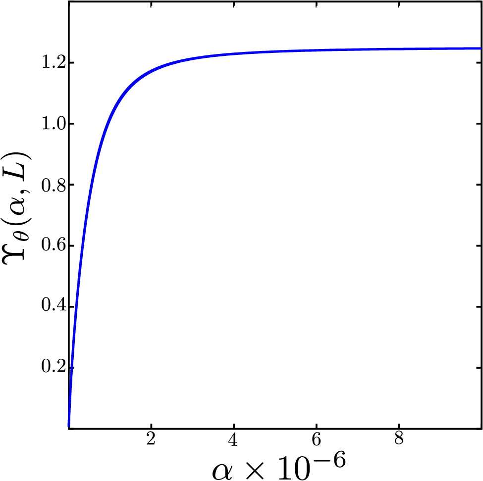
Now we examine the behavior of the vertex function as a function of . Suppose that and are fixed such that . A typical shape of the cross-over function is shown in Fig. 24 for a fixed value of . In the large limit with , the vertex correction vanishes as
| (142) |
As decreases, grows. For an intermediate regime with , the vertex correction becomes
| (143) |
As decreases, the vertex function tends to diverge as the number of virtual particle-hole pairs that can be excited within the energy provided by the boson increases. When the energy of the boson is , the range of that the virtual particle and hole can take in the loop is given by as is shown in Fig. 5. This follows from the condition . The volume of the phase space for the virtual excitations increases as decreases. However, is eventually bounded by in the presence of the UV cut-off, and the vertex function saturates to a constant as
| (144) |
in the small limit with . In other words, the maximum value of -momentum that virtual particles can have is determined by the condition,
| (145) |
For , the phase space of the virtual particle-hole excitations is controlled by the external momentum . In the opposite limit, the UV-cut off bounds the phase space. The two limits are illustrated in Fig. 5. From Eq. (145), it is evident that and limits do not commute.
It is interesting to note that the IR singularity that is present in Eq. (143) is eventually cut-off by an IR scale which is set by the inverse of the UV cut-off . This is a manifestation of UV/IR mixing where the IR behavior of the vertex function depends on the UV structure in a singular manner. The UV/IR mixing can be understood from a different perspective. For fixed , the vertex function tends to diverges as increases as far as as is shown in Eq. (144). However, the UV divergence is cut-off by a scale which is set by the inverse of the IR scale . This non-trivial interplay between UV and IR scales is a consequence of the fact that the low energy fermions near ‘feel’ the presence of other modes which carry large momenta. This situation commonly arises in quantum field theories above the upper critical dimensions. What is peculiar about the present case is that modes with large momenta are not necessarily high energy modes because gapless modes on the Fermi surface can carry large momenta. Therefore the modes at large momenta affect the low energy behaviour in a singular way. This is the origin of the UV/IR mixing.
In the Fermi liquids, the UV/IR mixing is driven by the UV sensitive volume of the phase space for low energy particle-hole excitation available near the Fermi surface. In the non-Fermi liquid state with , on the other hand, the couplings that are non-local in momentum space are suppressed. This is due to the fact that the energy of boson increases steeply at large momentum. As a result, the intermediate states of particle-hole pairs with large momenta get dynamically suppressed although those states are equally available as in Fermi liquids. This makes the vertex correction to be insensitive to the virtual processes occurring at large momenta. Therefore the UV cut-off is not important to the low energy processes for . To see this explicitly, we use the one-loop dressed fermion propagator,
| (146) |
to compute the vertex correction,
| (147) |
with
| (148) |
and is as defined in Eq. (141). In Eq. (147), the integration is convergent in the large limit even when unlike the case in Fermi liquids. For , the vertex function saturates to a constant
| (149) |
independent of the ratio in contrast to the non-trivial crossover that is present in Fermi liquid state. In this case there is no UV/IR mixing in the vertex function. The insensitivity of the physics near to the gapless modes at large momenta is the reason for the emergent locality in the momentum space[50]. As a result, one can use the patch description in non-Fermi liquid states. On the contrary, all low energy modes remain coupled with each other in the Fermi liquid state, and one has to keep the entire Fermi surface in the low energy description. Landau Fermi liquid theory indeed includes Landau parameters associated with the forward scattering across the entire Fermi surface as the low energy data.
Appendix B The RPA correction for the parabolic Fermi surface
In this section we compute the RPA vertex correction, the RPA self-energy, and derive the expressions for and in Eq. (57) and Eq. (62), respectively.
B.1 RPA vertex correction
The four-fermion vertex correction generated from the -loop RPA diagram shown in Fig. 14 is written as
| (150) |
Here is the coordinate of the -th vertex in the chain of RPA bubbles and . represents non-overlapping sets of configurations of the -coordinates of the vertices whose separations from their neighboring vertices are less than . For example, when there are three vertices at , and , there exist six distinct sets of configurations given by
| (151) |
In the present case, only two out of the sets contribute to the diagram due to the chiral nature of the theory. To see this, we first deduce the constraints on the relative coordinates of the vertices. From the -functions in the propagators, we have
| (152) |
These inequalities not only put a bound on the internal frequencies , but also impose constraints on relative coordinates : for any pair with , and are strictly ordered depending on the sign of , i.e.
- •
for ,
- •
for .
The implication of the strict ordering is that for a fixed all possess the same sign and . The integration over each leads to a -function whose support is localized in the neighborhood of . The width of the -function goes to zero in the limit the UV cutoff of ’s is sent to . As a result, the RPA diagram generates a vertex which is ultra-local in the -direction,
| (153) |
where
| (154) |
with
| (155) | ||||
| (156) | ||||
| (157) |
and
| (158) |
It is noted that the dependence of on drops out as is absorbed into the in Eq. (154).
B.2 RPA self-energy
The quantum correction generated from the -loop RPA diagrams shown in Fig. 14 is
| (159) |
where
| (160) |
with
| (161) | ||||
| (162) |
The product of the ’s in Eq. (160) yields
| (163) |
where is defined in Eq. (21). Before integrating over -momentum in Eq. (162), we use the constraints imposed by the -functions in Eq. (160) to write
| (164) |
Now we integrate over and use the property
| (165) |
along with results in Eqs. (162), (163) and (164) to obtain
| (166) |
The net contribution to the quadratic term from all RPA diagrams can be written as
| (167) |
where the RPA self-energy is
| (168) |
Here is the Fock term in Eq. (20). After summing over all loops in Eq. (168) we obtain
| (169) |
where is given by Eq. (59) and
| (170) |
for . As expected, the quantum corrections removes the spurious IR singularity at .
Appendix C The RPA correction for general shapes of the local Fermi surface
In this section we compute the RPA correction to the Wilsonian effective action for the patch theory with a general shape of the local Fermi surface.
C.1 RPA vertex correction
The four-fermion vertex correction generated from the -loop RPA diagrams shown in Fig. 14 is
| (171) |
where in the last line we have Taylor expanded the local operator around . We first compute the leading order term in the Taylor expansion which renormalizes the marginal four-fermion vertex in the action (Eq. (105)). Later we will comment on the sub-leading terms in the Taylor expansion.
C.1.1 The leading order term
The leading contribution to the four-fermion vertex from the -loop RPA diagram is
| (172) |
where
| (173) |
Due to chirality, as discussed in Appendix B, the -coordinates are strictly ordered. Hence, Eq. (173) factorizes as
| (174) |
where
| (175) |
Unlike the case with , in Eq. (175) for general depends not only on but also on one of the external -momentum because can not be absorbed by in Eq. (175). This is due to the fact that the inflection point breaks the sliding symmetry along the Fermi surface. By scaling
| (176) |
we rewrite Eq. (175) as
| (177) |
where
| (178) |
We can further simplify Eq. (178) by appealing to the parity of the integer . For even , we have
| (179) |
and for odd ,
| (180) |
To the leading order in , takes the form,
| (181) |
where was defined in Eq. (122). The dimensionless function as and is regular in the limit. Therefore, to the leading order in , and ,
| (182) |
It is of note that is independent of to the leading order in .
The infinite series of the RPA diagrams combined with the bare four-fermion vertex,
| (183) |
gives the renormalized four-fermion vertex,
| (184) |
where
| (185) |
with
| (186) |
C.1.2 The sub-leading terms
Now we consider the sub-leading terms with in Eq. (171). As we discussed in the main text, for all the relative coordinates between vertices in the RPA diagrams are fixed by the -functions arising from the fermion loops. As a result, the terms with in Eq. (171) are absent for . For the fermion loops do not produce -functions. Consequently, one has to consider the full gradient expansion in Eq. (171). In this section, we show that the gradient expansion is well defined when external momenta are small with fixed . This is less trivial than it naively looks because the two vertices at the end of the -loop RPA chains can be as far as . Since can be arbitrarily large, one has to show that the contribution from large is small.
The coefficient of the derivative term, in Eq. (171) is at most
| (187) |
where are small dimensionless parameter associated with external momentum or frequency ( ) measured in the unit of ( refers to -momentum). Here we used the fact that and the fact that each fermion loop contributes a factor of . The question is how behaves in the large and limit with a fixed value of .
From Eq. (187) it is obvious that at fixed , is exponentially suppressed as a function of because of the exponential suppression in . In order to understand the behaviour of in the large limit, we consider the logarithm of ,
| (188) | ||||
| (189) |
Since and is bounded from below, the expression within the square bracket in Eq. (189) is positive definite for any . Consequently, is exponentially suppressed as a function of when . This shows that both in the large and large limits . Therefore, the derivative terms with in the Taylor expansion in Eq. (171) are suppressed compared to the leading term at low momentum/frequency limit with fixed .
C.2 RPA self-energy
Here we compute the contributions of the RPA diagrams to the quadratic action. The procedure is identical to the one used in Appendix B.2.
The self-energy generated from the -loop RPA diagrams is
| (190) |
where
| (191) |
Note that Eq. (190) is the leading term in the gradient expansion. The terms with derivatives are dropped because they are irrelevant at low momentum as discussed in Appendix C.1.2. Integrating over in Eq. (191), and using the constraints imposed by the -functions in Eq. (191), we obtain
| (192) | ||||
| (193) |
where
| (194) |
Note that differs from defined in Eq. (175) because of the different frequency dependence of the exponential damping factor.
We write the contribution from the Fock diagram in Eq. (20), which is valid for all , as
| (195) |
To the Fock diagram we add the contributions from to to obtain the RPA self-energy,
| (196) |
where
| (197) |
As in the case of in Eq. (181), to the leading order in , we have
| (198) |
Accordingly, the renormalized vertex becomes
| (199) |
to the leading order. Using Eq. (199) in Eq. (196), we obtain the leading order contribution to the self-energy,
| (200) | ||||
| (201) |
Here is a constant given by
| (202) |
Note that depends on through . Since , we have
| (203) |
C.3 Inversion symmetry along the -direction in the patch description

In this section we show that the theory of the full Fermi surface respects the inversion symmetry along the -direction as it should be although a single patch theory breaks the symmetry for odd . The effective action for even in Eq. (119) is manifestly invariant under reversing -momenta : , . For odd , the symmetry is less obvious because the four-fermion vertex includes an imaginary components in which is odd under transformation as is shown in Eq. (122). In order to see the symmetry of the full theory, one has to include the other patch connected by the inversion. This is necessary even though the two patches are in general decoupled at low energies because they have different tangent vectors.
The inversion symmetry of the full Fermi surface guarantees that the inflection points with odd arise in pairs. For example, there is a pair of inflection points with in generic chiral Fermi surfaces as is shown in Fig. 25. Suppose that the local dispersions near a pair of such inflection points are given by
| (204) |
where measures the deviation of momenta away from the inflection points, and , where . The fermion field in each local patch is related to the original field through
| (205) |
where we assume that the inflection points are at . Under the inversion of -component of momentum, the original field transforms as
| (206) |
Therefore, the inversion exchanges and as
| (207) |
In the mixed-space representation, the effective action for the two patches is given by
| (208) |
where
| (209) | ||||
| (210) |
with
| (211) |
It is now easy to check that is invariant under inversion of -component of momenta because
| (212) |
References
- [1] L. Landau, Sov. Phys. JETP 3, 920 (1957).
- [2] J. Polchinski, arXiv:hep-th/9210046v2.
- [3] R. Shankar, Rev. Mod. Phys. 66, 129 (1994).
- [4] T. Holstein, R. E. Norton, and P. Pincus, Phys. Rev. B 8, 2649 (1973).
- [5] M. Y. Reizer, Phys. Rev. B 40, 11571 (1989).
- [6] P. A. Lee, Phys. Rev. Lett. 63, 680 (1989).
- [7] P. A. Lee and N. Nagaosa, Phys. Rev. B 46, 5621 (1992).
- [8] B. I. Halperin, P. A. Lee, and N. Read, Phys. Rev. B 47, 7312 (1993).
- [9] B. L. Altshuler, L. B. Ioffe and A. J. Millis, Phys. Rev. B 50, 14048 (1994).
- [10] J. Polchinski, Nucl. Phys. B 422, 617 (1994).
- [11] Y. B. Kim, A. Furusaki, X.-G. Wen and P. A. Lee, Phys. Rev. B 50, 17917 (1994)
- [12] Ar. Abanov and A. V. Chubukov, Phys. Rev. Lett. 84, 5608 (2000); Phys. Rev. Lett. 93, 255702 (2004).
- [13] O. I. Motrunich and M. P. A. Fisher, Phys. Rev. B 75, 235116 (2007).
- [14] H. v. Lohneysen, A. Rosch, M. Vojta and P. Wol e, Rev. Mod. Phys. 79, 1015 (2007)
- [15] P. Coleman, Heavy Fermions: electrons at the edge of magnetism, in the Handbook of Magnetism and Advanced Magnetic Materials. Edited by Helmut Kronmuller and Stuart Parkin. Vol 1: Fundamentals and Theory. John Wiley and Sons, 95-148 (2007).
- [16] T. Senthil, Phys. Rev. B 78, 045109 (2008).
- [17] D. Podolsky, A. Paramekanti, Y. B. Kim, and T. Senthil, Phys. Rev. Lett. 102, 186401 (2009).
- [18] V. Oganesyan, S. A. Kivelson, and E. Fradkin, Phys. Rev. B 64, 195109 (2001).
- [19] W. Metzner, D. Rohe, and S. Andergassen, Phys. Rev. Lett. 91, 066402 (2003);
- [20] L. Dell’Anna and W. Metzner, Phys. Rev. B 73, 045127 (2006); Phys. Rev. Lett. 98, 136402 (2007).
- [21] H.-Y. Kee, E. H. Kim, and C.-H. Chung, Phys. Rev. B 68, 245109 (2003).
- [22] M. J. Lawler, V. Fernandez, D. G. Barci, E. Fradkin, and L. Oxman, Phys. Rev. B 73, 085101 (2006); M. J. Lawler and E. Fradkin, Phys. Rev. B 75, 033304 (2007).
- [23] J. Rech, C. Pepin, and A. V. Chubukov, Phys. Rev. B 74, 195126 (2006).
- [24] P. Wolfe and A. Rosch, J. Low Temp. Phys. 147, 165 (2007).
- [25] D.L. Maslov and A.V. Chubukov, Phys. Rev. B 81, 045110 (2010).
- [26] J. Quintanilla and A. J. Schofield, Phys. Rev. B 74, 115126.
- [27] H. Yamase and H. Kohno, J. Phys. Soc. Jpn. 69, 2151 (2000).
- [28] H. Yamase, V.Oganesyan, and W. Metzner, Phys. Rev. B 72, 35114 (2005).
- [29] C. J. Halboth and W. Metzner, Phys. Rev. Lett. 85, 5162 (2000).
- [30] P. Jakubczyk, P. Strack, A. A. Katanin, and W. Metzner, Phys. Rev. B 77, 195120 (2008).
- [31] M. Zacharias, P. Wölfe, and M. Garst, Phys. Rev. B 80, 165116 (2009).
- [32] E.-A. Kim, M. J. Lawler, P. Oreto, S. Sachdev, E. Fradkin, and S. A. Kivelson, Phys. Rev. B 77, 184514 (2008).
- [33] Y. Huh and S. Sachdev, Phys. Rev. B 78, 064512 (2008).
- [34] O. I. Motrunich, Phys. Rev. B 72, 045105 (2005).
- [35] S.-S. Lee and P. A. Lee, Phys. Rev. Lett. 95, 036403 (2005).
- [36] P. A. Lee, N. Nagaosa and X.-G. Wen, Rev. Mod. Phys. 78, 17 (2006); references there-in.
- [37] S.-S. Lee, Phys. Rev. B 80, 165102(2009).
- [38] M. Metlitski and S. Sachdev, Phys. Rev. B 82, 075127 (2010); Phys. Rev. B 82, 075128 (2010).
- [39] H.-C. Jiang, M. S. Block, R. V. Mishmash, J. R. Garrison, D. N. Sheng, O. I. Motrunich, M. P. A. Fisher, Nature 493, 39 (2013).
- [40] C. Nayak and F. Wilczek, Nucl. Phys. B 430, 534 (1994).
- [41] D. F. Mross, J. McGreevy, H. Liu, and T. Senthil, Phys. Rev. B 82, 045121 (2010).
- [42] D. Dalidovich and S.-S. Lee, arxiv:1307.3170.
- [43] A. L. Fitzpatrick, S. Kachru, J. Kaplan and S. Raghu, Phys. Rev. B 88, 125116 (2013).
- [44] X.-G. Wen, Phys. Rev. B 41, 12838 (1990).
- [45] L. Balents and M.P.A. Fisher, Phys. Rev. Lett. 76, 2782 (1996).
- [46] For example, see M. R. Douglas and N. A. Nekrasov, Rev. Mod. Phys. 73, 977 (2001); R. J. Szabo, Phys. Rept. 378, 207 (2003).
- [47] S. Minwalla, M. V. Raamsdonk, and N. Seiberg, Journal of High Energy Physics 02, 020 (2000).
- [48] J. Polchinski, String Theory, Vol. 1, Cambridge University Press (1998).
- [49] J. Cardy, Scaling and Renormalization in Statistical Physics (Cambridge University Press, Cambridge, 1996).
- [50] S.-S. Lee, Phys. Rev. B 78, 085129 (2008).
- [51] T. Senthil, Phys. Rev. B 78, 035103 (2008).
- [52] F. R. Klinkhamer and G. E. Volovik, Int. J. Mod. Phys. A 20, 2795 (2005).
- [53] X. Wan, A. M Turner, A. Vishwanath, S. Y. Savrasov, Phys. Rev. B, 83, 205101 (2011).
- [54] K.-Y. Yang, Y.-M. Lu, and Y. Ran, Phys. Rev. B 84, 075129 (2011).
- [55] A. Burkov and L. Balents, Phys. Rev. Lett. 107, 127205 (2011).