Randomized LU Decomposition

Gil Shabat Address: School of Electrical Engineering, Tel Aviv University, Tel Aviv 69978, Israel Yaniv Shmueli Address: School of Computer Sciene, Tel Aviv University, Tel Aviv 69978, Israel Yariv Aizenbud Address: Department of Applied Mathematics, School of Mathematical Sciences, Tel Aviv University, Tel Aviv 69978, Israel Amir Averbuch Email: amir@math.tau.ac.il Address: School of Computer Sciene, Tel Aviv University, Tel Aviv 69978, Israel Corresponding author: Amir Averbuch, Tel: +972-54-5694455, Fax: +972-3-6422020

Abstract

Randomized algorithms play a central role in low rank approximations of large matrices. In this paper, the scheme of the randomized SVD is extended to a randomized LU algorithm. Several error bounds are introduced, that are based on recent results from random matrix theory related to subgassian matrices. The bounds also improve the existing bounds of already known randomized algorithm for low rank approximation. The algorithm is fully parallelized and thus can utilize efficiently GPUs without any CPU-GPU data transfer. Numerical examples, which illustrate the performance of the algorithm and compare it to other decomposition methods, are presented.

Keywords:

LU decomposition , matrix factorizations , random matrices , randomized algorithms

1 Introduction

Matrix factorizations and their relations to low rank approximations play a major role in many of today’s applications [41]. In mathematics, matrix decompositions are used for low rank matrix approximations that often reveal interesting properties in a matrix. Matrix decompositions are used for example in solving linear equations and in finding least squares solutions. In engineering, matrix decompositions are used in computer vision [19], machine learning [33], collaborative filtering and Big Data analytics [26]. As the size of the data grows exponentially, feasible methods for the analysis of large datasets has gained an increasing interest. Such an analysis can involve a factorization step of the input data given as a large sample-by-feature matrix or given by a sample affinity matrix [45, 12, 39]. High memory consumption and the computational complexity of the factorization step are two main reasons for the difficulties in analyzing huge data structures. Recently, there is an on-going interest in applying mathematical tools that are based on randomization to overcome these difficulties.

Some of the randomized algorithms use random projections that project the matrix to a set of random vectors. Formally, given a matrix $A$ of size $m\times n$ (assume $m\geq n$ ) and a random matrix $G$ of size $n\times k$ , then the product $AG$ is computed to obtain a smaller matrix that potentially captures most of the range of $A$ . In most of these applications, $k$ is set to be much smaller than $n$ to obtain a compact approximation for $A$ .

In this paper, we develop a randomized version of the LU decomposition. Given an $m\times n$ matrix $A$ , we seek a lower triangular $m\times k$ matrix $L$ and an upper triangular $k\times n$ matrix $U$ such that

\|LU-PAQ\|_{2}=C(m,n,k)\sigma_{k+1}(A),

(1.1)

where $P$ and $Q$ are orthogonal permutation matrices, $\sigma_{k+1}(A)$ is the $k+1$ largest singular value of $A$ and $C(m,n,k)$ is a constant that depends on $m,n$ and $k$ .

The interest in a randomized LU decomposition can be motivated (computationally wise) by two important properties of the classical LU decomposition: First, it can be applied efficiently to sparse matrices with computation time that depends on the number of non-zero elements. LU decomposition with full pivoting on sparse matrices can generate large regions of zeros in the factorized matrices [38, 15, 14]. Processing of sparse matrices will be treated in a separate paper. Second, LU decomposition can be fully parallelized [22] which makes it applicable for running on Graphics Processing Units (GPU). GPUs are mostly used for computer games, graphics and visualization such as movies and 3D display. Their powerful computation capabilities can be used for fast matrix computations [25].

The contributions of the paper are twofold: A randomized version for LU decomposition, which is based on the randomized SVD template [32, 24], is presented. The algorithm is analyzed and several error bounds are derived. The bounds are based on recent results from random matrix theory for the largest and smallest singular values of random matrices with subgaussian entries [29, 28]. This technique is also used to improve the bounds for the randomized SVD. The randomized LU is fully implemented to run on a standard GPU card without any GPU-CPU data transfer. It enables us to accelerate the algorithm significantly. We present numerical results that compare our algorithm with other decomposition methods and show that it outperforms them.

The paper is organized as follows: Section 2, overviews related work on matrix decomposition and approximation that use randomized methods. Section 3 reviews several mathematical results that are needed for the development of the randomized LU. Section 4 presents several randomized LU algorithms and several error bounds on their approximations are proved. Section 5 presents numerical results on the approximation error, the computational complexity of the algorithm and compares it with other methods. The performance comparison was done on different types of matrices and by using GPU cards.

2 Related Work

Efficient matrix decomposition serves as a basis for many studies and algorithms design for data analysis and applications. Fast randomized matrix decomposition algorithms are used for tracking objects in videos [39], multiscale extensions for data [4] and detecting anomalies in network traffic for finding cyber attacks [13], to name some. There are randomized versions for many different matrix factorization algorithms [24], compressed sensing [16] and least squares [3].

There is a variety of methods and algorithms that factorize a matrix into several matrices. Typically, the factorized terms have properties such as being triangular, orthogonal, diagonal, sparse or low rank. In general, a certain control on the desired approximation error for a factorized matrix is possible. For example, it is achievable by increasing the rank of a low rank approximation or by allowing dense factors for sparse decompositions.

Rank revealing factorization uses permutation matrices on the columns and rows of a martrix $A$ so that the factorized matrices structure have a strong rank portion and a rank deficient portion. The most known example for approximating an $m\times n$ matrix $A$ by a low rank $k$ matrix is the truncated SVD. Other rank revealing factorizations can be used to achieve low rank approximations. For example, both QR and LU factorizations have rank revealing versions such as RRQR decomposition [7], strong RRQR [23] decomposition, RRLU decomposition [35] and strong RRLU decomposition [34].

Other matrix factorization methods such as Interpolative Decomposition (ID) [9] and CUR decomposition [18], use columns and rows of the original matrix $A$ in the factorization process. Such a property exposes the most important portions that construct $A$ . An ID factorization of order $k$ of an $m\times n$ matrix $A$ consists of an $m\times k$ matrix $B$ whose columns consist of a subset of the columns of $A$ , as well as a $k\times n$ matrix $P$ , such that a subset of the columns of $P$ becomes a $k\times k$ identity matrix and $A\approx BP$ such that $\|A-BP\|\lesssim\mathcal{O}(n,\sigma_{k+1}(A))$ . Usually, $k=\#\{j:\sigma_{j}(A)\geq\delta\sigma_{1}(A)\}$ is the numerical rank of $A$ up to a certain accuracy $\delta>0$ . This selection of $k$ guarantees that the columns of $B$ constitute a well-conditioned basis for the range of $A$ [9].

Randomized version for many important algorithms have been developed in order to reduce the computational complexity by approximating the solution to a desired rank. These include SVD, QR and ID factorizations [32], CUR decomposition as a randomized version [18] of the pseudo-skeleton decomposition, methods for solving least squares problems [36, 11, 3] and low rank approximations [11, 1].

In general, randomization methods for matrix factorization have two steps: 1. A low-dimensional space, which captures most of the “energy" of $A$ , is found using randomization. 2. $A$ is projected onto the retrieved subspace and the projected matrix is factorized [24].

Several different options exist when random projection matrix is used in the step 1. For example, it can be a matrix of random signs ( $\pm 1$ ) [10, 30], a matrix of i.i.d Gaussian random variables with zero mean and unit variance [32], a matrix whose columns are selected randomly from the identity matrix with either uniform or non-uniform probability [20, 17], a random sparse matrix designed to enable fast multiplication with a sparse input matrix [11, 1], random structured matrices, which use orthogonal transforms such as discrete Fourier transform, Walsh-Hadamard transform and more ([36, 3, 6]). In our algorithm, we use Gaussian matrices in Step 1 as well as structured Fourier matrices to achieve accelerated computation.

3 Preliminaries

In this section, we review the rank revealing LU (RRLU) decomposition and bounds on singular values bounds for random matrices that will be used to prove the error bounds for the randomized LU algorithm. Throughout the paper, we use the following notation: for any matrix $A$ , $\sigma_{j}(A)$ is the $j$ th largest singular value and $\|A\|$ is the spectral norm (the largest singular value or $l_{2}$ operator norm). If $x$ is a vector then $\|x\|$ is the standard $l_{2}$ (Euclidean) norm. $A^{\dagger}$ denotes the pseudo-inverse of $A$ . For a random variable $X$ , $\mathbb{E}$ denotes the expectation of $X$ and $\mathbb{P}(X\geq x)$ is the probably of a random variable $X$ to be larger than a scalar $x$ .

3.1 Rank Revealing LU (RRLU)

The following theorem is adapted from [35] (Theorem 1.2):

Theorem 3.1 ([35]).

Let $A$ be an $m\times n$ matrix ( $m\geq n$ ). Given an integer $1\leq k<n$ , the following factorization

PAQ=\begin{pmatrix}L_{11}&0\\ L_{21}&I_{n-k}\end{pmatrix}\begin{pmatrix}U_{11}&U_{12}\\ 0&U_{22}\end{pmatrix}

(3.1)

holds where $L_{11}$ is a unit lower triangular, $U_{11}$ is an upper triangular, $P$ and $Q$ are orthogonal permutation matrices. Let $\sigma_{1}\geq\sigma_{2}\geq...\geq\sigma_{n}\geq 0$ be the singular values of $A$ , then

\sigma_{k}\geq\sigma_{min}(L_{11}U_{11})\geq\frac{\sigma_{k}}{k(n-k)+1},

(3.2)

and

\sigma_{k+1}\leq\|U_{22}\|\leq(k(n-k)+1)\sigma_{k+1}.

(3.3)

This is called RRLU decomposition. Based on Theorem 3.1, we have the following definition:

Definition 3.1 (RRLU Rank $k$ Approximation denoted RRLU_k).

Given a RRLU decomposition (Theorem 3.1) of a matrix $A$ with an integer $k$ (as in Eq. (3.1)) such that $PAQ=LU$ . The RRLU rank $k$ approximation is defined by taking $k$ columns from $L$ and $k$ rows from $U$ such that

\text{RRLU}_{k}(PAQ)=\begin{pmatrix}L_{11}\\ L_{21}\end{pmatrix}\begin{pmatrix}U_{11}U_{12}\end{pmatrix}

(3.4)

where $L_{11},L_{21},U_{11},U_{12},P$ and $Q$ are defined in Theorem 3.1.

Lemma 3.2 (RRLU Approximation Error).

The error of the RRLU_k approximation of $A$ is

\|PAQ-\text{RRLU}_{k}(PAQ)\|\leq(k(n-k)+1)\sigma_{k+1}.

(3.5)

Proof.

The proof follows directly from Eqs. (3.1) and (3.4). ∎

Lemma 3.3 appears in [5], page 75:

Lemma 3.3 ([5]).

Let $A$ and $B$ be two matrices and let $\sigma_{j}(\cdot)$ denotes the $j$ th singular value of a matrix. Then, $\sigma_{j}(AB)\leq\|A\|\sigma_{j}(B)$ and $\sigma_{j}(AB)\leq\|B\|\sigma_{j}(A)$ .

Lemma 3.4 was taken from [32] and it is an equivalent formulation for Eq. 8.8 in [21].

Lemma 3.4 ([32]).

Suppose that $G$ is a real $n\times l$ matrix whose entries are i.i.d Gaussian random variables with zero mean and unit variance and let $m$ be an integer such that $m\geq l$ , $m\geq n$ , $\gamma>1$ and

1-\frac{1}{4(\gamma^{2}-1)\sqrt{\pi m\gamma^{2}}}\left(\frac{2\gamma^{2}}{e^{\gamma^{2}-1}}\right)^{m}\geq 0.

(3.6)

Then, $\|G\|\leq\sqrt{2m}\gamma$ with probability not less than the value in Eq. (3.6).

3.2 Subgaussian Random Matrices

Definition 3.2.

A real valued random variable $X$ is called subgaussian if there exists $b>0$ such that for all $t>0$ we have $\mathbb{E}e^{tX}\leq e^{b^{2}t^{2}/2}$ .

We review several results adapted from [29, 37] about random matrices whose entries are subgaussian. We focus on the case where $A$ is a tall $m\times n$ matrix ( $m>(1+\frac{1}{\ln n})n$ ). Similar results can be found in [28] for square and almost square matrices.

Definition 3.3.

Assume that $\mu\geq 1$ , $a_{1}>0$ and $a_{2}>0$ . $\mathcal{A}(\mu,a_{1},a_{2},m,n)$ is the set of all $m\times n$ ( $m>n$ ) random matrices $A=(\xi_{ij})$ whose entries are centered i.i.d real valued random variables satisfying the following conditions:

1.

Moments: $\mathbb{E}|\xi_{ij}|^{3}\leq\mu^{3}$ ;
2.

Norm: $\mathbb{P}(\|A\|>a_{1}\sqrt{m})\leq e^{-a_{2}m}$ where $\mathbb{P}$ is a probability function;
3.

Variance: $\mathbb{E}\xi_{ij}^{2}\geq 1$ .

It is shown in [29] that if $A$ is subgaussian then $A\in\mathcal{A}$ . For a Gaussian matrix with zero mean and unit variance, $\mu=\left(\frac{4}{\sqrt{2\pi}}\right)^{\frac{1}{3}}$

Theorems 3.5 and 3.6 are taken from Section 2 in [29].

Theorem 3.5 ([29]).

Every matrix $A$ of size $m\times n$ ( $m\geq n$ ), whose entries are subgaussian with $\mu\geq 1$ and $a_{2}\geq 0$ , satisfies:

\mathbb{P}\left(\|A\|\geq a_{1}\sqrt{m}\right)\leq e^{-a_{2}m}

(3.7)

where $a_{1}=6\mu\sqrt{a_{2}+4}$ .

Theorem 3.5 provides an upper bound for the largest singular value that depends on the desired probability. Theorem 3.6 is used to bound from below the smallest singular value of random Gaussian matrices.

Theorem 3.6 ([29]).

Let $\mu\geq 1$ , $a_{1},a_{2}>0$ . Let $A$ be an $m\times n$ matrix where $m>(1+\frac{1}{\ln n})n$ . $m$ can be written as $m=(1+\delta)n$ . Suppose that the entries of $A$ are centered independent random variables such that conditions $1,2,3$ in Definition 3.3 hold. Then, there exist positive constants $c_{1}$ and $c_{2}$ such that

\mathbb{P}(\sigma_{n}(A)\leq c_{1}\sqrt{m})\leq e^{-m}+e^{-c^{\prime\prime}m/(2\mu^{6})}+e^{-a_{2}m}\leq e^{-c_{2}m}.

(3.8)

From Theorem 3.6, the exact values of constants $c_{1},c_{2}$ and $c^{\prime\prime}$ are

c_{1}=\frac{b}{e^{2}c_{3}}\left(\frac{b}{3e^{2}c_{3}a_{1}}\right)^{\frac{1}{\delta}},~~c^{\prime\prime}=\frac{27}{2^{11}}

(3.9)

where $c_{3}=4\sqrt{\frac{2}{\pi}}\left(\frac{2\mu^{9}}{a_{1}^{3}}+\sqrt{\pi}\right)$ , $b=\min\left(\frac{1}{4},\frac{c^{\prime}}{5a_{1}\mu^{3}}\right)$ and $c^{\prime}=\left(\frac{27}{2^{13}}\right)^{\frac{1}{2}}$ . For the constant $c_{2}$ , we need a small enough constant to satisfy the inequality in Eq. (3.8) and set it, for simplification, to

c_{2}=\min\left(1,\frac{c^{\prime\prime}}{(2\mu^{6})},a_{2}\right)-\frac{\ln 3}{m}.

(3.10)

The setting of $c_{2}$ according to Eq. (3.10) comes from a relaxation of the inequality

e^{-m}+e^{-c^{\prime\prime}m/(2\mu^{6})}+e^{-a_{2}m}\leq 3e^{-\min\left(1,\frac{c^{\prime\prime}}{(2\mu^{6})},a_{2}\right)}\leq e^{-c_{2}m}

and solving $3e^{-\min\left(1,\frac{c^{\prime\prime}}{(2\mu^{6})},a_{2}\right)}\leq e^{-c_{2}m}$ for $c_{2}$ .

3.3 The SRFT matrix

The Subsampled Random Fourier Transform (SRFT), which is described in [2, 46], is a random matrix $R$ with the structure $R=DFS$ where $D$ is an $n\times n$ diagonal matrix whose entries are i.i.d. random variables drawn from a uniform distribution on the unit circle in $\mathbb{C}$ , $F$ is an $n\times n$ discrete Fourier transform such that $F_{jk}=\frac{1}{\sqrt{n}}e^{-2\pi i(j-1)(k-1)/n}$ and $S$ is an $n\times l$ matrix whose entries are all zeros except for a single randomly placed 1 in each column.

Lemma 3.7 ([46]).

For any $m\times n$ matrix $A$ , let $R$ be the $n\times l$ SRFT matrix. Then, $Y=AR$ can be computed in $\mathcal{O}(mn\log l)$ floating point operations.

3.4 Interpolative decomposition (ID)

Let $A$ be an $m\times n$ of rank $r$ . $A\approx A_{(:,J)}X$ is the ID of rank $r$ of $A$ if:

1.

$J$ is a subset of $r$ indices from $1,\ldots,n$ .
2.

The $r\times n$ matrix $A_{(:,J)}$ is a subset of $J$ columns from $A$ .
3.

$X$ is an $r\times n$ matrix whose entries are less than 2 in magnitude and contains $r$ columns of the identity matrix.

Similarly, it is possible to compute the ID with row selection such that $A\approx XA_{(J,:)}$ . The ID is based on [23] and it is introduced in [32, 9, 24] for deterministic and random algorithms. It is possible to compute ID with LU instead of using QR. This can increase the reconstruction error, since RRQR has better bounds than RRLU ([23, 35]) while reducing the computational complexity since LU is faster to compute than QR ([22]).

4 Randomized LU

In this section, we present the randomized LU algorithm (Algorithm 4.1) that computes the LU rank $k$ approximation of a full matrix. In addition, we present Algorithm 4.4 that utilizes the SRFT matrix for achieving a faster processing. Error bounds are derived for each algorithm.

The algorithm begins by projecting the input matrix on a random matrix. The resulting matrix captures most of the range of the input matrix. Then, we compute a triangular basis for this matrix and project the input matrix on it. Finally, we find a second triangular basis for the projected columns and multiply it with the original basis. The product leads to a lower triangular matrix $L$ and the upper triangular matrix $U$ is obtained from the second LU factorization.

Algorithm 4.1 Randomized LU Decomposition

Input:

A

matrix of size

m\times n

to decompose,

k

desired rank,

l\geq k

number of columns to use.

Output: Matrices

P,Q,L,U

such that

\|PAQ-LU\|\leq\mathcal{O}(\sigma_{k+1}(A))

where

P

and

Q

are orthogonal permutation matrices,

L

and

U

are the lower and upper triangular matrices, respectively.

1: Create a matrix

G

of size

n\times l

whose entries are i.i.d. Gaussian random variables with zero mean and unit standard deviation.

Y\leftarrow AG

3: Apply RRLU decomposition (Theorem 3.1) to

Y

such that

PYQ_{y}=L_{y}U_{y}

4: Truncate

L_{y}

and

U_{y}

by choosing the first

k

columns and the first

k

rows, respectively, such that

L_{y}\leftarrow L_{y}(:,1:k)

and

U_{y}\leftarrow U_{y}(1:k,:)

B\leftarrow L_{y}^{\dagger}PA

6: Apply LU decomposition to

B

with column pivoting

BQ=L_{b}U_{b}

L\leftarrow L_{y}L_{b}

U\leftarrow U_{b}

Remark 4.1.

The pseudo-inverse of $L_{y}$ in step $5$ can be computed by $L_{y}^{\dagger}=(L_{y}^{T}L_{y})^{-1}L_{y}^{T}$ . This can be done efficiently when it is computed on platforms such as GPUs that can multiply matrices via parallelization. Usually, the inversion is done on a small matrix since in many cases $k\ll n$ and therefore it can be done cheaply (computationally wise) by the application of Gaussian elimination.

Remark 4.2.

In practice, it is sufficient to perform step $3$ in Algorithm 4.1 using standard LU decomposition with partial pivoting instead of applying RRLU. The cases where $U$ grows exponentially are extremely rare – see section 3.4.5 in [22, 42].

Theorem 4.3 presents an error bound for Algorithm 4.1:

Theorem 4.3.

Let $A$ be a matrix of size $m\times n$ . Then, its randomized LU decomposition produced by Algorithm 4.1 with integers $k$ and $l$ ( $l\geq k$ ) satisfies:

\|LU-PAQ\|\leq\left(2\sqrt{2nl\beta^{2}\gamma^{2}+1}+2\sqrt{2nl}\beta\gamma\left(k(n-k)+1\right)\right)\sigma_{k+1}(A),

(4.1)

with probability not less than

\xi\triangleq 1-\frac{1}{\sqrt{2\pi(l-k+1)}}\left(\frac{e}{(l-k+1)\beta}\right)^{l-k+1}-\frac{1}{4(\gamma^{2}-1)\sqrt{\pi n\gamma^{2}}}\left(\frac{2\gamma^{2}}{e^{\gamma^{2}-1}}\right)^{n},

(4.2)

where $\beta>0$ and $\gamma>1$ .

The proof of Theorem 4.3 is given in Section 4.2. To show that the success probability $\xi$ in Eq. (4.2) is sufficiently high, we present several calculated values of $\xi$ in Table 4.1. We omitted the value of $n$ from Table 4.1 since it does not affect the value of $\xi$ due to the fact that the second term in Eq. (4.2) decays fast.

Table 4.1: Calculated values for the success probability

\xi

(Eq. (4.2)). The terms

l-k

\beta

and

\gamma

appear in Eq. 4.2.

$l-k$	$\beta$	$\gamma$	$\xi$
3	5	5	$1-6.8\times 10^{-5}$
5	5	5	$1-9.0\times 10^{-8}$
10	5	5	$1-5.2\times 10^{-16}$
3	30	5	$1-5.2\times 10^{-8}$
5	30	5	$1-1.9\times 10^{-12}$
10	30	5	$1-1.4\times 10^{-24}$
3	30	10	$1-5.2\times 10^{-8}$
5	30	10	$1-1.9\times 10^{-12}$
10	30	10	$1-1.4\times 10^{-24}$

In Section 5, we show that in practice, Algorithm 4.1 produces comparable results to other well-known randomized factorization methods of low rank matrices such as randomized SVD and randomized ID.

4.1 Computational Complexity Analysis

To compute the number of floating points operations in Algorithm 4.1, we evaluate the complexity of each step:

Step 1:: Generating an $n\times l$ random matrix requires $\mathcal{O}(nl)$ operations.
Step 2:: Multiplying $A$ by $G$ to form $Y$ requires $l\mathcal{C}_{A}$ operations, where $\mathcal{C}_{A}$ is the complexity of applying $A$ to an $n\times 1$ column vector.
Step 3:: Partial pivoting computation of LU for $Y$ requires $\mathcal{O}(ml^{2})$ operations.
Step 4:: Selecting the first $k$ columns (we do not modify them) requires $\mathcal{O}(1)$ operations.
Step 5:: Computing the pseudo inverse of $L_{y}$ requires $\mathcal{O}(k^{2}m+k^{3}+k^{2}m)$ operations and multiplying it by $A$ requires $k\mathcal{C}_{A^{T}}$ operations. Note that $P$ is a permutation matrix that does not modify the rows of $A$ .
Step 6:: Computing the partial pivoting LU for $B$ requires $\mathcal{O}(k^{2}n)$ operations.
Step 7:: Computing $L$ requires $\mathcal{O}(k^{2}m)$ operations.
Step 8:: Computing $U$ requires $\mathcal{O}(1)$ operations.

By summing up the complexities of all the steps above, then Algorithm 4.1 necessitated

\mathcal{C}_{RandLU}=l\mathcal{C}_{A}+k\mathcal{C}_{A^{T}}+\mathcal{O}(l^{2}m+k^{3}+k^{2}n)

(4.3)

operations. Here, we used $C_{A}$ (and $C_{A^{T}}$ ) to denote the complexity from the application of $A$ (and $A^{T}$ ) to a vector, respectively. For a general $A$ , $\mathcal{C}_{A}=\mathcal{C}_{A^{T}}=\mathcal{O}(mn)$ .

4.2 Bounds for the Randomized LU (Proof of Theorem 4.3)

In this section, we prove Theorem 4.3 and provide an additional complementary bound. This is done by finding a basis to the smaller matrix $AG$ , which is achieved in practice by using RRLU. The assumptions are that $L$ is numerically stable so its pseudo-inverse can be computed accurately, there exists a matrix $U$ such that $LU$ is a good approximation to $AG$ and there exists a matrix $F$ such that $\|AGF-A\|$ is small. $L$ is always numerically stable since it has a small condition number [40].

Lemmas 4.4,4.5 and 4.6 are needed for the proof of Theorem 4.3. Lemma 4.4 states that a given basis $L$ can form a basis for the columns in $A$ by bounding the error $\|LL^{\dagger}A-A\|$ .

Lemma 4.4.

Assume that $A$ is an $m\times n$ matrix, $L$ is an $m\times k$ matrix with rank $k$ , $G$ is an $n\times l$ matrix, $l$ is an integer ( $l\geq k$ ), $U$ is a $k\times l$ matrix and $F$ is $l\times n$ ( $k\leq m$ ) matrix. Then,

\|LL^{\dagger}A-A\|\leq 2\|AGF-A\|+2\|F\|\|LU-AG\|.

(4.4)

Proof.

By using the triangular inequality we get

\|LL^{\dagger}A-A\|\leq\|LL^{\dagger}A-LL^{\dagger}AGF\|+\|LL^{\dagger}AGF-AGF\|+\|AGF-A\|.

(4.5)

Clearly, the first term can also be bounded by

\|LL^{\dagger}A-LL^{\dagger}AGF\|\leq\|LL^{\dagger}\|\|A-AGF\|\leq\|A-AGF\|.

(4.6)

The second term can be bounded by

\|LL^{\dagger}AGF-AGF\|\leq\|F\|\|LL^{\dagger}AG-AG\|.

(4.7)

In addition,

\|LL^{\dagger}AG-AG\|\leq\|LL^{\dagger}AG-LL^{\dagger}LU\|+\|LL^{\dagger}LU-LU\|+\|LU-AG\|.

(4.8)

Since $L^{\dagger}L=I$ , it follows that $\|LL^{\dagger}LU-LU\|=0$ and that $\|LL^{\dagger}AG-LL^{\dagger}LU\|\leq\|AG-LU\|$ . When combined with Eq. (4.8) we obtain:

\|LL^{\dagger}AG-AG\|\leq 2\|LU-AG\|.

(4.9)

By substituting Eq. (4.9) in Eq. (4.7) we get

\|LL^{\dagger}AGF-AGF\|\leq 2\|F\|\|LU-AG\|.

(4.10)

By substituting Eqs. (4.6) and (4.10) in Eq. (4.5) we get

\|LL^{\dagger}A-A\|\leq 2\|AGF-A\|+2\|F\|\|LU-AG\|.

(4.11)

∎

Lemma 4.5 appears in [32]. It uses a lower bound for the smallest singular value of a Gaussian matrix with zero mean and unit variance. This bound appears in [8].

Lemma 4.5 ([32]).

Assume that $k,l,m$ and $n$ are positive integers such that $k\leq l$ , $l\leq\min{(m,n)}$ . Assume that $A$ is a real $m\times n$ matrix, $G$ is $n\times l$ matrix whose entries are i.i.d Gaussian random variables of zero mean and unit variance, $\beta$ and $\gamma$ are real numbers, such that $\beta>0$ , $\gamma>1$ and the quantity

1-\frac{1}{\sqrt{2\pi(l-k+1)}}\left(\frac{e}{(l-k+1)\beta}\right)^{l-k+1}-\frac{1}{4(\gamma^{2}-1)\sqrt{\pi n\gamma^{2}}}\left(\frac{2\gamma^{2}}{e^{\gamma^{2}-1}}\right)^{n}

(4.12)

is non-negative. Then, there exists a real $l\times n$ matrix $F$ such that

\|AGF-A\|\leq\sqrt{2nl\beta^{2}\gamma^{2}+1}\sigma_{k+1}(A)

(4.13)

and

\|F\|\leq\sqrt{l}\beta

(4.14)

with probability not less than the value in Eq. (4.12).

Lemma 4.6 rephrases Lemma 4.5 by utilizing the bounds that appear in Section 3.2. The proof is close to the argumentation that appears in the proof of Lemma 4.5.

Lemma 4.6.

Let $A$ be a real $m\times n$ ( $m\geq n$ ) matrix. Let $G$ be a real $n\times l$ matrix whose entries are Gaussian i.i.d with zero mean and unit variance. Let $k$ and $l$ be integers such that $l<\min{(m,n)}$ and $l>\left(1+\frac{1}{\ln k}\right)k$ . We define $a_{1},a_{2},c_{1}$ and $c_{2}$ as in Theorem 3.6. Then, there exists a real matrix $F$ of size $l\times n$ such that

\|AGF-A\|\leq\sqrt{\frac{a_{1}^{2}n}{c_{1}^{2}l}+1}\sigma_{k+1}(A),

(4.15)

and

\|F\|\leq\frac{1}{c_{1}\sqrt{l}}

(4.16)

with probability not less than $1-e^{-c_{2}l}-e^{-a_{2}n}$ .

Proof.

We begin by the application of SVD to $A$ such that

A=U\Sigma V^{T},

(4.17)

where $U$ is orthogonal $m\times m$ matrix, $\Sigma$ is $m\times n$ diagonal matrix with non-negative entries and $V$ is orthogonal $n\times n$ matrix. Assume that given $V^{T}$ and $G$ , suppose that

V^{T}G=\begin{pmatrix}H\\ R\end{pmatrix},

(4.18)

where $H$ is $k\times l$ matrix and $R$ is $(n-k)\times l$ matrix. Since $G$ is a Gaussian i.i.d. matrix and $V$ is an orthogonal matrix, then $V^{T}G$ is also a Gaussian i.i.d. matrix. Therefore, $H$ is a Gaussian i.i.d. matrix. Define $F=PV^{T}$ , where $P$ is a matrix of size $l\times n$ such that $P=\begin{pmatrix}H^{\dagger}&0.\end{pmatrix}$ Therefore,

F=\begin{pmatrix}H^{\dagger}&0\end{pmatrix}V^{T}.

(4.19)

By computing $\|F\|$ using Theorem 3.6, we get

\|F\|=\|PV^{T}\|=\|H^{\dagger}\|=\|H^{T}(HH^{T})^{-1}\|=\frac{1}{\sigma_{k}(H)}\leq\frac{1}{c_{1}\sqrt{l}}

(4.20)

with probability not less than $1-e^{-c_{2}l}$ . Now, we can bound $\|AGF-A\|$ . By using Eqs. (4.17), (4.18) and (4.19) we get

AGF-A=U\Sigma\begin{pmatrix}\begin{pmatrix}H\\ R\end{pmatrix}\begin{pmatrix}H^{\dagger}&0\end{pmatrix}-I\end{pmatrix}V^{T}.

(4.21)

We define $S$ to be the $k\times k$ upper-left block of $\Sigma$ . Let $T$ to be the $(n-k)\times(n-k)$ lower-right block. Then,

\Sigma\begin{pmatrix}\begin{pmatrix}H\\ R\end{pmatrix}\begin{pmatrix}H^{\dagger}&0\end{pmatrix}-I\end{pmatrix}=\begin{pmatrix}S&0\\ 0&T\end{pmatrix}\begin{pmatrix}0&0\\ RH^{\dagger}&-I\end{pmatrix}=\begin{pmatrix}0&0\\ TRH^{\dagger}&-T\end{pmatrix}.

The norm of the last term is:

\left\|\begin{pmatrix}0&0\\ TRH^{\dagger}&-T\end{pmatrix}\right\|^{2}\leq\|TRH^{\dagger}\|^{2}+\|T\|^{2}.

(4.22)

Therefore, by using Eqs. (4.21), (4.22) and the fact that $\|T\|=\sigma_{k+1}(A)$ , we get

\|AGF-A\|\leq\sqrt{\|TRH^{\dagger}\|^{2}+\|T\|^{2}}\leq\sqrt{\|H^{\dagger}\|^{2}\|R\|^{2}+1}\sigma_{k+1}(A).

(4.23)

We also know that

\|R\|\leq\|V^{T}G\|=\|G\|\leq a_{1}\sqrt{n}

with probability not less than $1-e^{-a_{2}n}$ . Combining Eq. (4.23) with the fact that $\|H^{\dagger}\|\leq\frac{1}{c_{1}\sqrt{l}}$ and $\|R\|\leq a_{1}\sqrt{n}$ gives

\|AGF-A\|\leq\sigma_{k+1}(A)\sqrt{\frac{a_{1}^{2}n}{c_{1}^{2}l}+1}.

(4.24)

∎

Remark 4.7.

In contrast to Lemma 4.5 where $\|AGF-A\|=\mathcal{O}(\sqrt{nl})$ , Lemma 4.6 provides the bound $\|AGF-A\|=\mathcal{O}(\sqrt{\frac{n}{l}})$ that is tighter for large values of $l$ .

Remark 4.8.

The condition $l>\left(1+\frac{1}{\ln k}\right)k$ in Lemma 4.6 has to be satisfied to meet the error bounds. However, there are bounds for the case where $H$ is almost square ( $l\approx k$ ) or square ( $l=k$ ) and they are given in [28].

Proof of Theorem 4.3.

The error is given by $\|LU-PAQ\|$ where $L,U,P$ and $Q$ are the outputs from Algorithm 4.1 whose inputs are the matrix $A$ and integers $k$ and $l$ . From Steps 7 and 8 in Algorithm 4.1 we have

\|LU-PAQ\|=\|L_{y}L_{b}U_{b}-PAQ\|

(4.25)

where $L_{y}$ is the $m\times k$ matrix in step 4 in Algorithm 4.1. By using the fact that $BQ=L_{b}U_{b}=L_{y}^{\dagger}PAQ$ , we get

\|LU-PAQ\|=\|L_{y}L_{b}U_{b}-PAQ\|=\|L_{y}L_{y}^{\dagger}PAQ-PAQ\|.

(4.26)

The application of Lemma 4.4 to Eq. (4.26) gives

\begin{array}[]{lll}\|LU-PAQ\|&=&\|L_{y}L_{y}^{\dagger}PAQ-PAQ\|\\ \\ &\leq&2\|PAQ\tilde{G}F-PAQ\|+2\|F\|\|L_{y}U_{y}-PAQ\tilde{G}\|\end{array}

(4.27)

where $U_{y}$ is the $k\times n$ matrix in step 4 in Algorithm 4.1. This holds for any matrix $\tilde{G}$ . In particular, it holds for a matrix $\tilde{G}$ that satisfies $Q\tilde{G}=GQ_{y}$ where $G$ is a random Gaussian i.i.d. matrix. After rows and columns permutations, $G$ becomes $\tilde{G}$ . Therefore, the last term in Eq. (4.27) can be reformulated as $\|L_{y}U_{y}-PAQ\tilde{G}\|=\|L_{y}U_{y}-PAGQ_{y}\|$ where $G$ is the random matrix in Algorithm 4.1. By applying Lemmas 3.2 and 3.3 to $\|L_{y}U_{y}-PAQ\tilde{G}\|$ we get

\begin{array}[]{lll}\|L_{y}U_{y}-PAQ\tilde{G}\|&=&\|L_{y}U_{y}-PAGQ_{y}\|\\ \\ &\leq&(k(n-k)+1)\sigma_{k+1}(AG)\\ \\ &\leq&(k(n-k)+1)\|G\|\sigma_{k+1}(A).\end{array}

(4.28)

Lemma 4.5 provides that $\|PAQ\tilde{G}F-PAQ\|\leq\sqrt{2nl\beta^{2}\gamma^{2}+1}\sigma_{k+1}(A)$ and $\|F\|\leq\sqrt{l}\beta$ . By combining Lemmas 4.5 and 3.4 we get

\|LU-PAQ\|\leq\left(2\sqrt{2nl\beta^{2}\gamma^{2}+1}+2\sqrt{2nl}\beta\gamma\left(k(n-k)+1\right)\right)\sigma_{k+1}(A),

(4.29)

which completes the proof. ∎

Remark 4.9.

The error in Theorem 4.3 may appear large, especially for the case where $k\approx\frac{n}{2}$ and $n$ is large. Yet, we performed extensive numerical experiments showing that the actual error is much smaller when using Gaussian elimination with partial pivoting. Note that the error can decrease by increasing $k$ . Numerical illustrations appear in section 5.

We now present an additional error bound that relies on [29]. Asymptotically, this is a tighter bound for large values of $n$ and $l$ since it contains the term $\sqrt{\frac{n}{l}}$ , which is smaller than the term $\sqrt{nl}$ in Theorem 4.3. See also Remark 4.7.

Theorem 4.10.

Given a matrix $A$ of size $m\times n$ , integers $k$ and $l$ such that $l>\left(1+\frac{1}{\ln k}\right)k$ and $a_{2}>0$ . By the application of Algorithm 4.1 with $A,k$ and $l$ as its input parameters, the randomized LU decomposition satisfies

\|LU-PAQ\|\leq\left(2\sqrt{\frac{a_{1}^{2}n}{c_{1}^{2}l}+1}+\frac{2a_{1}\sqrt{n}}{c_{1}\sqrt{l}}\left(k(n-k)+1\right)\right)\sigma_{k+1}(A),

(4.30)

with probability not less than $1-e^{-a_{2}n}-e^{-c_{2}l}$ . The value of $c_{1}$ is given in Eq. (3.9), the value of $c_{2}$ is given in Eq. (3.10) and $a_{1}$ is given by Theorem 3.5. $a_{1},c_{1}$ and $c_{2}$ depend on $a_{2}$ .

Proof.

By using steps 5,6,7 and 8 in Algorithm 4.1, we get that

\|LU-PAQ\|=\|L_{y}L_{y}^{\dagger}PAQ-PAQ\|.

(4.31)

Then, from Lemma 4.4

\|L_{y}L_{y}^{\dagger}PAQ-PAQ\|\leq 2\|PAQ\tilde{G}F-PAQ\|+2\|F\|\|L_{y}U_{y}-PAQ\tilde{G}\|.

(4.32)

From Lemma 4.6 we get that

\|PAQ\tilde{G}F-PAQ\|\leq\sqrt{\frac{a_{1}^{2}n}{c_{1}^{2}l}+1}\sigma_{k+1}(A).

(4.33)

By using the same argumentation given in Theorem 4.3, we get

\|L_{y}U_{y}-PAQ\tilde{G}\|=\|L_{y}U_{y}-PAGQ_{y}\|\leq\left(k(n-k)+1\right)\|G\|\sigma_{k+1}(A)

(4.34)

where $G$ is the matrix used in Algorithm 4.1 Step 1. By combining Eqs. (4.32), (4.33) and (4.34), and since $\|F\|\leq\frac{1}{c_{1}\sqrt{l}}$ and $\|G\|\leq a_{1}\sqrt{n}$ (see Lemma 4.6 and Theorem 3.5, respectively), we get that

\|LU-PAQ\|\leq 2\sqrt{\frac{a_{1}^{2}n}{c_{1}^{2}l}+1}\sigma_{k+1}(A)+\frac{2a_{1}\sqrt{n}}{c_{1}\sqrt{l}}\left(k(n-k)+1\right)\sigma_{k+1}(A).

(4.35)

∎

4.3 Analysis of the bound in Theorem 4.10

In this section, we analyze the bound in Eq. (4.35). Although Eq. (4.35) bounds the randomized LU decomposition error, this bound can be modified to be used for other randomized algorithms. Randomized algorithms use a range approximation step that generates a smaller matrix than the original matrix that approximates the range of the original matrix. The range approximation enables us to compute the approximated decomposition using a smaller matrix while maintaining a bounded error. The obtained error of a randomized algorithm depends on the quality of the range approximation step. Formally, range approximation of a matrix $A$ can be accomplished by finding an orthogonal matrix $Q$ such that $\|QQ^{*}A-A\|$ is bounded. Hence, $Q^{*}A$ is a smaller matrix than $A$ that approximates the range of $A$ . A randomized algorithm, which finds such an orthogonal basis, appears in [24] and described in Algorithm 4.2. This procedure is used in its non-orthogonal form using LU decomposition in steps 1-3 in Algorithm 4.1.

Algorithm 4.2 Randomized algorithm with orthogonal basis

Input:

A

matrix of size

m\times n

to decompose, matrix rank

k

l\geq k

number of columns to use.

Output: Matrix

Q

of size

m\times k

such that

\|QQ^{*}A-A\|

is bounded, and

Q^{*}Q=I

are orthogonal permutation matrices,

L

and

U

are lower and upper triangular matrices, respectively.

1: Create a matrix

G

of size

n\times l

whose entries are i.i.d. Gaussian random variables with zero mean and unit standard deviation.

Y\leftarrow AG

3: Construct a matrix

U

whose columns form an orthonormal basis for the range of

Y

using SVD.

4: Construct a matrix

Q

by grouping the first

k

vectors from

U

By estimating $\|QQ^{*}A-A\|$ in the same way as was done in Eq. (4.35) and by using Lemma 4.4 instead of estimating $\|LL^{\dagger}A-A\|$ we get

\|QQ^{*}A-A\|\leq 2\sqrt{\frac{a_{1}^{2}n}{c_{1}^{2}l}+1}\sigma_{k+1}(A)+\frac{2a_{1}\sqrt{n}}{c_{1}\sqrt{l}}\sigma_{k+1}(A)

(4.36)

with probability not less than $1-e^{-a_{2}n}-e^{-c_{2}l}$ . The value of $c_{1}$ is given in Eq. (3.9), the value of $c_{2}$ is given in Eq. (3.10) and the value of $a_{2}$ is given in Theorem 3.5. All of them depend on $a_{2}$ .

Equation 4.36 provides an alternative bound to the randomized SVD algorithm. By neglecting constants and by analyzing the asymptotic behavior of Eq. (4.36) we get that for $n\gg l$

\|QQ^{*}A-A\|\leq 2\sqrt{\frac{a_{1}^{2}n}{c_{1}^{2}l}+1}\sigma_{k+1}(A)+\frac{2a_{1}\sqrt{n}}{c_{1}\sqrt{l}}\sigma_{k+1}(A)\propto\sqrt{\frac{n}{l}}\sigma_{k+1}(A)

(4.37)

with an asymptotic failure probability of $e^{-c_{2}l}$ . Two bounds are given in [24]: 1. Expectation-based bound and 2. probability-based bound. An expectation-based bound that is sharp appears in [44] and the probability bound is better than previously developed bounds in [32]. This probability-based bound is given in [24], Corollary 10.9:

Corollary 4.11 ([24]).

For $Q$ from Algorithm 4.2 and $p\geq 4$ ( $p=l-k$ ),

\|QQ^{*}A-A\|\leq(1+17\sqrt{1+k/p})\sigma_{k+1}+\frac{8\sqrt{k+p}}{p+1}\left(\sum_{j>k}\sigma_{j}^{2}\right)^{1/2}

(4.38)

with failure probability of at most $6e^{-p}$ .

We now compare the asymptotic behavior of Eqs. (4.38) with (4.36) for the case of a fixed $\sigma_{j}$ , $j>k$ , $\sigma_{k+1}=\sigma_{k+2}=\dots=\sigma_{\min(m,n)}$ . The asymptotic behavior for $n\gg k+p$ of Eq. (4.38) is given by

\|QQ^{*}A-A\|\leq(1+17\sqrt{1+k/p})\sigma_{k+1}+\frac{8\sqrt{k+p}}{p+1}\left(\sum_{j>k}\sigma_{j}^{2}\right)^{1/2}\propto\frac{\sqrt{(k+p)(n-k)}}{p+1}\sigma_{k+1}.

(4.39)

Comparison between Eqs. (4.39) and (4.37) shows that Eq. (4.37) provides a better bound since Eq. (4.39) has an additional factor of $\sqrt{k+p}$ in the numerator in comparison to Eq. (4.37) and a smaller denominator than the one in Eq. (4.37). Also, the failure probability is smaller in Eq. (4.37) since the exponents depend on $l$ instead of $p$ .

The bound in Eq. (4.36) is useful especially for large values of $l$ . We assume that $n\gg l$ and $\sigma_{j}=\sigma$ for $j>k$ . Next, we show a numerical example that illustrates the bounds. $m=2\cdot 10^{8},n=10^{8},k=990,l=1000$ and $a_{2}=1$ . Computation of $a_{1},c_{1}$ and $c_{2}$ , which uses Theorems 3.5 and 3.6 provides $a_{1}=15.68$ , $c_{1}=0.022$ , $c_{2}=0.011$ . Substituting these values in Eq. (4.36), privde

\|QQ^{*}A-A\|\leq 2.9\cdot 10^{5}\sigma_{k+1}

(4.40)

with failure probability $1.1\cdot 10^{-49}$ . The same setup for Eq. (4.38) gives

\|QQ^{*}A-A\|\leq 7.28\cdot 10^{5}\sigma_{k+1}

(4.41)

with failure probability $2.72\cdot 10^{-4}$ . Clearly, in this example, Eq. 4.36 provides a better bound for both accuracy and failure probability.

Figure 4.1 compares the asymptotic behaviors of the bounds in Eqs. (4.39) and (4.37). This figure shows that when there is a small oversampling (small $p$ ), then the bound in Eq. (4.36), which is indicated by the red line, is asymptotically better in comparison to the bound in Eq. (4.39) which is indicated by the dashed blue line. As the oversampling increases, the bounds coincide.

Refer to caption — Figure 4.1: Bound values vs. oversampling for $k=3$ , $p=4,5,\ldots,100$ , $l=k+p$ .

Figure 4.2 shows the asymptotic behavior of Eq. (4.36) for different values of $k$ and a fixed $p$ . The red line illustrates Eqs. (4.37) and (4.36) and the blue dashed line illustrates Eqs. (4.39) and (4.38).

4.4 Rank Deficient Least Squares

In this section, we use the randomized LU to solve efficiently the Rank Deficient Least Squares (RDLS) problem. Assume that $A$ is an $m\times n$ matrix ( $m\geq n$ ) with $\text{rank}(A)=k$ , $k<n$ and $b$ is a column vector of size $m\times 1$ . We want to minimize $\|Ax-b\|$ . Because $A$ is a rank deficient matrix, then the problem has an infinite number of solutions. We show that the complexity of the solution depends on the rank of $A$ and that the problem is equivalent to solving the following two problems: a full rank Least Square (LS) problem of size $m\times k$ and a simplified undetermined linear system of equations that requires a matrix inversion of size $k\times k$ . The solution is derived by the application of Algorithm 4.1 to $A$ to get

\|Ax-b\|=\|P^{T}LUQ^{T}x-b\|=\|LUQ^{T}x-Pb\|,

(4.42)

where $L$ is an $m\times k$ matrix, $U$ is a $k\times n$ matrix and both $L$ and $U$ are of rank $k$ . Let $y=UQ^{T}x$ and $c=Pb$ . Then, the problem is reformulated as $\min\|Ly-c\|$ . Note that $L$ is a full rank matrix and the problem to be solved becomes a standard full rank LS problem. The solution is given by $y=L^{\dagger}c$ . Next, we solve

Uz=y,

(4.43)

where $z=Q^{T}x$ . Since $U$ is a $k\times n$ matrix, Eq. (4.43) is an underdetermined system. Assume that $U=\left[U_{1}~U_{2}\right]$ and $z=[z_{1}~z_{2}]^{T}$ , where $U_{1}$ is a $k\times k$ matrix, $z_{1}$ is a $k\times 1$ vector and $z_{2}$ is a $(n-k)\times 1$ vector. Then, the solution is given by setting any value to $z_{2}$ and solving $U_{1}z_{1}=y-U_{2}z_{2}.$ For simplicity, we choose $z_{2}=0$ . Therefore, we get $z_{1}=U_{1}^{-1}y.$ The final solution is given by $x=Qz.$ This procedure is summarized in Algorithm 4.3 that finds the solution to the deficient least squares problem that uses Algorithm 4.1.

Algorithm 4.3 Solving Rank Deficient Least Squares with Randomized LU

Input: Matrix

A

of size

m\times n

with rank

k

l

l\geq k

b

vector of size

m\times 1

Output: Solution

x

that minimizes

\|Ax-b\|

1: Apply Algorithm 4.1 to

A

with parameters

k

and

l

y\leftarrow L^{\dagger}Pb

z_{1}\leftarrow U_{1}^{-1}y

z\leftarrow\binom{z_{1}}{z_{2}}

, where

z_{2}

is an

n-k

zero vector.

x\leftarrow Qz

The complexity of Algorithm 4.3 is equal to the randomized LU complexity (Algorithm 4.1) with an additional inversion cost of the matrix $U_{1}$ in Step 3, which is of size $k\times k$ . Note that the solution given by Algorithm 4.3 is sparse in the sense that $x$ contains at most $k$ non-zero entries.

4.5 Fast Randomized LU

Algorithm 4.1 describes the randomized LU algorithm. This algorithm computes the LU approximation of the matrix $A$ of rank $k$ whose computational complexity is $\mathcal{C}_{RandLU}=\mathcal{O}(lmn+l^{2}m+k^{3}+k^{2}n)$ operations. We present now an asymptotic improvement to Algorithm 4.1 called fast randomized LU whose computational complexity is

\mathcal{C}_{FastRandLU}=\mathcal{O}(mn\log l+mkl+nkl+mk^{2}+k^{3}).

(4.44)

In order to achieve it, we use the SRFT matrix and the ID Algorithm [9], which were presented in sections 3.3 and 3.4, respectively.

The most computationally expensive procedures are steps 2 and 5 in Algorithm 4.1. Step 2 involves matrix multiplication with the matrix $A$ where $A$ applied to a random matrix. Instead of projecting it with a Gaussian random matrix, we use the SRFT matrix $R$ . Due to the special structure $R=DFS$ (Section 3.3), as was shown in Lemma 3.7, the application of an $m\times n$ matrix $A$ to an $n\times l$ matrix $R$ necessitates $\mathcal{O}(nm\log l)$ floating point operations.

Instead of direct computation of $L_{y}^{\dagger}PA$ in step 5 in Algorithm 4.1, $A$ is approximated by the ID of $Y$ , namely, if $Y=XY_{(J,:)}$ is the full rank ID of $Y$ , then $A\approx XA_{(J,:)}$ .

Algorithm 4.4 Fast Randomized LU Decomposition

Input: Matrix

A

of size

m\times n

to decompose,

k

desired rank,

l

number of columns to use.

Output: Matrices

P,Q,L,U

such that

\|PAQ-LU\|\leq\mathcal{O}(\sigma_{k+1}(A))

where

P

and

Q

are orthogonal permutation matrices,

L

and

U

are the lower and upper triangular matrices, respectively.

1: Create a random SRFT matrix

R

of size

n\times l

(Lemma 3.7).

Y\leftarrow AR

3: Apply RRLU decomposition to

Y

such that

PYQ_{y}=L_{y}U_{y}

4: Truncate

L_{y}

and

U_{y}

by choosing the first

k

columns and the first

k

rows, respectively, such that

L_{y}\leftarrow L_{y}(:,1:k)

and

U_{y}\leftarrow U_{y}(1:k,:).

5: Compute the full rank ID decomposition of

Y

such that

Y=XY_{(J,:)}

(Section 3.4).

B\leftarrow L_{y}^{\dagger}PXA_{(J,:)}

7: Apply the LU decomposition to

B

with column pivoting

BQ=L_{b}U_{b}

L\leftarrow L_{y}L_{b}

U\leftarrow U_{b}

4.5.1 Computational complexity

To compute the number of floating points operations in Algorithm 4.4, we evaluate the complexity of each step:

Step 1:: The multiplication of an $m\times n$ matrix $A$ by an $n\times l$ matrix $R$ requires $\mathcal{O}(nm\log l)$ operations;
Step 2:: The computation of the RRLU decomposition of an $m\times l$ Y requires $\mathcal{O}(ml^{2})$ operations;
Step 3:: The truncation of $L_{y}$ and $U_{y}$ requires $\mathcal{O}(1)$ operations;
Step 4:: The computation of the ID decomposition of $Y$ requires $\mathcal{O}(ml^{2})$ operations;
Step 5:: The computation of the pseudo inverse $L_{y}^{\dagger}$ requires $\mathcal{O}(k^{2}m+k^{3})$ operations;
Step 6:: The multiplication of $L_{y}^{\dagger}PXA_{(J,:)}$ requires $\mathcal{O}(mkl+nkl)$ operations;
Step 7:: The computation of the partial pivoting LU of matrix $B$ requires $\mathcal{O}(nk^{2})$ operations;
Step 8:: The computation of $m\times k$ matrix $L$ requires $\mathcal{O}(mk^{2})$ operations.

The total computational complexity of Algorithm 4.4 is $\mathcal{O}(mn\log l+mkl+nkl+mk^{2}+k^{3})$ . By simplifying this expression while assuming that $k$ and $l$ are of the same magnitude, we get that the total computational complexity of Algorithm 4.4 is $\mathcal{O}(mn\log k+(m+n)k^{2}+k^{3})$ .

4.5.2 Correctness Algorithm 4.4

We now prove that Algorithm 4.4 approximates the LU decomposition and provide an error bound.

Theorem 4.12.

Given a matrix $A$ of size $m\times n.$ Its fast randomized LU decomposition in Algorithm 4.4 with integers $k$ and $l$ (where $n,m\geq l\geq k$ sufficiently large) satisfies

\begin{array}[]{llll}\|LU-PAQ\|&\leq&&\left(\left[1+\sqrt{1+4k(n-k)}\right]\sqrt{1+7n/l}\right)\sigma_{k+1}(A)\\ &&+&2\left(\sqrt{\alpha n+1}+\sqrt{\frac{\alpha}{l}}(k(n-k)+1)\right)\sigma_{k+1}(A)\end{array}

with probability not less than $1-3\frac{1}{\beta k}$ where $\beta>1$ is a constant.

The proof of Theorem 4.12 uses Lemmas 4.13-4.15.

Lemma 4.13.

Let $A$ be an $m\times n$ matrix with singular values $\sigma_{1}\geq\sigma_{2}\geq\ldots\geq\sigma_{\min(m,n)}$ . Let $k$ and $l$ be integers such that $4\left[\sqrt{k}+\sqrt{8\ln(kn)}\right]^{2}\ln k\leq l\leq n.$ Let $R$ be an $n\times l$ SRFT matrix and $Y=AR$ . Denote by $Q$ the $m\times l$ matrix whose columns form an orthonormal basis for the range of $Y$ . Then, with a failure probability of at most $3k^{-1}$ we have

\|A-QQ^{*}A\|\leq\sqrt{1+7n/l}\sigma_{k+1}.

Lemma 4.13 appears in [24] as Theorem 11.2 and in a [43] as Theorem 3.1 in slightly different formulation.

Lemma 4.14.

Let $A$ be an $m\times n$ matrix, $R$ is an $n\times l$ SRFT random matrix and $Y=XY_{(J,:)}$ is the full rank ID of $Y=AR$ . Then,

\|A-XA_{(J,:)}\|\leq\left(1+\sqrt{1+4k(n-k)}\right)\sqrt{1+7n/l}\sigma_{k+1}(A)

with failure probability of at most $3k^{-1}$ when $l\geq 4\left(\sqrt{k}+\sqrt{8\ln(kn)}\right)^{2}\ln k$ .

The proof is the same as in Lemma 5.1 in [24].

Proof.

Denote by $Q$ the matrix whose columns form an orthonormal basis for the range of Y. By using Lemma 4.13 we have

\|A-QQ^{*}A\|\leq\sqrt{1+7n/l}\sigma_{k+1}(A)

(4.45)

except with probability $3k^{-1}$ .

Denote $\hat{A}=QQ^{*}A$ . Since $\hat{A}=XQ_{(J,:)}Q^{*}A$ and $X_{(J,:)}=I$ , we have $\hat{A}_{(J,:)}=Q_{(J,:)}Q^{*}A$ . Thus, $\hat{A}=X\hat{A}_{(J,:)}$ .

\begin{array}[]{lll}\|A-XA_{(J,:)}\|&=&\|A-X\hat{A}_{(J,:)}+X\hat{A}_{(J,:)}-XA_{(J,:)}\|\\ &\leq&\|A-\hat{A}\|+\|X\hat{A}_{(J,:)}-XA_{(J,:)}\|\\ &=&\|A-\hat{A}\|+\|X\|\|\hat{A}_{(J,:)}-A_{(J,:)}\|\\ &\leq&(1+\|X\|)\|A-\hat{A}\|.\end{array}

By using Eq. (4.45) we have

\|A-XA_{(J,:)}\|\leq(1+\|X\|)\sqrt{1+7n/l}\sigma_{k+1}(A).

The proof is completed since $X$ contains a $k\times k$ identity matrix and the spectral norm of the remaining $(n-k)\times k$ submatrix is bounded by 2.

∎

Lemma 4.15 (Appears in [46] as Lemma 4.6).

Suppose that $k,l,n$ and $m$ are positive integers with $k\leq l$ such that $l<\min{(m,n)}$ . Suppose that $\alpha$ and $\beta$ are real numbers greater than 1 such that

m>l\geq\frac{\alpha^{2}\beta}{(\alpha-1)^{2}}k^{2}.

Suppose that $A$ is an $m\times n$ complex matrix and $Q$ is the $n\times l$ SRFT matrix. Then, there exists an $l\times n$ complex matrix F such that $\|AQF-A\|\leq\sqrt{\alpha n+1}\sigma_{k+1}$ and $\|F\|\leq\sqrt{\frac{\alpha}{l}}$ with probability at least $1-\frac{1}{\beta}$ where $\sigma_{k+1}$ is the $(k+1)$ th greatest singular value of $A$ .

Lemma 4.16.

Let $A,P,Q,L_{y}$ and $L_{y}^{\dagger}$ be as in Algorithm 4.4, then

\|L_{y}L_{y}^{\dagger}PAQ-PAQ\|\leq 2\left(\sqrt{\alpha n+1}+\sqrt{\frac{\alpha}{l}}(k(n-k)+1)\right)\sigma_{k+1}(A)

with probability of at least $1-\frac{1}{\beta}$ where $m>l\geq\frac{\alpha^{2}\beta}{(\alpha-1)^{2}}k^{2}$ .

Proof.

By applying Lemma 4.4 we get

\|L_{y}L_{y}^{\dagger}PAQ-PAQ\|\leq 2\|PAQ\tilde{G}F-PAQ\|+2\|F\|\|L_{y}U_{y}-PAQ\tilde{G}\|.

(4.46)

$U_{y}$ is the $k\times n$ matrix in step 4 in Algorithm 4.4. This holds for any matrix $\tilde{G}$ . In particular, for a matrix $\tilde{G}$ satisfies $Q\tilde{G}=RQ_{y}$ , where $R$ is the SRFT matrix in Algorithm 4.4. Therefore, the last term in Eq. 4.46 can be reformulated by $\|L_{y}U_{y}-PAQ\tilde{G}\|=\|L_{y}U_{y}-PARQ_{y}\|$ . By applying Lemmas 3.2 and 3.3 to $\|L_{y}U_{y}-PAQ\tilde{G}\|$ we get

\begin{array}[]{lll}\|L_{y}U_{y}-PAQ\tilde{G}\|&=&\|L_{y}U_{y}-PARQ_{y}\|\\ \\ &\leq&(k(n-k)+1)\sigma_{k+1}(AR)\\ \\ &\leq&(k(n-k)+1)\|R\|\sigma_{k+1}(A).\end{array}

(4.47)

Since $R$ is an SRFT matrix, it is orthogonal, thus $\|R\|=1$ . Lemma 4.15 proves that $\|PAQ\tilde{G}F-PAQ\|\leq\sqrt{\alpha n+1}\sigma_{k+1}(A)$ and $\|F\|\leq\sqrt{\frac{\alpha}{l}}$ . By summing up, we get

\begin{array}[]{lll}\|L_{y}L_{y}^{\dagger}PAQ-PAQ\|&\leq&2\|PAQ\tilde{G}F-PAQ\|+2\|F\|\|L_{y}U_{y}-PAQ\tilde{G}\|\\ &\leq&2\sqrt{\alpha n+1}\sigma_{k+1}(A)+2\|F\|(k(n-k)+1)\sigma_{k+1}(A)\\ &\leq&2\left(\sqrt{\alpha n+1}+\sqrt{\frac{\alpha}{l}}(k(n-k)+1)\right)\sigma_{k+1}(A).\end{array}

∎

Proof of Theorem 4.12.

Proof.

By substituting $L$ and $U$ from Algorithm 4.4 we have

\begin{array}[]{lcl}\|LU-PAQ\|&=&\|L_{y}L_{b}U_{b}-PAQ\|=\|L_{y}BQ-PAQ\|=\\ &=&\|L_{y}L_{y}^{\dagger}PXA_{(J,:)}Q-PAQ\|\leq\\ &\leq&\|L_{y}L_{y}^{\dagger}PXA_{(J,:)}Q-L_{y}L_{y}^{\dagger}PAQ\|+\|L_{y}L_{y}^{\dagger}PAQ-PAQ\|.\end{array}

(4.48)

The first term in the last inequality in Eq. (4.48) is bounded in the following way:

\|L_{y}L_{y}^{\dagger}PXA_{(J,:)}Q-L_{y}L_{y}^{\dagger}PAQ\|\leq\|L_{y}L_{y}^{\dagger}P\|\|XA_{(J,:)}-A\|\|Q\|=\|XA_{(J,:)}-A\|.

By using Lemma 4.14 we get

\|LU-PAQ\|=\|L_{y}L_{b}U_{b}-PAQ\|\leq\left(1+\sqrt{1+4k(n-k)}\right)\sqrt{1+7n/l}\sigma_{k+1}(A)

with probability of not less than $1-3k^{-1}$ .

The second term $\|L_{y}L_{y}^{\dagger}PAQ-PAQ\|$ in the last inequality of Eq. (4.48) is bounded by Lemma 4.16.

By combining these results we get

\begin{array}[]{llll}\|LU-PAQ\|&\leq&&\left(\left[1+\sqrt{1+4k(n-k)}\right]\sqrt{1+7n/l}\right)\sigma_{k+1}(A)\\ &&+&2\left(\sqrt{\alpha n+1}+\sqrt{\frac{\alpha}{l}}(k(n-k)+1)\right)\sigma_{k+1}(A)\end{array}

which completes the proof. ∎

5 Numerical Results

In order to evaluate Algorithm 4.1, we present the numerical results by comparing the performances of several randomized low rank approximation algorithms. We tested the algorithms and compared them by applying them to random matrices and to images. All the results were computed using the standard MATLAB libraries including MATLAB’s GPU interface on a machine with two Intel Xeon CPUs X5560 2.8GHz that contains an nVidia GPU GTX TITAN card.

5.1 Error Rate and Computational Time Comparisons

The performance of the randomized LU (Algorithm 4.1) was tested and compared to the randomized SVD and to the randomized ID (see [32, 24]). The tests compare the normalized (relative) error of the low rank approximation obtained by the examined methods. In addition, the computational time of each method was measured. If $A$ is the original matrix and $\hat{A}$ is a low rank approximation of $A$ , then the relative approximation error is given by:

\text{err}=\frac{\|A-\hat{A}\|}{\|A\|}.

(5.1)

We compared the low rank approximation achieved by the application of the randomized SVD, randomized ID and randomized LU with different ranks $k$ . Throughout the experiments, we chose $l=k+3$ and the test matrix was a random matrix of size $3000\times 3000$ with exponentially decaying singular values. The computations of the algorithms were done in a single precision. The comparison results are presented in Fig. 5.1. The experiment shows that the error of the randomized ID is larger than the error obtained from both the randomized SVD and the randomized LU (Algorithm 4.1), which are almost identical. In addition, we compared the execution time of these algorithms. The results are presented in Fig. 5.2. The results show that the execution time of the randomized LU (Algorithm 4.1) is lower than the execution time of the randomized SVD and the randomized ID algorithms. The LU factorization has a parallel implementation (see [22] section 3.6). To see the impact of the parallel LU decomposition implementation, the execution time to compute the randomized LU of a matrix of size $3000\times 3000$ was measured on an nVidia GTX TITAN GPU device and it is shown in Fig. 5.3. The execution time on the GPU was $10$ times faster than running it on an eight cores CPU. Thus, the algorithm scales well. For larger matrices ( $n$ and $k$ are large), the differences between the performances while running on CPU and on GPU are more significant.

5.2 Power Iterations

The performance (error wise) of Algorithm 4.1 can be further improved by the application of power iterations to the input matrix. Specifically, by replacing the projection step $Y\leftarrow AG$ with $Y\leftarrow(AA^{*})^{q}AG$ for small integer $q$ (for larger values, a normalized scheme has to be used – see [31]). Applying the power iterations scheme to an exponentially decaying singular values, an improvement is achieved even for $q=1$ . The same random matrix, which was described in section 5.1, is tested again with and without power iterations on both GPU and CPU. This time, double precision is used.

The experiment was repeated for a slowly decaying singular values. The decay of the singular values was proportional to $1/k^{2}$ . To make the decay slower than $1/k^{2}$ from $k=1$ , a factor was added such that $\sigma_{k}=\frac{100}{(9+k)^{2}}$ . The singular values were normalized such that $\sigma_{1}=1$ . The results are shown in Fig. 5.6.

5.3 Image Matrix Factorization

Algorithm 4.1 was applied to images given in a matrix form. The factorization error and the execution time were compared to the performances of the randomized SVD and to the randomized ID. We also added the SVD error and execution time computed by the Lanczos bidiagonalization [22] that is implemented in the PROPACK package [27]. The image size was $2124\times 7225$ pixels and it has $256$ gray levels. The parameters were $k=200$ and $l=203$ . The approximation quality (error) was measured in PSNR defined by

\text{PSNR}=20\log_{10}\frac{\max_{A}\sqrt{N}}{\|A-\hat{A}\|_{F}}

(5.2)

where $A$ is the original image, $\hat{A}$ is the approximated image (the output from Algorithm 4.1), $\max_{A}$ is the maximal pixel value of $A$ , $N$ is the total number of pixels and $\|\cdot\|_{F}$ is the Frobenius norm.

Figures 5.7 and 5.8 show the original and the reconstructed images, respectively. The image reconstruction quality (measured in PSNR) related to rank $k$ is shown in Fig. 5.9 where for the same $k$ , the PSNR from the application of Algorithm 4.1 is higher than the PSNR generated by the application of the randomized ID and almost identical to the randomized SVD. In addition, the PSNR values are close to the result achieved by the application of the Lanczos SVD which is the best possible rank $k$ approximation. The execution time of each algorithm is shown in Fig. 5.10. All the computations were done in double precision. Here, the randomized LU is faster than all the other compared methods making it applicable for real time applications.

5.4 Fast Randomized LU

In order to compare the decomposition running time for Algorithms 4.1 and 4.4, we apply these algorithms to different matrix sizes.

The y-axis in Fig. 5.11 is the time (in seconds) for decomposing an $n\times n$ matrix with $l=3\log_{2}^{2}n$ where $n$ is the x-axis.

In addition, we see in Fig. 5.12 that the error from Algorithm 4.4 is larger than the error that Algorithm 4.1 generates. Both errors decrease at the same rate. Figure 5.12, like Fig. 5.1, shows the relative error (Eq. (5.1)) for a randomly chosen matrix of size $3000\times 3000$ with exponentially decaying singular values where $l=k+3$ for different $k$ values.

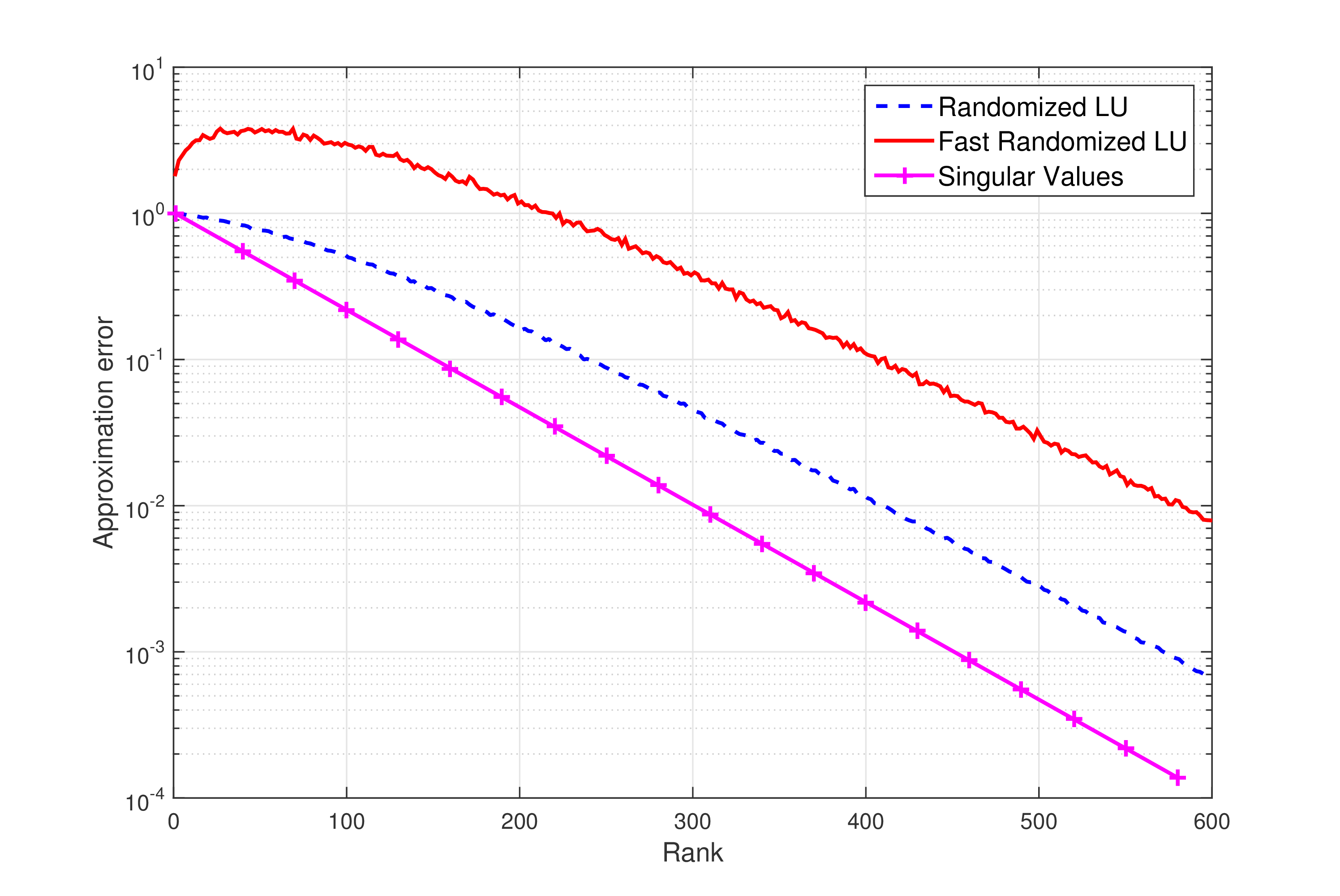
The experiment from section 5.1 was repeated, with a slowly decaying singular values. The decay of the singular values is the same as was used for the power iterations comparison $\sigma_{k}=\frac{100}{(9+k)^{2}}$ . These results appear in Fig. 5.13

The reason the error of the fast randomized LU is larger than the error of the randomized LU is due to the fact that the space from which the projections are chosen is much smaller than the space created by the Gaussian-based random projection. The space is smaller since the projection matrix contains only a random diagonal matrix and a random column selection matrix. This large error is also reflected in the error bounds of the algorithm (Theorem 4.12) and also in the need for a larger $l$ compared to $k$ (Lemma 4.13).

Conclusion

In this work, we presented a randomized algorithm for computing an LU rank $k$ decomposition. Given an integer $k$ , the algorithm finds an LU decomposition where both $L$ and $U$ are of rank $k$ with negligible failure probability. Error bounds for the approximation of the input matrix were derived, and were proved to be proportional to the ( $k+1$ )th singular value. The performance of the algorithm (error and computational time) was compared to the randomized SVD, randomized ID and to the application of Lanczos SVD. We also showed that the algorithm can be parallelized since it consists mostly of matrix multiplication and pivoted LU. The results on GPU show that it is possible to reduce the computational time significantly by even using only the standard MATLAB libraries.

Acknowledgment

This research was partially supported by the Israel Science Foundation (Grant No. 1041/10), by the Israeli Ministry of Science & Technology (Grants No. 3-9096, 3-10898), by US - Israel Binational Science Foundation (BSF 2012282) and by a Fellowship from Jyväskylä University. The authors would like to thank Yoel Shkolnisky for the helpful discussions.

References

[1] Dimitris Achlioptas and Frank Mcsherry. Fast computation of low-rank matrix approximations. Journal of the ACM (JACM), 54(2):9, 2007.
[2] N. Ailon and B. Chazelle. The fast Johnson–Lindenstrauss transform and approximate nearest neighbors. SIAM J. Computing, 39(1):302–322, 2009.
[3] Haim Avron, Petar Maymounkov, and Sivan Toledo. Blendenpik: Supercharging LAPACK’s least-squares solver. SIAM Journal on Scientific Computing, 32(3):1217–1236, 2010.
[4] A. Bermanis, A. Averbuch, and R.R. Coifman. Multiscale data sampling and function extension. Applied and Computational Harmonic Analysis, 34:15–29, 2013.
[5] Rajendra Bhatia. Matrix analysis, volume 169. Springer, 1997.
[6] Christos Boutsidis and Alex Gittens. Improved matrix algorithms via the subsampled randomized Hadamard transform. SIAM Journal on Matrix Analysis and Applications, 34(3):1301–1340, 2013.
[7] Tony F Chan. Rank revealing QR factorizations. Linear Algebra and Its Applications, 88:67–82, 1987.
[8] Zizhong Chen and Jack J Dongarra. Condition numbers of Gaussian random matrices. SIAM Journal on Matrix Analysis and Applications, 27(3):603–620, 2005.
[9] H. Cheng, Z. Gimbutas, P.G. Martinsson, and V. Rokhlin. On the compression of low rank matrices. SIAM Journal on Scientific Computing, 26(4):1389–1404, 2005.
[10] Kenneth L Clarkson and David P Woodruff. Numerical linear algebra in the streaming model. In Proceedings of the 41st annual ACM symposium on Theory of computing, pages 205–214. ACM, 2009.
[11] Kenneth L Clarkson and David P Woodruff. Low rank approximation and regression in input sparsity time. In Proceedings of the 45th annual ACM symposium on Symposium on theory of computing, pages 81–90. ACM, 2013.
[12] Ronald R. Coifman and Stéphane Lafon. Diffusion maps. Applied and Computational Harmonic Analysis, 21(1):5–30, 2006.
[13] G. David. Anomaly Detection and Classification via Diffusion Processes in Hyper-Networks. PhD thesis, School of Computer Science, Tel Aviv University, March 2009.
[14] Timothy A Davis and Iain S Duff. An unsymmetric-pattern multifrontal method for sparse LU factorization. SIAM Journal on Matrix Analysis and Applications, 18(1):140–158, 1997.
[15] James W Demmel, Stanley C Eisenstat, John R Gilbert, Xiaoye S Li, and Joseph WH Liu. A supernodal approach to sparse partial pivoting. SIAM Journal on Matrix Analysis and Applications, 20(3):720–755, 1999.
[16] David L Donoho. Compressed sensing. Information Theory, IEEE Transactions on, 52(4):1289–1306, 2006.
[17] Petros Drineas, Ravi Kannan, and Michael W Mahoney. Fast monte carlo algorithms for matrices II: Computing a low-rank approximation to a matrix. SIAM Journal on Computing, 36(1):158–183, 2006.
[18] Petros Drineas, Michael W Mahoney, and S Muthukrishnan. Relative-error CUR matrix decompositions. SIAM Journal on Matrix Analysis and Applications, 30(2):844–881, 2008.
[19] Michael Elad and Michal Aharon. Image denoising via sparse and redundant representations over learned dictionaries. Image Processing, IEEE Transactions on, 15(12):3736–3745, 2006.
[20] Alan Frieze, Ravi Kannan, and Santosh Vempala. Fast monte-carlo algorithms for finding low-rank approximations. Journal of the ACM (JACM), 51(6):1025–1041, 2004.
[21] Herman H Goldstine and John Von Neumann. Numerical inverting of matrices of high order II. Proceedings of the American Mathematical Society, 2(2):188–202, 1951.
[22] Gene H Golub and Charles F Van Loan. Matrix computations, volume 4. John Hopkins University Press, 2012.
[23] Ming Gu and Stanley C Eisenstat. Efficient algorithms for computing a strong rank-revealing QR factorization. SIAM Journal on Scientific Computing, 17(4):848–869, 1996.
[24] Nathan Halko, Per-Gunnar Martinsson, and Joel A Tropp. Finding structure with randomness: Probabilistic algorithms for constructing approximate matrix decompositions. SIAM review, 53(2):217–288, 2011.
[25] David Kirk. nVidia CUDA software and GPU parallel computing architecture. In ISMM, volume 7, pages 103–104, 2007.
[26] Yehuda Koren, Robert Bell, and Chris Volinsky. Matrix factorization techniques for recommender systems. Computer, 42(8):30–37, 2009.
[27] RM Larsen. Lanczos bidiagonalization with partial reorthogonalization. Technical Report DAIMI PB-357, Department of Computer Science, Aarhus University, 1998.
[28] AE Litvak and O Rivasplata. Smallest singular value of sparse random matrices. Stud. Math, 212:195–218, 2010.
[29] Alexander E Litvak, Alain Pajor, Mark Rudelson, and Nicole Tomczak-Jaegermann. Smallest singular value of random matrices and geometry of random polytopes. Advances in Mathematics, 195(2):491–523, 2005.
[30] Avner Magen and Anastasios Zouzias. Low rank matrix-valued chernoff bounds and approximate matrix multiplication. In Proceedings of the Twenty-Second Annual ACM-SIAM Symposium on Discrete Algorithms, pages 1422–1436. SIAM, 2011.
[31] Per-Gunnar Martinsson, Arthur Szlam, and Mark Tygert. Normalized power iterations for the computation of svd. Manuscript., Nov, 2010.
[32] P.G. Martinsson, V. Rokhlin, and M. Tygert. A randomized algorithm for the decomposition of matrices. Applied and Computational Harmonic Analysis, 30(1):47–68, 2011.
[33] Rahul Mazumder, Trevor Hastie, and Robert Tibshirani. Spectral regularization algorithms for learning large incomplete matrices. The Journal of Machine Learning Research, 99:2287–2322, 2010.
[34] L Miranian and M Gu. Strong rank revealing LU factorizations. Linear algebra and its applications, 367:1–16, 2003.
[35] C-T Pan. On the existence and computation of rank-revealing LU factorizations. Linear Algebra and its Applications, 316(1):199–222, 2000.
[36] Vladimir Rokhlin and Mark Tygert. A fast randomized algorithm for overdetermined linear least-squares regression. Proceedings of the National Academy of Sciences, 105(36):13212–13217, 2008.
[37] Mark Rudelson and Roman Vershynin. Smallest singular value of a random rectangular matrix. Communications on Pure and Applied Mathematics, 62(12):1707–1739, 2009.
[38] Olaf Schenk, Klaus Gärtner, and Wolfgang Fichtner. Efficient sparse LU factorization with left-right looking strategy on shared memory multiprocessors. BIT Numerical Mathematics, 40(1):158–176, 2000.
[39] Gil Shabat, Yaniv Shmueli, Amit Bermanis, and Amir Averbuch. Accelerating particle filter using randomized multiscale and fast multipole type methods. IEEE Transactions on Pattern Analysis and Machine Intelligence, 37(7):1396–1407, 2015.
[40] GW Stewart. The triangular matrices of gaussian elimination and related decompositions. Technical Report TR-3533, Department of Computer Science and Institute for Advanced Computer Studies, University of Maryland, College Park, MD, 1995.
[41] GW Stewart. The decompositional approach to matrix computation. Computing in Science & Engineering, 2(1):50–59, 2000.
[42] Lloyd N Trefethen and Robert S Schreiber. Average-case stability of gaussian elimination. SIAM Journal on Matrix Analysis and Applications, 11(3):335–360, 1990.
[43] Joel A Tropp. Improved analysis of the subsampled randomized hadamard transform. Advances in Adaptive Data Analysis, 3(01n02):115–126, 2011.
[44] Rafi Witten and Emmanuel Candes. Randomized algorithms for low-rank matrix factorizations: sharp performance bounds. Algorithmica, pages 1–18, 2013.
[45] Lior Wolf and Amnon Shashua. Learning over sets using kernel principal angles. The Journal of Machine Learning Research, 4:913–931, 2003.
[46] F. Woolfe, E. Liberty, V. Rokhlin, and M. Tygert. A fast randomized algorithm for the approximation of matricess. Applied and Computational Harmonic Analysis, 25(3):335–366, 2008.

Randomized LU Decomposition

Abstract

Keywords:

1 Introduction

2 Related Work

3 Preliminaries

3.1 Rank Revealing LU (RRLU)

Theorem 3.1 ([35]).

Definition 3.1 (RRLU Rank kk Approximation denoted RRLUk).

Lemma 3.2 (RRLU Approximation Error).

Proof.

Lemma 3.3 ([5]).

Lemma 3.4 ([32]).

3.2 Subgaussian Random Matrices

Definition 3.2.

Definition 3.3.

Theorem 3.5 ([29]).

Theorem 3.6 ([29]).

3.3 The SRFT matrix

Lemma 3.7 ([46]).

3.4 Interpolative decomposition (ID)

4 Randomized LU

Remark 4.1.

Remark 4.2.

Theorem 4.3.

4.1 Computational Complexity Analysis

4.2 Bounds for the Randomized LU (Proof of Theorem 4.3)

Lemma 4.4.

Proof.

Lemma 4.5 ([32]).

Lemma 4.6.

Proof.

Remark 4.7.

Remark 4.8.

Proof of Theorem 4.3.

Remark 4.9.

Theorem 4.10.

Proof.

4.3 Analysis of the bound in Theorem 4.10

Corollary 4.11 ([24]).

4.4 Rank Deficient Least Squares

4.5 Fast Randomized LU

4.5.1 Computational complexity

4.5.2 Correctness Algorithm 4.4

Theorem 4.12.

Lemma 4.13.

Lemma 4.14.

Proof.

Lemma 4.15 (Appears in [46] as Lemma 4.6).

Lemma 4.16.

Proof.

Proof.

5 Numerical Results

5.1 Error Rate and Computational Time Comparisons

5.2 Power Iterations

5.3 Image Matrix Factorization

5.4 Fast Randomized LU

Conclusion

Acknowledgment

References

Definition 3.1 (RRLU Rank $k$ Approximation denoted RRLU_k).