Using concatenated algebraic geometry codes in channel polarization

The performance of the polar code is determined based on the asymptotic error probability. In Arikan’s construction of a binary polar code [2] using the matrix $G_{2}$, the asymptotic error probability of the polar code using the successive cancellation decoding is

The error probability $P_{\operatorname{err}}$ above¹¹ 1 The parameter $\beta$ is an arbitrary real number, if $\beta<1/2$, then there exists a polar code that satisfies $P_{\text{err}}=o\left(2^{-N^{\beta}}\right)$ is independent of the rate $R$ of the polar code. Mori and Tanaka [19] extended the formula above to one that is rate dependent. Moreover, the threshold $1/2$ depends only on the matrix $G_{2}$ and not on the underlying channel $W$.

Now for any $\ell\times\ell$ matrix $G$ that polarizes the $q$-ary input S-DMC $W$, the asymptotic error probability of the polar code is given by

for some well-defined constant $E(G)\in[0,1)$ depending only on the matrix $G$ and not on the underlying channel $W$. The quantity $E(G)$ is called the exponent of the matrix $G$. It measures the performance of the polar code under successive cancellation decoding ([10, Section IV] for $q=2$ and [13, Theorem 9] for any $q>2$).

As mentioned in the previous subsection, the exponent of the matrix $G$ plays an important role in determining the performance of the polar codes. In [10],[14], the authors gave an algebraic description of the exponent in terms of the partial distances of the matrix $G$.

For $q$-ary codes, Mori and Tanaka [14] suggested using algebraic geometry codes in order to get larger exponents. The motivation behind this idea is the Reed-Solomon code which gives large exponents. In particular, algebraic geometry codes have in general large minimum distance and often they have a nested structure similar to the Reed-Solomon code which makes them suitable for channel polarization.

In this section we introduce the concatenation of codes which is illustrated in the following theorem.

The code $C_{1}$ in Theorem 11 is called the outer code, the code $C_{2}$ is called the inner code, and the code $C$ is called the concatenated code. In the following, we will use the descent code $(\mathbb{F}_{q})^{m}$ which is a $(m,m,1)$-linear code as an inner code and all field extensions $\mathbb{F}_{q}$ are of characteristic 2. Therefore, given a $(N,K,D)$-linear code over $\mathbb{F}_{2^{m}}$, Theorem 11 yields a binary $(mN,mK,D)$-linear code.

Let $G\in\text{Mat}({L},{L},{\mathbb{F}_{q}})$ be a generating matrix for a code over $\mathbb{F}_{q}$ and let $(D_{1},\dots,D_{L})$ be its profile. Recall that the exponent of $G$ is given by

Applying the inner code $(m,m,1)$ to the matrix $G$ will replace each symbol in $G$ with $m$ binary symbols and each row will be redundant $m$ times. Therefore, the new concatenated matrix, denoted by $G_{2}$, will be of size $mL\times mL$, and will have at least the following profile

Then, the exponent of the binary matrix $G_{2}$ satisfies the inequality

Mori and Tanaka [14] evaluated the performance of polar codes using kernels constructed from the generating matrices of the Reed-Solomon and Hermitian codes over a $q$-ary field. They have found that numerically Hermitian codes give larger exponents than Reed-Solomon codes. That suggests using different algebraic geometry codes as they have large minimum distance and often have the same nested structure as Reed-Solomon codes. We continue in this direction by using algebraic geometry codes to study the behavior of the exponent. In Section 3 we show for a subclass of algebraic geometry codes, that $E(G_{L})\to 1$ as the number of affine rational points $L\to\infty$.

In Section 4 we will apply the concatenation of codes to construct binary codes from $q$-ary codes. As the algebraic geometry codes are defined over different field extensions of $\mathbb{F}_{2}$. This helps us to study the performance of different algebraic geometry codes defined over a common field which is the binary field $\mathbb{F}_{2}$. We will study numerically whether to use larger field extensions or curves with many rational points to get a larger exponent. In other words, it is the study of how to approach $\infty$ in the most efficient way using either concatenation or geometry. In the first case (concatenation) we would need codes defined over large fields and in the second case (geometry) we would need curves with many rational points defined over small fields.

In Section 5 we compare numerically how the Reed-Solomon, Hermitian, and Suzuki codes behave in the settings above for a given binary block size. It turns out that each code will give the maximum exponent for some range of the binary block size, and that more geometry is preferable as the block size increases. We also compare their performance as error-correcting codes.

Let $X/\mathbb{F}_{q}$ be a curve (smooth, irreducible, and projective) of genus $g$ over $\mathbb{F}_{q}$ with global function field $F:=\mathbb{F}_{q}(X)$. Let $X(\mathbb{F}_{q})$ be the set of all $\mathbb{F}_{q}$-rational points on $X$ with cardinality $N(F)$. Let $1\leq n<N(F)$ and choose $n$ distinct rational places $P_{1},\dots,P_{n}\in X(\mathbb{F}_{q})$. Set $D:=P_{1}+\dots+P_{n}$ and let $G^{\prime}:=\sum_{i=1}^{s}n_{i}Q_{i}-\sum_{j=1}^{t}m_{j}Q^{\prime}_{j}\in\operatorname{Div}(X)$ ($n_{i},m_{j}\in\mathbb{N}$) be a divisor of $X$ such that $\operatorname{Supp}(D)\cap\operatorname{Supp}(G^{\prime})=\phi$. Define the Riemann-Roch space $\mathcal{L}(G^{\prime})$ to be the $\mathbb{F}_{q}$-vector space of all rational functions $f\in F$ which are having only poles at $Q_{i}$ of order less than or equal to $n_{i}$ and zeros at $Q^{\prime}_{i}$ of order greater than or equal to $m_{j}$, i.e.,

Then, the algebraic geometry code is defined as

The code $C_{\mathcal{L}}(D,G^{\prime})$ is a $(n,k,d)$-linear code over $\mathbb{F}_{q}$, where $k:=\ell(G^{\prime})-\ell(G^{\prime}-D)$ and $d\geq d^{*}:=n-\deg(G^{\prime})$. Moreover, assume $n>\deg(G^{\prime})$ and let $\{f_{1},\dots,f_{k}\}$ be a basis for $\mathcal{L}(G^{\prime})$ over $\mathbb{F}_{q}$. Then, $C_{\mathcal{L}}(D,G^{\prime})$ has the following generator matrix

In this section we use Stirling’s formula to show that $E(G_{L})\to 1$ as $L\to\infty$, where $G_{L}$ is the generating matrix of an algebraic geometry code of block length $L$. First we state the Oesterlé bound (see [7, Theorem 8, page 130]) which gives a lower bound to the genus $g$ of a curve $X/\mathbb{F}_{q}$ with $L$ affine rational points. Let $\ell$ be the unique integer such that $\sqrt{q}^{\ell}<L\leq\sqrt{q}^{\ell+1}$, i.e.,

We find

Next, we find $\theta\in\left[\pi/(\ell+1),\pi/\ell\right)$ such that

Then, the Oesterlé bound is the lower bound

Note that for some small $L$, this bound can be achieved by maximal curves over $\mathbb{F}_{q^{2}}$ or for large $L$ by towers of function fields. We will study the case where $g:=\left((L-1)\sqrt{q}\cos\theta+q-L\right)/\left(q+1-2\sqrt{q}\cos\theta\right)$.

Now we prove the result of this section. Here we will study only the subclass of algebraic geometry codes over $\mathbb{F}_{q}$ with a matrix $G_{L}\in\text{Mat}({L},{L},{\mathbb{F}_{q}})$ that has profile²² 2 The least possible profile for a nested structure AG code using the point at infinity

Therefore,

Let $n$ be a fixed binary block size. Then, $L=L(m)=n/m$ and $\theta=\theta(m)$ can be found using (7). This means that $E_{2}(G)$ can be written in term of $m$. Numerically using Mathematica, enumerating over all positive integers $m$ shows that $E_{2}(G)$ has a local maximum, e.g., see Figure 1 and Table 1 for binary block size $n=3\cdot 2^{20}$.

In Section 5, numerically as $n$ gets larger, this local maximum corresponds first to the Reed-Solomon code for a small range of $n$, then it corresponds to the Hermitian code and as $n$ gets larger, the local maximum corresponds to the Suzuki code (see Figure 5).

Let $\theta$ be fixed, i.e., the underlying algebraic curve is fixed. Then, $L=L(m)$ can be found in terms of $m$ as follows. Find $\ell:=\ell(\theta)=\left\lfloor\pi/\theta\right\rfloor$, using (7) we have

Then, using (6), we get

Therefore, $E_{2}(G)$ is a function of $m$. In this case it turns out that $E_{2}(G)$ is an increasing function (see Figure 2). This means that more concatenation gives larger exponents.

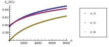
Let $m$ be fixed. Using (7), $\theta=\theta(L)$ and so $E_{2}(G)$ can be regarded as a function of $L$. Numerically $E_{2}(G)$ is an increasing function in $L$ with limit that tends to $1$ as $L\to\infty$ (see Figure 3). This means again that more geometry gives larger exponents.

As the rate of polarization is determined based on the exponent of the kernel, we compare numerically the three codes above as suitable kernels for channel polarization. Let $n$ be the binary block size, we draw a graph between the values of $n$ and the corresponding values of $E_{2}(G)$ for the three codes (see Figure 4).

From the graph we notice that as $n$ gets larger, the maximum $E_{2}(G)$ is attained first by the Reed-Solomon codes for values of $n<1800$, after that as $n$ gets larger, by the Hermitian codes up to $n=399,212$ and after that by the Suzuki codes. This can be generalized to any $\theta=k\pi/\ell$, i.e., more geometry yields larger exponents as $n\to\infty$. We summarize this result in Figure 5.

In this section we compare the performance of the three codes above as error-correcting codes with fixed binary rate. We draw a graph between the binary block size $n$ and $(k+d)/n$, where $n$, $k$, and $d$ are the parameters of the binary concatenated code with fixed binary rate.

For that, let $C$ be an algebraic geometry code with parameters $(L,K,D)$ over $\mathbb{F}_{2^{m}}$ constructed from the algebraic curve of genus $g$ with $L$ affine rational points. Then, we have

Assume $(K+D)/L=(L-g+1)/L$ [20, Corollary 4.1.14, p. 196]. Then, the concatenated binary code has parameters $(mL,mK,d^{\prime})(d^{\prime}\geq D)$. Therefore,

Therefore, we can draw the graph between $n$ and $(k+d)/n$ as in Figure 6.

Figure 6 shows that as $n\to\infty$, $(k+d)/n\to R=1/2$ and for the first few values of $n$, the Reed-Solomon code is the closest code to the line $y=1/2$, then comes the Hermitian code to be the closest and as $n$ gets larger, the Suzuki code is the code that is closest to the line $y=1/2$, so we have once again that more geometry is preferable as the block size increases.

References

- [1] E. Arikan, Channel polarization: A method for constructing capacity-achieving codes, Information Theory, 2008. ISIT 2008. IEEE International Symposium on, july 2008, pp. 1173–1177.
- [2] E. Arikan and E. Telatar, On the rate of channel polarization, Information Theory, 2009. ISIT 2009. IEEE International Symposium on, 28 2009-july 3 2009, pp. 1493–1495.
- [3] William Feller, An introduction to probability theory and its applications. Vol. I, Third edition, John Wiley & Sons Inc., New York, 1968. MR 0228020 (37 #3604)
- [4] G.D. Forney, Concatenated codes, M.I.T. research monograph no. 37, Mit Press, 1966.
- [5] Naveen Goela, Emmanuel Abbe, and Michael Gastpar, Polar codes for broadcast channels, CoRR abs/1301.6150 (2013).
- [6] J. P. Hansen and H Stichtenoth, Group codes on certain algebraic curves with many rational points, Appl. Algebra Engrg. Comm. Comput. 1 (1990), no. 1, 67–77. MR 1325513 (96e:94023)
- [7] N. Hurt, Many rational points, coding theory and algebaic geometery, Kluwer Academic Publishers, Dordrecht, The Netherlands, 2003.
- [8] N. Hussami, R. Urbanke, and S.B. Korada, Performance of polar codes for channel and source coding, Information Theory, 2009. ISIT 2009. IEEE International Symposium on, 28 2009-july 3 2009, pp. 1488–1492.
- [9] Wolfram Research Inc, Mathematica edition: Version 8.0 publisher: Wolfram research, inc, Third edition, John Wiley & Sons Inc., Champaign, Illinois, 2010.
- [10] S.B. Korada, E. Sasŏglu , and R. Urbanke, Polar codes: Characterization of exponent, bounds, and constructions, Information Theory, IEEE Transactions on 56 (2010), no. 12, 6253–6264.
- [11] Xudong Ma, Symbol-index-feedback polar coding schemes for low-complexity devices, CoRR abs/1201.1462 (2012).
- [12] Hessam Mahdavifar and Alexander Vardy, Achieving the secrecy capacity of wiretap channels using polar codes, CoRR abs/1007.3568 (2010).
- [13] R. Mori and T. Tanaka, Channel polarization on q-ary discrete memoryless channels by arbitrary kernels, Information Theory Proceedings (ISIT), 2010 IEEE International Symposium on, june 2010, pp. 894–898.
- [14] , Non-binary polar codes using reed-solomon codes and algebraic geometry codes, Information Theory Workshop (ITW), 2010 IEEE, 30 2010-sept. 3 2010, pp. 1–5.
- [15] Ryuhei Mori and Toshiyuki Tanaka, Source and channel polarization over finite fields and reed-solomon matrix, CoRR abs/1211.5264 (2012).
- [16] C. Xing S. Ling, Coding theory, a first course, Cambridge, Cambridge, UK, 2004.
- [17] Eren Sasoglu, Emre Telatar, and Erdal Arikan, Polarization for arbitrary discrete memoryless channels, CoRR abs/0908.0302 (2009).
- [18] H. Stichtenoth, Algebraic function field and code, Springer, Berlin, 2009.
- [19] T. Tanaka and R. Mori, Refined rate of channel polarization, Information Theory Proceedings (ISIT), 2010 IEEE International Symposium on, june 2010, pp. 889–893.
- [20] Michael Tsfasman, Serge Vlăduţ, and Dmitry Nogin, Algebraic geometric codes: basic notions, Mathematical Surveys and Monographs, vol. 139, American Mathematical Society, Providence, RI, 2007. MR 2339649 (2009a:94055)