Eight light flavors on large lattice volumesThanks: Present address

Many-flavor lattice calculations are carried out at stronger bare couplings than QCD, which requires appropriate improvement of the lattice action. Our gauge action includes an adjoint plaquette term with coefficient $\beta_{A}=-\beta_{F}/4$ (so that perturbatively $\beta_{F}\simeq 12/g^{2}$), and we use staggered fermions improved with one step of nHYP smearing. The nHYP smearing parameters are $\alpha=(0.5,0.5,0.4)$, small enough to avoid numerical instabilities. Taking advantage of previous studies of this action [12, 13], we focus our attention on $\beta_{F}=5.0$, a relatively strong coupling that is still weak enough to avoid a lattice phase.

We have implemented this action in QHMC (a.k.a. FUEL, ‘‘Framework for Unified Evolution of Lattices’’), a USQCD software package currently under development. QHMC is being designed to allow flexible experimentation with integration algorithms. To generate large-volume configurations on Intrepid, we use an HMC algorithm with two to four Hasenbusch masses, depending on the volume and fermion mass. Subsequent measurements (e.g., of the Wilson flow, spectrum and eigenvalues) are carried out on clusters using code based in part on the MILC Collaboration’s public lattice gauge theory software.⁴⁴ 4 http://www.physics.utah.edu/$∼$detar/milc/

Our volumes vary from $16^{3}\!\times\!32$ to $64^{3}\!\times\!128$, with overlapping ranges of fermion masses $m$ that we use to monitor finite-volume effects. Table 1 lists our ensembles, reporting the number of molecular dynamics time units (MDTU) accumulated as of October 2013. The initial target for each ensemble is $\sim$3000 MDTU, to provide ample statistics after thermalization. In addition, two $24^{3}\!\times\!48$ ensembles (with $m=0.02$ and 0.015) and one $32^{3}\!\times\!64$ ensemble (with $m=0.01$) are being extended to $\sim$10,000 MDTU for investigations of glueballs and the scalar spectrum.

Regarding thermalization, we have found Wilson flow observables measured after long flow times $t$ to be sensitive probes of thermalization (more so than $\left\langle\overline{\psi}\psi\right\rangle$, for example). The Wilson flow integrates out to distances $\sim\sqrt{8t}$, providing relatively inexpensive long-range quantities. Fig. 1 shows representative time-series plots for the energy $E$ and topological charge $Q$,

both constructed from the clover-leaf definition of $F_{\mu\nu}$. Such time-series plots of $t^{2}E$ indicate that most ensembles thermalize within 300 MDTU. The lighter-mass $48^{3}\!\times\!96$ ensembles take longer to thermalize, 400 MDTU for $m=0.008$ and 0.006, and 450 MDTU for $m=0.004$. We anticipate that the $64^{3}\!\times\!128$ ensembles will require $\sim$500 MDTU for thermalization.

The left panel of Fig. 1 shows that the gauge fields evolve significantly from the initial configuration. Subsequent auto-correlation times should therefore be shorter than the time for the runs to thermalize. The right panel of Fig. 1 reinforces this expectation, demonstrating healthy fluctuations in the topological charge from Eq. 1, with topological susceptibility $\chi_{t}$ roughly quadratic in $m$.

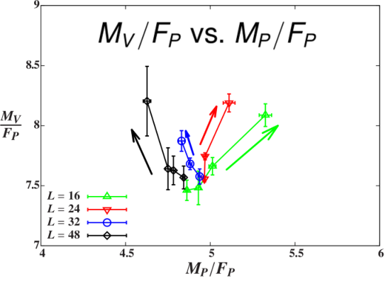
Let us first consider which of our ensembles may be subject to significant finite-volume effects. The left panel of Fig. 2 plots $M_{V}/F_{P}$ vs. $M_{P}/F_{P}$, where $M_{V}$ ($M_{P}$) is the vector (pseudoscalar) meson mass and $F_{P}$ is the pseudoscalar decay constant. These ratios are designed to emphasize finite-volume effects, which we expect to increase $M$ while decreasing $F_{P}$, pushing the points up and to the right. Such behavior is clearly visible for the lightest $16^{3}\!\times\!32$ and $24^{4}\!\times\!48$ points, while the larger volumes move up and to the left for smaller $m$. In systems exhibiting spontaneous chiral symmetry breaking (S$\chi$SB), we would expect these ratios to move the left as $m$ decreases, since $M_{P}\to 0$ while the other quantities remain non-zero. We may be seeing initial signs of such behavior in Fig. 2, though this is not yet clear, even for $m=0.004$ on a $48^{3}\!\times\!96$ volume.

Another way of searching for S$\chi$SB in these data is to plot $M_{V}/M_{P}$ vs. $M_{P}$, as in the right panel of Fig. 2. If $M_{V}$ remains non-zero in the chiral limit, this ratio diverges as $M_{P}\to 0$. Only the lightest $48^{3}\!\times\!96$ point shows a significant increase, ending up about 16% larger than the heaviest $24^{3}\!\times\!48$ point. This $48^{3}\!\times\!96$ ensemble with $m=0.004$ is currently our shortest run, has our longest thermalization time, and may suffer from finite-volume effects. The $64^{3}\!\times\!128$ runs in Table 1 seem to be required in order to access the chiral regime.

We can also see this by considering the right panel of Fig. 3, which presents chiral extrapolations of $F_{P}$. Simple linear extrapolations give $F\equiv\lim_{m\to 0}F_{P}=0.021(2)$, so that $L\gtrsim 50$ is required to satisfy $FL\gtrsim 1$. All linear and power-law fits shown in Fig. 3 use the following six points:

By omitting either or both the lightest ($m=0.004$) and heaviest ($m=0.02$) data points, we observe significant dependence on the fit range, which dominates the current uncertainty on $F$.

The power-law fits have smaller $\chi^{2}$ than the linear extrapolations, typically by an order of magnitude or more, for the same number of degrees of freedom. Writing the power as $M\propto m^{1/(1+\gamma_{m})}$, we find $\gamma_{m}=0.76(2)$ for $M_{P}$, while $\gamma_{m}=0.95(5)$ for $M_{V}$ and $\gamma_{m}=0.92(3)$ for $F_{P}$, again with uncertainties dominated by the fit range in $m$. (As mentioned in the previous section, $\chi_{t}\propto m^{4/(1+\gamma_{m})}$ with $\gamma_{m}=0.76(10)$.) Finite-size scaling, using all 14 thermalized ensembles in Table 1, prefers slightly smaller values: $\gamma_{m}=0.732(2)$ for $M_{P}$, $\gamma_{m}=0.86(2)$ for $M_{V}$ and $\gamma_{m}=0.779(3)$ for $F_{P}$.

In the chiral limit, the chiral condensate $\Sigma=\lim_{m\to 0}\left\langle\overline{\psi}\psi\right\rangle$ is the order parameter of S$\chi$SB. We can probe $\Sigma$ in three ways, all of which are shown in the right panel of Fig. 4, normalized per continuum flavor. Direct measurements of $\left\langle\overline{\psi}\psi\right\rangle$ are dominated by a term $\propto m/a^{2}$, requiring a long extrapolation to the chiral limit. Using the spectrum results discussed above, we apply the Gell-Mann–Oakes–Renner (GMOR) relation $\left\langle\overline{\psi}\psi\right\rangle=M_{P}^{2}F_{P}^{2}/(2m)$ to obtain another estimate that turns out to be less sensitive to $m$.

Finally, the Banks–Casher relation $\Sigma=\lim_{\lambda\to 0}\ \lim_{m\to 0}\ \lim_{V\to\infty}\pi\rho(\lambda)$ allows us to extract the chiral condensate from the eigenvalue density of the massless Dirac operator. The left panel of Fig. 4 shows representative data for $\rho(\lambda)$, on different volumes with fixed dynamical fermion mass $m_{s}=0.01$. There are clear finite-volume effects in the $24^{3}\!\times\!48$ results (which we already saw in Fig. 2), but $\rho(\lambda)$ for the larger volumes is roughly constant over a range of $\lambda$. We estimate this constant by calculating the slope of its integral, the eigenmode number $\nu(\lambda)\propto\int_{0}^{\lambda}\rho(\omega)d\omega$. We have not attempted to remove any near-zero modes associated with the fluctuating topological charge shown in Fig. 1; for now we simply omit the first few bins of $\rho(\lambda)$ from our analysis.

The chiral extrapolations in the right panel of Fig. 4 all produce very small $\Sigma$, the largest being $\Sigma_{dir}=9(2)\times 10^{-4}$ from direct measurements. In fact, when extrapolated linearly in $m_{s}$, the GMOR and eigenvalue results both lead to negative $\Sigma$. Although Fig. 4 shows $m_{s}\to 0$ extrapolations, linear fits in terms of $M_{P}^{2}$ are much more stable for the GMOR and eigenvalue results (but not for the direct measurements or $M_{V}$ and $F_{P}$ discussed above). From such $M_{P}^{2}\to 0$ extrapolations, we find $\Sigma_{eig}=0.55(5)\times 10^{-4}$, while $\Sigma_{GMOR}=-1.5(7)\times 10^{-4}$ is still slightly negative. As in the previous section, these uncertainties are dominated by dependence on the fit range. The points listed in Eq. 2 correspond to $0.016<M_{P}^{2}<0.11$, while omitting the lightest and heaviest points gives $0.025<M_{P}^{2}<0.073$. In short, we cannot reliably resolve a non-zero chiral condensate, even using $48^{3}\!\times\!96$ ensembles with fermion masses as light as $m=0.004$ ($M_{P}=0.13$).

The results discussed above only scratch the surface of the physics potential in the eight-flavor ensembles being generated by USBSM. Already we see that this system has a very small or vanishing chiral condensate, and the light hadron spectrum correspondingly shows no clear signs of spontaneous chiral symmetry breaking. We identify where finite-volume effects are under control, and observe well-behaved thermalization and auto-correlations in the configuration generation.

In addition, we are carrying out valence domain wall measurements on ensembles with $m\geq 0.008$, to study the electroweak $S$ parameter following the methods of Ref. [10]. We have also developed unitary staggered measurements of the vector and axial-vector correlation functions that determine $S$, to see if the computational cost of valence domain wall measurements is truly justified. The scalar spectrum is another high priority that we are actively investigating, with the extended $24^{3}\!\times\!48$ and $32^{3}\!\times\!64$ ensembles our first targets for glueball and disconnected diagram calculations.

Intrepid will retire at the end of 2013, by which time we hope to complete all of our $48^{3}\!\times\!96$ ensembles, and obtain thermalized configurations for at least one $64^{3}\!\times\!128$ run. Given our current results for the spectrum and $\Sigma$, especially the preliminary value $F=0.021(2)$, such a $64^{3}\!\times\!128$ ensemble will be extremely valuable in our attempt to access the chiral regime.

I thank the participants in the USBSM community for collaboration and review of this contribution. In particular, George Fleming, Anna Hasenfratz, Meifeng Lin, James Osborn and Ethan Neil made important contributions to the work summarized above, which also benefited from conversations with Kieran Holland and Julius Kuti. Part of this work was performed at the Aspen Center for Physics (NSF Grant No. 1066293), which I thank for support and hospitality. Partial support came from DOE Grant Nos. DE-SC0010005, DE-FC02-12ER41877 and DE-FG02-85ER40231. In addition to gauge generation on Intrepid, numerical analyses were carried out on clusters at Argonne, Livermore and Fermilab, the last managed by USQCD with support from the DOE.

References

- [1] T. Appelquist, G. T. Fleming and E. T. Neil, Phys. Rev. Lett. 100 (2008) 171607 [arXiv:0712.0609]; Phys. Rev. D79 (2009) 076010 [arXiv:0901.3766].
- [2] A. Deuzeman, M. P. Lombardo and E. Pallante, Phys. Lett. B670 (2008) 41–48 [arXiv:0804.2905].
- [3] Z. Fodor, K. Holland, J. Kuti, D. Nogradi and C. Schroeder, Phys. Lett. B681 (2009) 353–361 [arXiv:0907.4562].
- [4] A. Hasenfratz, Phys. Rev. D82 (2010) 014506 [arXiv:1004.1004].
- [5] X.-Y. Jin and R. D. Mawhinney, PoS Lattice 2010 (2010) 055 [arXiv:1011.1511].
- [6] A. Cheng, A. Hasenfratz, G. Petropoulos and D. Schaich, JHEP 1307 (2013) 061 [arXiv:1301.1355].
- [7] LatKMI Collaboration: Y. Aoki, T. Aoyama, M. Kurachi, T. Maskawa, K.-i. Nagai, H. Ohki, A. Shibata, K. Yamawaki and T. Yamazaki, Phys. Rev. D87 (2013) 094511 [arXiv:1302.6859].
- [8] LatKMI Collaboration: Y. Aoki, T. Aoyama, M. Kurachi, T. Maskawa, K. Miura, K.-i. Nagai, H. Ohki, E. Rinaldi, A. Shibata, K. Yamawaki and T. Yamazaki, arXiv:1309.0711.
- [9] T. Appelquist, R. Brower, S. Catterall, G. Fleming, J. Giedt, A. Hasenfratz, J. Kuti, E. Neil and D. Schaich, USQCD White Paper (2013) [arXiv:1309.1206].
- [10] LSD Collaboration: T. Appelquist, R. Babich, R. C. Brower, M. Cheng, M. A. Clark, S. D. Cohen, G. T. Fleming, J. Kiskis, M. Lin, E. T. Neil, J. C. Osborn, C. Rebbi, D. Schaich and P. Vranas, Phys. Rev. Lett. 106 (2011) 231601 [arXiv:1009.5967].
- [11] LSD Collaboration: T. Appelquist, R. Babich, R. C. Brower, M. I. Buchoff, M. Cheng, M. A. Clark, S. D. Cohen, G. T. Fleming, J. Kiskis, M. Lin, E. T. Neil, J. C. Osborn, C. Rebbi, D. Schaich, S. Syritsyn, G. Voronov, P. Vranas and J. Wasem, Phys. Rev. D85 (2012) 074505 [arXiv:1201.3977].
- [12] A. Cheng, A. Hasenfratz and D. Schaich, Phys. Rev. D85 (2012) 094509 [arXiv:1111.2317].
- [13] A. Hasenfratz, A. Cheng, G. Petropoulos and D. Schaich, arXiv:1303.7129.