Tension moderation and fluctuation spectrum in simulated lipid membranes under an applied electric potential

We model the membrane as a smooth two-dimensional surface with height above the xy-plane $h(x,y)$. We will model the effect of the electric field to be equivalent to adding a term proportional to the area in the free energy. In order to describe the effects of this additional tension we will follow the approach of [11] and take the following Hamiltonian:

$$\mathcal{H}=\mathcal{H}_{c}+\mathcal{H}_{s}+\mathcal{H}_{\rm add}$$

(1)

where $\mathcal{H}_{c}$ is the Helfrich bending energy:

$$\mathcal{H}_{c}=\int\mathrm{d}A\ \frac{\kappa}{2}\left(2H\right)^{2}$$

(2)

here the integral is over the whole area $A$ of the membrane, $H$ is the local mean curvature (half the sum of the principal curvatures) and $\kappa$ is the bending rigidity of the membrane, i.e., its resistance to bending. $\mathcal{H}_{s}$ is the contribution from the elastic stretching of the membrane. It reads:

$$\mathcal{H}_{s}=\frac{K_{a}}{2A_{0}}\left(A-A_{0}\right)^{2}$$

(3)

where $K_{a}$ is the area expansion modulus and $A_{0}$ is a the preferred area of the membrane. Finally $\mathcal{H}_{\rm add}$ is the contribution from an additional intrinsically applied tension $\sigma_{\rm add}$:

$$\mathcal{H}_{\rm add}=\sigma_{\rm add}A$$

(4)

In our simulations $\sigma_{\rm add}$ is taken to be the contribution from the applied electric potential. The membrane surface can be expanded in a series of complex exponentials:

$$h(x,y)=\sum_{q_{x}}\sum_{q_{y}}\tilde{h}(q_{x},q_{y})e^{i(xq_{x}+yq_{y})}$$

(5)

where $\tilde{h}$ are the corresponding expansion coefficients and $q_{x}$ and $q_{y}$ are wavenumbers in the $x$ and $y$ directions of the membrane, they can take the values:

$$q_{x}=n_{x}\frac{2\pi}{L_{x}}\quad{\rm and}\quad q_{y}=n_{y}\frac{2\pi}{L_{y}}$$

(6)

where $L_{x}$ and $L_{y}$ are the box size in the $x$ and $y$ direction and $n_{x}$ and $n_{y}$ are integers. In this approach the microscopic nature of the membrane is ignored and it is necessary to introduce a cut off for both $n_{x}$ and $n_{y}$ such that $\left|q_{x}\right|\leq q_{\rm max}$ and $\left|q_{y}\right|\leq q_{\rm max}$ where the wavelength corresponding to $q_{\rm max}$ is the wavelength at which the continuous description of the membrane breaks down. These restrictions on the values of $q_{x}$ and $q_{y}$ are implied throughout the paper. The fluctuation spectrum is defined as the average value of the square of the absolute value of $\tilde{h}$ at equilibrium. Using standard statistical mechanics, the fluctuation spectrum can be shown to be [12]:

$$\left<|\tilde{h}(q)|^{2}\right>=\frac{k_{B}T}{L_{x}L_{y}}\frac{1}{\tilde{\sigma}q^{2}+\kappa q^{4}}$$

(7)

where this expression depends only on the norm of the wavevector $q=\sqrt{q_{x}^{2}+q_{y}^{2}}$. The brackets mean an ensemble average which is equivalent to a time average at equilibrium. $\tilde{\sigma}$ is an is a moderated tension that depends on $\sigma_{\rm add}$, $K_{a}$, $\kappa$ and the tension $\sigma_{0}$ of the membrane when $\sigma_{\rm add}=0$. According to [11] $\tilde{\sigma}$ can be calculated self-consistently using the equation:

$$\tilde{\sigma}-\sigma_{\rm add}=K_{a}\frac{\left<A\right>-A_{0}}{A_{0}}$$

(8)

If we want to use the projected area, $L_{x}L_{y}$, instead of $A_{0}$ we rewrite this equation as:

$$\tilde{\sigma}-\sigma_{\rm add}=K_{a}u\left(\alpha(\tilde{\sigma})+1-\frac{1}{u}\right)$$

(9)

where $u=L_{x}L_{y}/A_{0}$ (see the supplementary material for values of $u$ in our simulations) and $\alpha$ is the fractional excess area defined as:

$$\alpha=\frac{\left<A\right>-L_{x}L_{y}}{L_{x}L_{y}}=\sum_{q_{x}}\sum_{q_{y}}\frac{1}{2}q^{2}\left<|\tilde{h}(q)|^{2}\right>$$

(10)

The final tension is then the sum of the additional applied tension plus an elastic contribution and must be determined self-consistently. This elastic contribution will moderate the applied tension. Note that if we had assumed an equation of the form of $\mathcal{H}_{\rm add}$ for $\mathcal{H}_{s}$ instead, say $\mathcal{H}_{s}=\sigma_{0}A$, the tension after adding $\mathcal{H}_{\rm add}$ would simply be $\tilde{\sigma}=\sigma_{\rm add}+\sigma_{0}$ i.e. there would be no elastic response of the membrane to the external additional stress. In this paper we verify the elastic moderation of the tension through molecular dynamics simulations. In particular we will apply an electric potential difference, $V$, across our membranes. This electric potential will give rise to stress in the membrane in the form of an additional tension $\sigma_{\rm add}$. In order to try to quantify this effect we use Eq. 9 making the following assumption for $\sigma_{\rm add}$. The membrane we simulate is symmetrical, so the first non-zero term in an expansion in $V$ of $\sigma_{\rm add}$ is quadratic. This means that, to lowest order:

$$\sigma_{\rm add}=\mu V^{2}$$

(11)

where $\mu$ is a phenomenological constant that depends on the membrane composition, but also on the ionic concentration and the water properties. In the following we will use Eq. (9) together with (11) in order to explain the observed behavior of our membranes.

The Martini coarse grained force field [13] has been used to perform simulations of a membrane bilayer. In order to observe large wavelength fluctuations the simulated membrane was made rectangular by duplicating a equilibrated patch of membrane in the $x$ direction. This patch was then equilibrated and duplicated again until we reached the desired size. The final system consisted of 602964 particles as 4224 POPC molecules, 181884 water beads, 1200 sodium ions and 1200 chloride ions. For the water, the polarizable water model of Martini has been used [14], note that this include a background permittivity of $2.5\epsilon_{0}$. We use an ionic concentration of $\sim 90\ {\rm mM}$ which was chosen such that the membrane would be electrically screened from its periodic images (the Debye length [15] is on the order of $1\ {\rm nm}$). All simulations were run at a temperature of 325 K in order to accelerate fluctuation dynamics. We performed the simulation in the ${\rm NP_{z}AT}$ ensemble where the pressure normal to the membrane is fixed to one bar and the projected area of the membrane is fixed in the lateral direction. This allows us to directly observe the change in the fluctuations and the tension due to the applied electric potential.

We note here that we chose the Martini force field because it gives a good trade off between performance and accuracy. Furthermore the polarizable water version of it gives a reasonable value for the dielectric permittivity of water. It is known, however, that the electrical potential in the membrane (i.e. the so called dipole electrical potential) is negative with respect to the bulk fluid in Martini simulations. Experimental evidence suggest that it is actually positive for real lipid membranes [16, 17]. This problem has already been noted in the original paper for the polarizable Martini water [14], but is not an issue here because the electrostatic stresses are proportional to the square of the electric field and do not depend on its sign.

The fluctuation spectrum is calculated and convergence is checked as explained below. Our original membrane patch was $132.18\times 10.93\times 19.04$ ${\rm nm^{3}}$. From this we constructed three other patches with the following scaling factor on the x axis: $0.996$, $1.02$ and $1.05$, resulting in boxes of length $131.71$, $134.82$ and $138.79\ {\rm nm}$ respectively. In the following we will refer to these different cases by their scaling factor. The stretched membrane was obtained by scaling the coordinates of all residues in the system. No stable system could be obtained by scaling the the coordinates of all residues for the shrunk membrane so we used the following method: we relaxed the constraint on the fixed size of the simulation box in the x direction while fixing the size in the z direction after creating a small vacuum above and below the membrane. The system then automatically shrank in order to conserve its volume, we obtained a box size of $131.71\times 10.93\times 19.11$ ${\rm nm^{3}}$ which is close to a 0.996 factor ($0.99644$). For each of these patches two initial sets of velocities were used to run two sets of simulations. They were first equilibrated with Berendsen coupling for the temperature and the pressure [18] and then subsequently run with the Nose-Hoover [19, 20] thermostat and the Parrinello-Rahman [21, 22] barostat. All electrostatics was handled using the Particle Mesh Ewald (PME) method [23, 24] using the parameters for the polarizable water model [14]. Subsequently we applied transmembrane potentials of $200\ {\rm mV}$ and $500\ {\rm mV}$. We did so by applying a uniform external electric field $E_{\rm ext}$ along the z axis in the simulation box such that $V=E_{\rm ext}L_{z}$ where $V$ is the applied electric potential and $L_{z}$ the average box height [25], giving an applied electric field no greater than $E_{\rm ext}\approx 27.5\ {\rm mV/nm}$. All simulations were performed using GROMACS 4.5.5 [26, 27, 28].

We express each leaflet of the bilayer by a continuous surface expressed in terms of an expansion in complex exponentials:

	$\displaystyle z_{\rm up}(x,y,z)$	$\displaystyle=\sum_{q_{x}}\sum_{q_{y}}\tilde{z}_{\rm up}(q_{x},q_{y})e^{i(xq_{x}+yq_{y})}$		(12)
	$\displaystyle z_{\rm dw}(x,y,z)$	$\displaystyle=\sum_{q_{x}}\sum_{q_{y}}\tilde{z}_{\rm dw}(q_{x},q_{y})e^{i(xq_{x}+yq_{y})}$		(13)

where $z_{\rm up}$ ($z_{\rm dw}$) is the smooth surface associated with the upper (lower) layers, the $\tilde{z}_{\rm up}$ ($\tilde{z}_{\rm dw}$) are the corresponding coefficients in the expansion.This means for the corresponding expansion coefficients of $\tilde{h}$:

$$\tilde{h}(q_{x},q_{y})=\frac{1}{2}\left(\tilde{z}_{\rm up}(q_{x},q_{y})+\tilde{z}_{\rm dw}(q_{x},q_{y})\right)$$

(14)

The fluctuation spectrum can then be compared with Eq. (7). In our simulation the tension can be measured directly by calculating the difference between the normal and the lateral pressure:

$$\gamma=L_{z}\left(P_{zz}-\frac{1}{2}(P_{xx}+P_{yy})\right)$$

(15)

where $L_{z}$ is the box length in the $z$ direction and $P_{zz}$ is the normal and $P_{xx}$ and $P_{yy}$ are the lateral components of the averaged pressure tensor. The bending rigidity can then be inferred from the calculated fluctuation spectrum. In this paper we will assume that $\gamma=\tilde{\sigma}$, i.e., that the mechanical lateral stress acting on the membrane is the same as the tension in the fluctuation spectrum. However we point out that this issue is still controversial to this day [29, 30, 31, 32, 33, 34].

In contrast to previously used methods like the direct Fourier sum [35] and the binning technique [36, 37], we obtained the fluctuation spectrum by using a least square fit with cosines and sines to the PO4 (the phosphate group) particle positions for each leaflet (see the supplementary material [38]). This is certainly a similar technique to the one used in [39] but no details can be found in this publication. We note that if all the data points are evenly spaced in the simulation box, then the least square method is completely equivalent to the discrete Fourier transform applied on those points. In the range of wavenumbers we used for the calculations of the bending rigidity, the difference between the different methods is expected to be negligible. In particular we will only use the points for which $q_{y}=0$ and $q<0.5\ {\rm nm^{-1}}$ (see the supplementary material for a justification[38]). We will postpone a discussion on this matter for a future publication. Note that choosing the PO4 particles as the definition of the layer surface is somewhat arbitrary, however we have verified that choosing another reference particle does not change the results obtained here. This is because we are looking at the average of the position between the upper and lower layer, Eq.(14), and the specifics of the contributions cancel.

For all our simulations, we checked the convergence of our fluctuation spectrum by looking at the distribution of the $|\tilde{h}(q)|^{2}$ after an equilibration period. Indeed, at equilibrium, a number of variables of the system will fluctuate around their mean values and have a Gaussian distribution. The $h$ variable is one such variable of the system and therefore the distribution of the $|\tilde{h}(q)|^{2}$ should be exponential. In order to quantitatively evaluate the convergence we compared the mean values of the $|\tilde{h}(q)|^{2}$ to their standard deviations. For an exponential distribution these two quantities are equal. The main limiting factor for the convergence of the fluctuation spectrum is the simulation time, which must be large enough in order for the largest wavelength fluctuation to sufficiently sample their phase space. The convergence criteria we chosed is that the difference between the mean and standard deviation of the fluctuations be no more than $15\%$ of the value of the mean. This criterium for convergence have been applied to all of our simulations. We believe this is the first time such a convergence test is applied to membrane fluctuations in molecular dynamics simulations and we expect it to be useful for future studies.

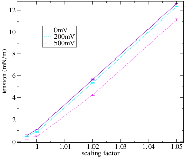
In Table 1 we show the thickness, bending rigidity and mechanical tension we measured in our different simulations. As the membrane is stretched, the tension increases. In Figure 1 we plot the tension as a function of the projected area (in our case as a function of the stretching factor as we only stretch in one direction) for all our simulations. When one increases the projected area of a fluctuating membrane, one will first pull out the excess area from the fluctuations and only at a later point will one actually start to stretch the membrane. In the region where the membrane is stretched one can recover the area expansion modulus $K_{a}$ [40, 41]. We have only used the points for $1.00$, $1.02$ and $1.05$ in order to calculate $K_{a}$. We obtained $K_{a}\sim 224.8\pm 7{\rm mN/m}$ which is quite comparable to the experimental value $213\pm 5\ {\rm mN/m}$ [42].

We show the fluctuation spectra for our simulations without an applied electric potential in Fig. 2. Note that the overall amplitude of the fluctuation decreases as the membrane is stretched, indicating that the excess area of the membrane decreases, see Eq. (10). According to Eq. (7) the fluctuation spectrum will essentially show two regimes depending on the value of $q$: for $q\ll\sqrt{\tilde{\sigma}/\kappa}$ the fluctuation spectrum becomes independent of the bending rigidity and is proportional to $1/(\tilde{\sigma}q^{2})$, for $q\gg\sqrt{\tilde{\sigma}/\kappa}$ it reaches a regime independent of the tension and proportional to $1/(\kappa q^{4})$ and for $q\sim\sqrt{\tilde{\sigma}/\kappa}$ the fluctuation should have a behavior between a $q^{-2}$ and a $q^{-4}$ line. We can see on the figure that in the $q^{-2}$ regime of the fluctuation spectra are decreasing as the scaling factor is increased. This is coherent with the increase of the tension we observe in Table 1. We can then obtain the bending rigidity by fitting the fluctuation spectra. Using the mechanical tension $\gamma$ for $\sigma_{0}$, box side lengths and temperature as measured in our simulations, the bending rigidity is our only fitting parameter in Eq.(7). The results are presented in Table 1. Within the error bars the bending rigidity for the $0.996$ and $1.00$ case are similar but it is clearly decreased for the $1.02$ and $1.05$ case. The decrease of the bending rigidity can be related to a decrease in the thickness of the membrane (see [43] for a discussion). The value we obtained for the $1.00$ case is $\kappa\approx 10.5\times 10^{-20}\ \mathrm{J}$ and can be compared to an experimental value $15.8\times 10^{-20}\ \mathrm{J}$ [42] at $25\ {\rm{}^{\circ}C}$ without salt. Note that both the increase in temperature and the addition of salt is expected to decrease the bending rigidity [44, 45] so the agreement is expected to be better for the bending rigidity for a high temperature membrane ($325\ {\rm K}$) with a large salt concentration ($\sim 100{\rm mM}$). We are unaware of another measurement for the bending rigidity of POPC membrane using molecular dynamics simulations. We can however compare the value we obtained to the value obtained using the same (Martini) force field in [35, 46]. They found $\kappa\approx 15\times 10^{-20}\ \mathrm{J}$ for a DPPC and DMPC membrane. Only one double bond in the carbon chain is not expected to make a big difference for the bending rigidity [43].

Next we apply an electric potential difference across our membranes. We use two values for the electric potential, 200mV and 500mV, and we measure the tension, thickness and by fitting the fluctuation spectrum we get the bending rigidity (Table 1). Generally an applied electric field tend to squeeze the membrane and hence decrease the tension, as expected from theory [3, 10, 47]. We plot the fluctuation spectrum we obtained for the 1.00 case for 0, 200 and $500\ {\rm mV}$ in Figure 3. The amplitude of the large wavelength fluctuation should increase because the tension decreases. This is clearly the case with the $500\ {\rm mV}$ applied electric potential, but it is not so clear with the $200\ {\rm mV}$ applied electric potential as the first mode is found to have a lower amplitude than the $0\ {\rm mV}$ in some cases. Also, we observed no net increase or decrease of the bending rigidity with the applied electric potential and we were unable to observe a change in thickness. We conclude that, within error bars, the bending rigidity is not affected by the applied electric potential for the salt concentration we use in the simulations. Theory [3, 10] predict a contribution much lower than $k_{B}T$ in accordance with our observation. Finally a note on the observed thickness. We do not observe any thickness change when we apply the electric potential, see Table 1. A quick calculation, assuming that the membrane conserves its volume, shows that the thickness change should be proportional to $1-(1+\alpha_{1})/(1+\alpha_{2})$ if the membrane area changes from $\alpha_{1}$ to $\alpha_{2}$. In our case this induces a change in thickness which is less than $0.2\%$ and is bellow the error bars in Table 1. Electro-compressive stresses translate into a membrane tension decrease but it is unclear from our data if there is a thickness change. This will depend on the elastic properties of the membrane as a 3 dimensional medium.

Our main result is that the tension contribution from the applied electric potential is moderated depending on the initial tension of the membrane. We calculate the difference between the measured tension with an applied electric potential, $\gamma$, and the initial tension with zero electric potential, $\sigma_{0}$, for all our different scaling factors. Using Eq. (9) together with Eq. (7) we then find the value for $\sigma_{\rm add}$ that minimizes the squared error with the values obtained in our simulations. In Figure 4 we show the values extracted from our simulations as well as the fitted values of $\sigma_{\rm add}$. We obtained $\sigma_{\rm add}=-0.31\ {\rm mN/m}$ for $200\ {\rm mV}$ and $\sigma_{\rm add}=-1.55\ {\rm mN/m}$ for $500\ {\rm mV}$. As can be seen on the figure the contribution to the tension vanishes when $\sigma_{0}$ is below a critical tension $\sigma_{c}$ and takes its full effect only for a sufficiently stretched membrane. According to [11] $\sigma_{c}$ can be estimated as $\sigma_{c}\approx K_{a}k_{\rm B}T/(8\pi\kappa)$. Taking the average of the bending rigidity values in Table 1, $\kappa\approx 9.75\times 10^{-20}\ \mathrm{J}$, we get $\sigma_{c}\approx 0.43\ {\rm mN/m}$. In the inset of Figure 4 we fitted the values of $\sigma_{\rm add}$ to Eq. (11). We obtained $\mu\approx-6.2\ {\rm mN/m/V^{2}}$.

Furthermore, using the equation for the tension with a large salt concentration given in [3], one can estimate $\mu\approx-\varepsilon/2d$ where $\varepsilon$ is the dielectric constant in the membrane and $2d$ the thickness of the membrane. One could have guessed this equation by assuming that the membrane behaves like a capacitor of dielectric constant $\varepsilon$ and of thickness $2d$. Using $\varepsilon\approx 2.5\varepsilon_{0}$, where $\varepsilon_{0}$ is the vacuum permittivity, and $2d\approx 4.4\ {\rm nm}$ we get $\mu\approx-5.0\ {\rm mN/m/V^{2}}$, in fair agreement with our obtained values.

Next we calculate $\sigma_{\rm add}$ directly by identifying it with minus the Maxwell stresses created by the applied electric potential. In order to evaluate this contribution we can calculate the electric field given by the average charge distribution over the z axis. Assuming that the electric field is uniform on the $x$ and $y$ direction, the Maxwell stress can be calculated as:

$$T_{\rm M,zz}=-T_{\rm M,xx}=-T_{\rm M,yy}=\varepsilon_{0}\frac{1}{2}\left(E_{\rm norm}\right)^{2}$$

(16)

where $E_{\rm norm}$ is the integral of the average of the charge density in the $x$ and $y$ direction $\left<\rho\right>_{x,y}$:

$$E_{\rm norm}(z)=\frac{1}{\varepsilon_{0}}\int_{0}^{z}\mathrm{d}\tilde{z}\ \left<\rho\right>_{x,y}(\tilde{z})$$

(17)

We show the electric field obtained that way in figure Fig.5 for our 1.00 simullations. The electrostatic contribution to the tension can then be evaluated as:

	$\displaystyle\sigma_{\rm el}$	$\displaystyle=-\int\mathrm{d}z\ \left(T_{\rm M,zz}-\frac{1}{2}\left(T_{\rm M,xx}+T_{\rm M,yy}\right)\right)$		(18)
		$\displaystyle=-\varepsilon_{0}\int\mathrm{d}z\ \left(E_{\rm norm}\right)^{2}$		(19)

where the integral is over the $z$ direction and $T_{\rm M,zz}$, $T_{\rm M,xx}$ and $T_{\rm M,yy}$ are respectively the normal and lateral Maxwell stresses. The additional contribution due to the applied potential can then be evaluated as:

$$\sigma_{\rm add}(V)=\sigma_{\rm el}(V)-\sigma_{\rm el}(0)$$

(20)

where $\sigma_{\rm el}(V)$ is the electrostatic tension calculated from Eq. (18) with an applied electric potential $V$. In Table 2 we calculated $\sigma_{\rm el}$ and $\sigma_{\rm add}$. We can see that for a given applied electric potential the absolute value of the different contributions of the applied electric potential to the stresses for the different scaling are the same within $10^{-2}\ {\rm mN/m}$. Furthermore we obtained $\sigma_{\rm add}\approx-0.27\pm 0.01\ {\rm mN/m}$ in the $200\ {\rm mV}$ case and $\sigma_{\rm add}\approx-1.72\pm 0.01\ {\rm mN/m}$ in the $500\ {\rm mV}$ case which compare well to the values we obtained from the fits of (9), see Figure 4. Also the electrostatic contribution found for the tension is on the order of (minus) the electrostatic stress found in an electroporation simulation ($1\approx 2\ mN/m$ for a potential range of $0.5\approx 1\ V$) [48]. Note however that further comparison are difficult because the membrane is porated is this simulation. The overall agreement between our calculated values suggests that the applied electrostatic stress does not change with the initial state of the membrane and that the moderation of the tension is a consequence of the elastic response of the membrane, due to all the non electrostatic interactions.

References

- [1] A. G. Lee, Biochim. Biophys. Acta 1666, 62 (2004).
- [2] R. Phillips, T. Ursell, P. Wiggins, and P. Sens, Nature 459, 379 (2009).
- [3] T. Ambjörnsson, M. A. Lomholt, and P. L. Hansen, Phys. Rev. E 75, 051916 (2007).
- [4] N. C. Gauthier, T. A. Masters, and M. P. Sheetz, Trends Cell Bio. 22, 527 (2012).
- [5] B. Loubet, U. Seifert, and M. A. Lomholt, Phys. Rev. E 85, 031913 (2012).
- [6] E. A. Evans and V. A. Parsegian, Proc. Natl. Acad. Sci. 83, 7132 (1986).
- [7] E. Reister-Gottfried, K. Sengupta, B. Lorz, E. Sackmann, U. Seifert, and A. S. Smith, Phys. Rev. Lett. 101, 208103 (2008).
- [8] M. D. E. A. Faris, D. Lacoste, J. Pecreaux, J.-F. Joanny, J. Prost, and P. Bassereau, Phys. Rev. Lett. 102, 038102 (2009).
- [9] H. Bouvrais, F. Cornelius, J. H. Ipsen, and O. G. Mouritsen, PNAS 109, 1844218446 (2012).
- [10] D. Lacoste, G. I. Menon, M. Z. Bazant, and J.-F. Joanny, Eur. Phys. J. E 28, 243 (2009).
- [11] M. A. Lomholt, B. Loubet, and J. H. Ipsen, Phys. Rev. E 83, 011913 (2011).
- [12] W. Helfrich, Z. Naturforsch. 28c, 693 (1973).
- [13] S. Marrink, H. Risselada, S. Yefimov, D. Tieleman, and A. de Vries, J. Phys. Chem. B 111, 78127824 (2007).
- [14] S. Yesylevskyy, L. Schafer, D. Sengupta, and S. Marrink, PLoS Comput Biol 6(6), 1000810 (2010).
- [15] P. Debye and E. Hückel, Phyzik Z. 24, 185 (1923).
- [16] H. Brockman, Chem. Phys. Lipids 73, 57 (1994).
- [17] Y. Yang, K. M. Mayer, N. S. Wickremasinghe, and J. H. Hafner, Biophys. J 95, 5193 (2008).
- [18] H. J. C. Berendsen, J. P. M. Postma, A. DiNola, and J. R. Haak, J. Chem. Phys. 81, 36843690 (1984).
- [19] S. A. Nose, Mol. Phys. 52, 255268 (1984).
- [20] W. G. Hoover, Phys. Rev. A 31, 16951697 (1985).
- [21] M. Parrinello and A. Rahman, J. Appl. Phys. 52, 71827190 (1981).
- [22] S. Nose and M. L. Klein, Mol. Phys. 50, 10551076 (1983).
- [23] T. Darden, D. York, and L. Pedersend, J. Chem. Phys. 98, 1008910092 (1993).
- [24] U. Essmann, L. Perera, M. L. Berkowitz, T. Darden, H. Lee, and L. G. Pedersen, J. Chem. Phys. 103, 85778592 (1995).
- [25] J. Gumbart, F. Khalili-Araghi, M. Sotomayor, and B. Roux, BBA-Biomembranes 1818, 294 (2012).
- [26] H. Bekker, H. J. C. Berendsen, E. J. Dijkstra, S. Achterop, R. van Drunen, D. van der Spoel, A. Sijbers, H. Keegstra, B. Reitsma, and M. K. R. Renardus, Physics Computing 92: Gromacs: A parallel computer for molecular dynamics simulations (R A De Groot J Nadrchal, 1993).
- [27] H. J. C. Berendsen, D. van der Spoel, and R. van Drunen, Comp. Phys. Comm. 91, 43 (1995).
- [28] B. Hess, C. Kutzner, D. van der Spoel, and E. Lindahl, J. Chem. Theory Comp. 4(3), 435 (2008).
- [29] O. Farago and P. Pincus, Eur. Phys. J. 11, 399 (2003).
- [30] O. Farago and P. Pincus, J. Chem. Phys. 120, 2934 (2004).
- [31] A. Imparato, J. Chem. Phys. 124, 154714 (2006).
- [32] J.-B. Fournier and C. Barbetta, Phys. Rev. Lett. 100, 078103 (2008).
- [33] O. Farago, Phys. Rev. E 84, 051914 (2011).
- [34] F. Schmid, EPL 95, 28008 (2011).
- [35] E. G. Brandt, A. R. Braun, J. N. Sachs, J. F. Nagle, and O. Edholm, Biophys. J. 100, 21042111 (2011).
- [36] E. Lindahl and O. Edholm, Biophys. J. 79, 426 (2000).
- [37] M. C. Watson, E. S. Penev, P. M. Welch, and F. L. H. Brown, J. Chem. Phys. 135, 244701 (2011).
- [38] See supplementary material at [URL will be inserted by AIP] for details on the technique used.
- [39] J. Stecki, J. Chem. Phys. 137, 116102 (2012).
- [40] E. Evans and W. Rawicz, Physical Review Letters 64, 2094 (1990).
- [41] Q. Waheed and O. Edholm, Biophys. J. 97, 2754 (2009).
- [42] J. Henriksen, A. C. Rowat, E. Brief, Y. W. Hsueh, J. L. Thewalt, M. J. Zuckermann, and J. H. Ipsen, Biophys. J. 90, 1639 (2006).
- [43] W. Rawicz, K. C. Olbrich, T. McIntosh, D. Needham, and E. Evans, Biophysical Journal 79, 328 (2000).
- [44] J. Pan, S. Tristram-Nagle, N. Kucěrka, and J. F. Nagle, Biophys. J. 94, 117 (2008).
- [45] M. M. A. E. Claessens, B. F. van Oort, F. A. M. Leermakers, F. A. Hoekstra, and M. A. C. Stuart, Biophys. J. 87, 3882 (2004).
- [46] M. C. Watson, E. G. Brandt, P. M. Welch, and F. L. H. Brown, Phys. Rev. Lett. 109, 028102 (2012).
- [47] J. C. Weaver and Y. Chizmadzhev, Bioelectroch. Bioener. 41, 135 (1996).
- [48] M. Tarek, Biophys. J. 88, 4045 (2005).
- [49] P. Moe and P. Blount, Biochem. 44, 12239 (2005).
- [50] M. P. Sheetz and J. Dai., Trends Cell Biol. 6, 85 (1996).
- [51] J. Dai, H. P. Ting-Beall, and M. P. Sheetz, J. Gen. Physiol. 110, 1 (1997).
- [52] D. P. Tieleman, BMC Biochem. 5, 10 (2004).
- [53] M. Tokman, J. Lee, Z. Levine, M.-C. Ho, and M. Colvin, PLoS ONE 8, e61111 (2013).