Dual-fermion approach to interacting disordered fermion systems
Abstract
We generalize the recently introduced dual fermion (DF) formalism for disordered fermion systems by including the effect of interactions. For an interacting disordered system the contributions to the full vertex function have to be separated into crossing-asymmetric and crossing-symmetric scattering processes, and addressed differently when constructing the DF diagrams. By applying our approach to the Anderson-Falicov-Kimball model and systematically restoring the nonlocal correlations in the DF lattice calculation, we show a significant improvement over the Dynamical Mean-Field Theory and the Coherent Potential Approximation for both one-particle and two-particle quantities.
pacs
71.27.+a, 02.70.-c, 71.10.Fd, 71.23.AnI Introduction
The transport and thermodynamic properties of many real materials are strongly influenced by disorder and strong electron correlations [1, 2]. The interplay of these two effects can lead to many interesting novel phenomena. In particular, both disorder and electron-electron interactions are known to be the driving mechanisms for metal-insulator transitions, although of different nature. Electron correlations induce the Mott-Hubbard metal-insulator transition with the opening of a gap in the single particle excitation spectrum [3]. On the other hand, coherent back-scattering of electrons off disorder-induced non-periodic potentials can lead to their localization, known as Anderson localization [4]. Despite intensive studies, the proper modeling of disordered interacting systems remains a great challenge.
Mean field methods like the coherent potential approximation (CPA) [5, 6, 7, 8] and the dynamical mean field theory (DMFT) [9, 10, 11, 12, 13] have revolutionized the study of disordered and correlated systems. These are single-site mean field approximations with an averaged local momentum-independent effective medium. As single-site methods, both the CPA and DMFT fail to take into account non-local correlations, which are found to be important in many cases. For example, in correlated clean systems one frequently observes ordered states with non-local order parameters which cannot be accounted for within the DMFT. Likewise, for non-interacting disordered systems it is well known that the CPA, while being rather successful describing electronic structures, completely fails to capture Anderson localization [1].
There have been a number of attempts to develop systematic nonlocal extensions to the CPA and DMFT. These include such cluster extensions as the Molecular Coherent Potential Approximation (MCPA) [14, 15, 16], Dynamical Cluster Approximation (DCA) [17, 18, 19], Cluster Coherent Potential Approximation (CCPA) [20, 21, 22, 23, 24], and the Traveling Cluster Approximation (TCA) [25, 26]. These methods generally extend the CPA and DMFT by replacing the single-site impurity problem by that of a finite-size cluster coupled to a mean field bath.
A distinctly different approach called the Dual Fermion (DF) method has been developed to incorporate non-local correlations introduced by both disorder and interactions. Originally constructed for interacting clean systems[27], it has been recently extended to study disordered non-interacting electronic systems [28] and disordered dipole system [29]. Note that earlier a very similar idea using parquet method has also been proposed by Janis [30], though DF method is more elegant, systematic, and most importantly, it designs an exact mapping from real fermion lattice onto dual fermion lattice. In this work, we extend the dual fermion approach further so both disorder and interaction effects can be be treated on equal footing. By separating the scattering vertex contributions into crossing-asymmetric and crossing-symmetric components, we manage to derive the proper DF mapping and construct the DF Feynman diagrams, which are now more complicated due to the different scattering processes arising from disorder and Coulomb interaction, respectively. We apply the method to the Anderson-Falicov-Kimball model. Our numerical results for 1D systems show a remarkable correction to the DMFT-CPA results and are consistent with DCA calculations of large clusters. Finally, the phase diagram for 2D systems is determined by using both one- and two-particle quantities.
The paper is organized as follows: in Section II we describe the details of the DF formalism for treating both disorder and electron-electron interactions. Results for one- and two-particle properties obtained from applying our DF formalism to the Anderson-Falicov-Kimball Model and how they compare with DMFT-CPA data are presented in Sec. III. Section IV summarizes and concludes the paper.
II Formalism
II.1 Dual fermion mapping
The paradigm for studying disordered correlated systems is the Anderson-Hubbard model
| (1) |
where is the dispersion of the band electrons, is the chemical potential, is the Coulomb interaction and the on-site disorder potential is distributed according to some given probability density . The latter can have in principle any form, but for the present purpose we specify it as
| (2) |
where is the step function
| (3) |
and is the disorder strength.
Following the derivation of the dual fermion mapping for the non-interacting disordered case [28], after introducing the auxiliary dual fermion degrees of freedom and then integrating out the real fermion degrees of freedom (see appendix for details), one arrives at an effective action (to simplify the notation we represent the fermionic Matsubara frequency as and bosonic Matsubara frequency as in the following)
| (4) |
in which the bare dual Green function is defined as the difference of lattice Green function and impurity Green function
| (5) |
and the dual potential (by keeping only the lowest two-body interaction)
| (6) | |||||
is split into crossing-asymmetric, with interaction strength , and crossing-symmetric terms, with interaction strength . They are parametrized by the real fermion full vertex
| (7) |
and will be detailed in section II.3. Note that in the above expression for the dual potential, a prefactor instead of is used for the crossing-asymmetric part because it does not have the full crossing-symmetries and thus can not be anti-symmetrized; while the crossing-symmetric part can be anti-symmetrized and thus carries a prefactor . When writing down the above concise expression for the dual fermion action, we have to impose the constraint that Hartree-like diagrams in the self-energy calculation constructed from should be eliminated at the one-particle level, while at the two-particle level the vertical component of the particle-hole (p-h) two-particle Green function should be canceled by the vacuum term. This constraint stems from taking the replica limit. [28, 19, 31] Both and are for the particle-particle (p-p) channel, and they are related to their counterparts for the particle-hole (p-h) channel by the crossing symmetry [32]
| (8) |
and
| (9) |
II.2 Algorithm
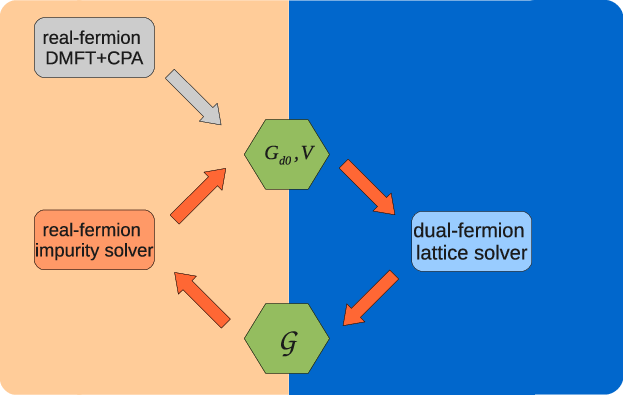
Like the conventional dual fermion algorithm for interacting systems, the dual fermion algorithm for an interacting disordered system can be represented schematically by Fig. 1. We start on the left side from a DMFT+CPA solution of the real fermion system, and then use the information collected by solving the impurity problem (mainly the one-particle Green function , self-energy , and two-particle Green function ) to parametrize the dual fermion system in the right half, i.e., construct the bare dual fermion Green function and the dual potential . While the local correlations are included in the DMFT+CPA solution, the nonlocal corrections are incorporated through the dual fermion part, which is calculated using a standard perturbation expansion in the term. After the dual fermion system is solved, we map it back to the real fermion system with the nonlocal corrections now included in the lattice self-energy and Green function . We then solve the impurity problem again starting with an updated impurity-excluded Green function . These steps are repeated until self-consistency is achieved with
| (10) |
i.e. with the local contribution to the dual fermion Green function being zero [27]. This condition would fix the arbitrary function introduced during the dual-fermion mapping in Appendix A and eliminate the first-order contribution to the self-energy on the dual-fermion lattice.
II.3 Dual potential
In the algorithm described above, the non-trivial part is the measurement of the two-particle Green functions. This is due to the requirement that the crossing-asymmetric and crossing-symmetric contributions must be separated and treated differently. We here propose a two-step procedure to measure the two-particle Green functions:
- •
quantum averaging (integrate out the Coulomb term)
- •
disorder averaging (integrate out the disorder term)
By this procedure, the crossing-asymmetric and crossing-symmetric components can be separated as detailed in the following.

In Fig. 2 (a) we show for the case of the p-h channel that the full two-particle Green function can be measured as (spin indices are suppressed to simplify the expressions, and hereafter, represents the one-particle Green function for a given decoupling field (for quantum averaging) and disorder configuration (for disorder averaging), while and are the fully dressed one-particle and two-particle Green functions respectively)
| (11) | |||||
in which the angle brackets represent the quantum averaging while the curly brackets represent the disorder averaging. The full vertex is defined according to the following equation
| (12) |
Similarly, as shown in Fig. 2 (b), we have
| (13) | |||||
for the p-p channel.
Note that the two-particle Green function measured in this manner still contains both the crossing-asymmetric and crossing-symmetric contributions. However, by analyzing the diagrams contributing to each component, we realize that the crossing-asymmetric component can be measured individually as (see Fig. 3 for the Feynman diagram)
| (14) |
The full vertex for the crossing-asymmetric component can then again be calculated using the definition equation
| (15) |
Let us now turn to the calculation of the crossing-symmetric component .

Diagrams for the full vertex are illustrated in Fig. 4, where the scattering from disorder is represented by a dashed line and black crosses, and the interaction by a wavy line. One obtains pure disorder diagrams (where only disorder scatterings appear in the connection of two fermion lines, only two frequencies are needed and thus can be expressed as ), pure interacting diagrams (only interaction scatterings in the connections) and the mixed diagrams:
| (16) |

To be able to do the calculation in the dual fermion formalism, one has to separate out the pure disorder contributions . Then the full vertex can be divided into two parts as shown in Fig. 5
| (17) |
with
| (18) |
and finally
| (19) | |||||
Note that while is fully crossing-symmetric and thus can be treated like a conventional vertex function in a clean interacting system, does not have full crossing symmetry. Specifically, each crossing symmetry involving the particle-hole vertical channel vertex is broken because that single channel contribution is absent from the construction.

III Results
To test our generalization of the dual fermion approach, we apply it to the simplest interacting disordered fermion system, the Anderson-Falicov-Kimball model
| (20) |
where is the dispersion for the itinerant c-electrons (only the nearest neighbor hopping is included), the on-site disorder potential follows the “box” probability distribution of Eq. (2) and U is the on-site Coulomb interaction between itinerant c-electrons and immobile f-electrons. In the limit of no Coulomb interaction, this model reduces to the Anderson disorder model and the dual-fermion calculation is presented in our previous contribution [28]. In the other limit of no disorder, it reduces to the Falicov-Kimball model for which both Quantum Monte Carlo and DCA results are available in the literature [33, 17, 18], and the dual fermion method is also applied on this model recently [34, 35].
In Sections III.1 and III.2 we will first look into corrections from the DF to the DMFT+CPA results on the one-dimensional (1D) lattice using the self-consistent second-order method to solve the DF lattice problem (DF-2nd) as an example (see Appendix C.3.2 for details). In Section III.3 we will carry out a detailed survey of the U-D phase-diagram for the two-dimensional (2D) lattice at a fixed temperature (with ) using DF-2nd and the fluctuation-exchange (FLEX) approximation to solve the DF lattice problem (DF-FLEX), see Appendix C.3.3 for additional details on the DF-FLEX approach. The filling is fixed at half-filling for both c- and f-electrons.
III.1 Local Green function


Figure 6 shows the Matsubara frequency dependence of the local Green function calculated from both DMFT+CPA and DF approaches for the 1D lattice at for zero and finite disorder strength at different temperatures . For clean system at U=0.8 and D=0 (Fig.6 (a)), both methods show an insulator-like behavior, which can be inferred from the imaginary part of the local Green function converging to zero as function of temperature for the lowest Matsubara frequency. However, while the DMFT+CPA results are temperature independent due to the neglect of the non-local correlations, there is a significant temperature dependence in the results from the DF approach. Moreover, they appear to be consistent with the DCA calculation for a cluster of size at included in Fig. 6 as filled black up-triangles.
Similarly, for finite disorder with (Fig. 6 (b)), the DF results recover the important temperature dependence from the non-local correlations, which are again absent in the DMFT+CPA calculation. Due to the disorder, the system becomes less insulating as compared to the clean case (contrast the lowest Matsubara frequency results in Fig. 6 and ). This is well-captured by the DF calculation which is also consistent with the DCA results, while the DMFT+CPA approach strongly over-estimates this effect.
III.2 Correction from the dual fermion calculation


In order to quantify how strong the corrections due to the non-local correlations from the DF approach are, we introduce the following quantity
| (21) |
which represents the relative difference of the imaginary part of the local Green function at the lowest Matsubara frequency. Results for the 1D lattice are shown in Fig. 7.
For both temperatures, T=0.02 (Fig. 7) and T=0.01 (Fig. 7), the corrections are weak in both small and large limits, reaching their maximum around , being the bandwidth. This verifies our belief that DMFT+CPA for the one-particle Green’s function works best for and , while for the kinetic and interaction parts of the Hamiltonian are strongly competing and non-local correlations become more important. Thus we will naturally expect an enhanced correction from the DF calculation in this region. The corrections are around 30 percent for T=0.02, and they increase to around 60 percent when the temperature is decreased to T=0.01. One interesting observation is that the peak in the plot shifts to larger U values and gradually smooths out when the disorder is increased.
III.3 U-D phase diagram for the two-dimensional lattice
Let us now turn to the phase diagram of the Anderson-Falicov-Kimball model.

An easy way to analyze the metal-insulator transition due to crossing-symmetric scattering processes from the Coulomb interaction is by looking at the difference between the imaginary part of the local Green function at the two lowest Matsubara frequencies:
| (22) |
When decreasing the temperature, the imaginary part of local Green function converges to zero for the insulating phase, while it diverges for the metallic phase. This different behavior can be captured with the above quantity, which is negative for the insulating phase, and positive for the metallic phase. Note that this distinction between metal and insulator phases is accurate only at zero temperature. For finite temperature, the insulator determined in this way could be just a bad metal in reality. So in the following, we will call it bad metal phase. The transition is actually a crossover indicated by the changing of the sign of . Fig. 8 shows the U-D phase diagram thus determined.
Both disorder and interaction tend to decrease the mobility of itinerant particles. However, in Fig. 8 only interaction drive the system to an insulating phase, while it remains metallic even for large disorder strength. This is due to the arithmetic averaging nature of the one-particle Green function within the DF approach, which does not distinguish between extended and localized electrons. The positive slope of the metal-bad-metal crossover line indicates that the disorder scattering helps particle mobility. Including more ladder-type diagrams, for example within a DF-FLEX calculation (Fig. 8), tends to move the crossover line to a smaller value of the interaction, and this shifting is less pronounced for larger disorder strengths.

To analyze the driving force of the metal-bad-metal crossover detected by the difference between the imaginary part of the two lower Matsubara frequencies local Green functions, we show in Fig. 9 the phase-diagram determined by the leading eigen-values (LEV) for the charge-density-wave (CDW) channel. The LEV is calculated by solving the eigen problem , where is the irreducible vertex and is the bare lattice susceptibility. Note that the closer the LEV is to unity, the more susceptible the system becomes to the CDW ordering. We can readily observe that the large-LEV region resembles the bad metal region in Fig. 8. This indicates that the metal-bad-metal crossover is driven by CDW correlations.

The phase-diagram determined from either or the LEV does not provide any signature of the Anderson localization. To cure such a deficiency, we turn to the dc conductivity (see Appendix C for the details of its calculation). In marked difference with the DMFT+CPA approach, the full vertex correction to the conductivity can be taken into account using the parquet equation. [28, 32] Results for this quantity are collected in Fig. 10, where we present the phase-diagram as determined by the conductivity.
In our calculation, the conductivity remains finite for all values of and on the 2D lattice. Therefore we use a small but finite conductivity value to delineate metallic and bad metal regions. This value is determined by matching the critical U for zero disorder strength to the one determined by , since both approaches should produce consistent result for the clean system. With this convention, we observe in Fig. 10 that the Anderson localization line connects continuously to the CDW metal-bad-metal crossover line. This is qualitatively similar to the ground-state phase-diagram obtained from the typical medium theory for the Bethe lattice [36, 37]. The difference is that the slope of the crossover line for small U is negative which indicates that the Coulomb interaction helps in localizing the particles.
IV Conclusion
We have generalized the recently proposed DF approach to treat both disorder and Coulomb interactions. This generalization is possible due to the clear separation between the crossing-asymmetric component, due to the disorder scattering, of the two-particle level vertex, and the crossing-symmetric component, due to the Coulomb interaction processes and the combined scattering processes from both disorder and Coulomb interactions. Thus the two competing factors can be treated on equal footing in this method.
We would like to emphasize that the separation and different treatments of crossing-asymmetric and crossing-symmetric scattering processes are generic for two-particle field-theory calculation of interacting disordered systems. Its application is not limited to the DF method proposed here, and instead might also find its use in other multi-scale diagrammatic methods, such as multi-scale many-boby approach [38] and dynamical vertex approximation [39].
To demonstrate the algorithm, we apply the method to the Anderson-Falicov-Kimball at half filling and compare our results to those obtained with other established approximations, viz the DMFT-CPA and larger cluster DCA calculations. We observe that our approach gives satisfying results, significantly improving on the DMFT-CPA and systematically approaching the DCA simulations.
As an important and challenging application we study the phase diagram of the 2D Anderson-Falicov-Kimball system using both single- and two-particle quantities. We observe that the interaction-driven metal bad-metal crossover is clearly due to CDW correlations. Increasing the disorder, on the other hand, does not seem to lead to a metal-bad-metal crossover based on the behavior of the one-particle properties. Since for the model one however should observe signs of Anderson localization, we resort to a quantity that should show this effect. We here use the conductivity, which indeed gives a crossover to a bad metal with increasing disorder strength which competes with the Coulomb interaction. This latter competition leads to an interesting re-entrance behavior of the metal-bad-metal crossover line for small to moderate disorder strength, increasing the stability of the metallic phase.
These results indeed show that the algorithm introduced here is capable of treating interactions and disorder on the same footing, with results that significantly go beyond standard DMFT/CPA calculations. Further applications to the full Anderson-Hubbard model are on their way.
Acknowledgements.
This work is supported by DOE SciDAC grant DE-FC02-10ER25916 (SY and MJ) and BES CMCSN grant DE-AC02-98CH10886 (HT). Additional support was provided by NSF EPSCoR Cooperative Agreement No. EPS-1003897 (SY, HT, ZY), NSF OISE-0952300 (SY, JM), and by DFG through research unit FOR 1807 (TP and PH). Computer support is provided by the NSF Extreme Science and Engineering Discovery Environment (XSEDE) under grant number DMR100007, the Louisiana Optical Network Initiative, and HPC@LSU computing, and by the Gesellschaft für wissenschaftliche Datenverarbeitung Göttingen (GWDG) and the GoeGrid project.Appendix A Dual fermion mapping
In this section, we will derive the dual fermion formalism using the replica technique. We consider the Anderson-Hubbard model described by Eq. 1.
The disorder averaged lattice Green function is given by
| (23) |
with indicating a disorder averaged quantity, representing the quantity is disorder configuration dependent and being a source field. The partition function for a given disorder configuration is defined as
| (24) |
where , and the action is itself defined as
where are the Matsubara frequencies, is the lattice bare dispersion, is the chemical potential, and the Coulomb interaction. In the following, the explicit dependence on spin index and source term will be hidden to simplify the expressions. Using the replica trick
| (26) |
where replicas are introduced, we can express the disorder-averaged Green function as
| (27) |
where , and is the replica index. The replicated lattice action is
| (28) | |||||
The disorder averaging can be formally done, and thus we obtain
Note that the Coulomb interaction term remains the same form, and a new elastic, effective interaction between electrons of different replicas appears due to the disorder scattering. The latter is local in space and non-local in time, and could be expressed through local cumulants as [19]
| (30) | |||||
Similarly to the non-interacting disorder fermionic systems [28], we follow four steps to derive the DF formalism for the interacting disorder models. First, we introduce an effective single-site impurity reference problem by formally rewriting the original action as
| (31) |
with an effective impurity action (containing both the Coulomb and disorder interactions, ))
| (32) | |||||
Here is a local, and yet unknown, hybridization function describing the interaction of the impurity with the effective medium. As in the original DF formalism, it is assumed that all the properties of the impurity problem, i.e., the one-particle Green function
| (33) |
and the two-particle Green functions which contain effects from both Coulomb interaction and disorder
can be calculated. See II.3 in the main text about how to measure them in the real calculation. These Green functions are local quantities. Our task is to express the original lattice Green function and other properties via quantities of the DMFT+CPA impurity problem. What has been accomplished so far in Eq. is that the local part of the lattice action has been moved to the effective impurity.
In the second step of the DF procedure we introduce auxiliary (“dual” fermions) degrees of freedom. In doing so, we transfer the non-local part of the action in Eq. to the dual variables. As a result, the original real fermions carry information about the local part only. The transformation to dual fermions is done via a Gaussian transformation of the non-local part of Eq. ,
with , and yet to be specified.
With such a transformation, the lattice Green function of Eq. can be rewritten as
in which the replicated action for site is of the form
| (37) |
In Eq. the inter-site coupling is transferred to a coupling between dual fermions.
In the third step of the DF mapping, we integrate out the real fermions from the local site action for each site separately, i.e.,
| (38) | |||||
in which is the partition function for the replicated impurity system
| (39) |
As in the clean case, formally this can be done up to infinite order, which makes the mapping to the DF variables exact. Choosing for convenience , the lowest-order of the replicated DF potential reads as
where the impurity full vertex are calculated as discussed in the main text. In general , the DF vertex contains -body correlation terms introduced by disorder and interaction, but in the following discussion we will limit ourselves to the leading quartic term with four external DF fields only.
After taking the derivative with respect to the source field , the Green function of Eq. reads as
| (41) |
where we define the averaged DF Green function as
| (42) | |||||
and is the non-interacting DF action.
Notice, that for the case of non-interacting dual fermions when dual potential is zero, Eq. reduces to the DMFT+CPA solution for the lattice Green function with Hence, the DMFT+CPA is the zeroth order approximation within our framework.
Appendix B Dual fermion mapping for the Anderson-Falicov-Kimball model
Although with different underlying physics, the Anderson-Falicov-Kimball (AFK) model can nevertheless be considered as a simplfied Anderson-Hubbard model by freezing the hopping of one spin flavor of the electrons and serves as a great example to test and verify the dual-fermion approach developed here. In this section, we will give a detailed explanation of the modifications needed to apply the general formalism developed so far onto the AFK model.
The first apparent difference is the elimination of the hopping term for the f-electrons in the Hamiltonian. Therefore, we can leave all the f-electron degree of freedom in the impurity action and only the c-electron degree of freedome needs to be transformed to the dual-fermion degree of freedom. So the original action can be written as
| (43) |
with an effective impurity action
| (44) | |||||
Note that different from the Anderson-Hubbard model, there is no hidden spin index dependence in the above action. Also note that since the f-electrons only show up in the , they will not involve in the dual-fermion mapping. Due to the similarity of the form of the action above as compared to Eq. 31 for the Anderson-Hubbard model, the derivation of dual fermion mapping follows the same.
The difference in the impurity action affects the parameterization of the dual-fermion system, specifically the dual potential. Since the f-electrons are frozen at each site, the scattering processes of c-electrons on the f-electrons are elastic and this property will greatly simplify the vertex functions and the dual potential as well. To be more specific, the crossing-symmetric component of the full vertex function in Eq. 17 can be decomposed into two components (similar to the decomposition introduced in the reference[40]) and each of these two components can be represented as depending on two frequencies only:
| (45) |
Note that the component is for the scattering processes which conserve the energy at the horizontal direction, while the other component is for the scattering processes which conserve the energy at the vertical direction. These two components are related by the crossing symmetry as
| (46) |
Here one should remember that this crossing-symmetric component describes all the scattering processes due to the Coulomb interaction and combined scattering of Coulomb and disorder interactions (type b and type c diagrams in Fig. 4).
Appendix C Vertex manipulation
The two basic building blocks for constructing the dual fermion diagrams are the bare dual Green function and the bare dual vertex. As compared to the DF formalism for the clean system, the complexity comes from the vertex part which requires the differentiation between crossing-asymmetric and crossing-symmetric scattering components. These two cannot be treated on the same footing. In the following, we will provide a detailed discussion about how to manipulate the vertex in the calculation of self-energy and vertex functions on the DF lattice. These equations, such as the Bethe-Salpeter equation and parquet equations, are first derived from the real fermion system and then generalized to the DF system by replacing the real fermion quantities by their DF counterparts.
C.1 Bethe-Salpeter equation

The Bethe-Salpeter equation which relates the full vertex to the irreducible vertex reads
| (47) |
where each index represents a bundle of Matsubara frequency and momentum indices and , and is the number of sites on the lattice. In the above, we have used the non-perturbative two-particle Green function for the p-h channel
| (48) |
Similarly for p-p channel, we have (note the symbol in the superscript represents p-p channel and should not be confused with the frequency-momentum index which appears only in parentheses or subscript)
| (49) |
To simplify the notation, in the following we will hide the explicit dependence on the indices and write Eq. 47 as
| (50) |
When solving this equation, the non-trivial part is about how to construct the vertex ladder. Since the vertex function can be decomposed into two components as shown in Eq. 17, we have (remember that “0” in the superscript represents the crossing-asymmetric component while “1” represents crossing-symmetric components, and see Fig. 11 for the corresponding Feynman diagrams)
| (51) | |||||
Therefore, the Bethe-Salpeter equation for each component has the following form
| (52) | |||||
and
| (53) | |||||
C.2 Parquet equations

The parquet equations [32] are more involved due to the breaking of the crossing symmetry by the crossing-asymmetric component. Since this complexity comes from the missing of the vertical p-h channel contribution for the crossing-asymmetric component, one can therefore pretend there is no such missing diagram and thus the full crossing symmetries are preserved when constructing the vertex ladders. So the parquet equation can be readily written down and the irreducible vertex can be decomposed into different contributions. Only in the very end, the vertical p-h channel contribution for the crossing-asymmetric component is removed explicitly to restore the real physical case. By doing this, one can avoid the possible missing of crossed channel contributions.

So one has (see Fig. 13 for the diagrams)
| (54) |
for the full vertex in the p-h channel, where the tilde denotes that the vacuum term is not subtracted yet and thus contains the p-h vertical contribution from the disorder-only scattering. It would be canceled out by the vacuum term eventually. Nevertheless, it contributes non-trivially when constructing the crossed channel contributions. Similarly for the irreducible p-h vertex
| (55) |
Then the vertex ladder can be calculated as (see Fig. 12)
| (56) | |||||
When rotated (see Eq. 70), the term corresponds to the pure disorder vertical p-h channel and contains a closed fermion loop, and thus both should be ignored. The left seven terms are physically meaningful and can be grouped as
| (57) |
where
| (58) | |||||
and
| (59) | |||||
The calculation of the crossed p-p channel contribution is straightforward. Similar to the p-h channel (see Fig. 11), the p-p vertex ladder can be calculated as
| (60) |
Its rotation is (see Eq. 71)
| (61) |
with
| (62) |
| (63) |
Therefore, the parquet equations read
| (64) |
| (65) |
| (66) |
for the p-h channel, and
| (67) |
| (68) |
| (69) |
for the p-p channel. In the above, represents the fully irreducible vertex for either real fermion system or dual fermion system. For the latter, it might be approximated by the dual potential .
C.3 Schwinger-Dyson equation

Different from the real fermion lattice, one can use the Schwinger-Dyson equation to construct self-energy diagrams efficiently on the dual fermion lattice. For that purpose, one has to use the crossing-symmetried vertices. Then the Schwinger-Dyson equation from the p-h channel (see (a) in Fig. 14) reads
with the crossing-symmetrized bare p-h vertex defined as (see Fig. 13 for the diagrams)
| (74) | |||||
Note that and .
Or equivalently, it can be written in terms of p-p channel vertices
| (75) | |||||
with the crossing-symmetrized bare p-p vertex defined as (see Fig. 13 for the diagrams)
| (76) | |||||
Note that and .
Since the crossing-symmetrized vertices are used, a pre-factor is needed for the second term in the above to avoid the double-counting (the two internal single-particle Green function lines corresponding to indices and in (a) of Fig. 14 are indistinguishable and results in this symmetry factor). And non-physical diagrams which contain closed fermion loops are produced as well in this way. These non-physical diagrams vanish when taking the replica limit, therefore one has to remove them manually after the construction of self-energy diagrams.
C.3.1 First-order contributions

An example is shown for the first-order diagrams in Fig. 15. The self-energy can be calculated as
| (77) |
and
| (78) |
for the crossing-symmetric and crossing-asymmetric vertex components respectively from the p-h channel. Or equivalently it can be calculated from the p-p channel as
| (79) |
and
| (80) |
Note that after the convergence is achieved, the first-order contributions should vanish due to the convergence criterion used.
C.3.2 Second-order contributions

For the second-order contributions to the self-energy, one needs to approximate the crossing-symmetrized full vertice by the bare one when using the Schwinger-Dyson equation. One non-trivial vertex ladder contribution from the crossing-symmetric component is
| (81) | |||||
in which the coarse-grained bare two-particle Green function defined as
| (82) |
The vertex ladder expression hereafter should be interpreted as the following operation
| (83) |
This contribution corresponds to the self-energy diagrams , and in Fig. 16. The other contribution which corresponds to self-energy diagrams and in Fig. 16 is
| (84) |
The crossing-asymmetric component contributes (corresponding to and in Fig. 16 )
| (85) |
The resulting self-energy diagrams are shown in Fig. 16. Then the self-energy can be calculated as
and

The second-order self-energy can be equivalently calculated through the p-p channel. The vertex ladders needed are
| (88) | |||||
and
| (89) | |||||
In the above the coarse-grained bare two-particle Green function in the p-p channel is defined as
in which the symmetry factor is included. The resulting diagrams are shown in Fig. 17 and the self-energy can be calculated as
and
To sum up, the second-order self-energy can be calculated as
| (93) | |||||
C.3.3 FLEX contributions
For the fluctuation-exchange (FLEX) approximation, one should sum over the ladder diagrams from all the channels. The p-h channel vertex ladders are
| (94) |
| (95) | |||||
| (96) |
By excluding the second-order contributions, the vertex ladders can be written as (the index in the following respresents different components for both p-h and p-p channels)
| (97) |
Then the FLEX self-energy contributions from p-h channel can be calculated as
and
The p-p channel vertex ladders are
| (100) |
| (101) |
Then the FLEX self-energy contributions (excluding the second-order contributions) are
and
The FLEX self-energy is calculated by summing all these contributions
| (104) | |||||
Appendix D Calculation of dc conductivity
We calculate the dc conductivity as [42, 28]
| (105) |
with the current-current correlation function , and the inverse temperature. The current-current correlation function can be Fourier transformed from the frequency space
| (106) |
and then it can be related with the two-particle Green function
| (107) | |||||
The full vertex is defined on the real fermion space, and has to be mapped from its dual fermion counterpart through
| (108) |
with the assistance of the transformation matrix defined as
| (109) |
Now one can employ the Bethe-Salpeter and parquet equations discussed in Appendix C to take into account all the crossed channel contributions for the dual fermion full vertex . To accelerate the convergence of the calculation of the conductivity on the dual fermion lattice, the embedding scheme proposed recently [43] is employed through the calculations.
References
- [1] P. A. Lee and T. V. Ramakrishnan, Rev. Mod. Phys. 57, 287 (1985).
- [2] D. Belitz and T. R. Kirkpatrick, Rev. Mod. Phys. 66, 261 (1994).
- [3] N. F. Mott, Metal - Insulator Transitions, 2nd ed. (Taylor and Francis, London, 1990).
- [4] P. W. Anderson, Phys. Rev. 109, 1492 (1958).
- [5] P. L. Leath and B. Goodman, Phys. Rev. 148, 968 (1966).
- [6] P. Soven, Phys. Rev. 156, 809 (1967).
- [7] D. Taylor, Phys. Rev. 156, 1017 (1967).
- [8] H. Shiba, Prog. Theor. Phys. 46, 77 (1971).
- [9] Y. Kuramoto, Springer Series in Solid State Science, Eds. T. Kasuya and T. Saso 62, p152 (1985).
- [10] W. Metzner and D. Vollhardt, Phys. Rev. Lett. 62, 324 (1989).
- [11] E. Müller-Hartmann, Z. Phys. 74, 507 (1989).
- [12] T. Pruschke, M. Jarrell, and J. Freericks, Adv. in Phys. 42, 187 (19985).
- [13] A. Georges, G. Kotliar, W. Krauth, and M. Rozenberg, Rev. Mod. Phys. 68, 13 (1996).
- [14] M. Tsukada, J. Phys. Soc. Jpn. 26, 684 (1969).
- [15] M. Tsukada, J. Phys. Soc. Jpn. 32, 1475 (1972).
- [16] F. Ducastelle, J. Phys. C Sol. State Phys. 7, 1795 (1974).
- [17] M. H. Hettler, A. N. Tahvildar-Zadeh, M. Jarrell, T. Pruschke, and H. R. Krishnamurthy, Phys. Rev. B 58, R7475 (1998).
- [18] M. H. Hettler, M. Mukherjee, M. Jarrell, and H. R. Krishnamurthy, Phys. Rev. B 61, 12739 (2000).
- [19] M. Jarrell and H. R. Krishnamurthy, Phys. Rev. B 63, 125102 (2001).
- [20] A. Mookerjee, J. Phys. C: Solid State Phys. 6, L205 (1973).
- [21] T. Kaplan and L. J. Gray, Phys. Rev. B 14, 3462 (1976a).
- [22] T. Kaplan and L. J. Gray, J. Phys. C: Solid State Phys. 9, L303 (1976b).
- [23] V. Kumar, A. Mookerjee, and V. K. Srivastava, J. Phys. C: Solid State Phys. 15, 1939 (1982).
- [24] A. Mookerjee, J. Phys. F: Met. Phys. 17, 1511 (1987).
- [25] R. Mills and P. Ratanavararaksa, Phys. Rev. B 18, 5291 (1978).
- [26] T. Kaplan, P. L. Leath, L. J. Gray, and H. W. Diehl, Phys. Rev. B 21, 4230 (1980).
- [27] A. N. Rubtsov, M. I. Katsnelson, and A. I. Lichtenstein, Phys. Rev. B 77, 033101 (2008).
- [28] H. Terletska, S.-X. Yang, Z. Y. Meng, J. Moreno, and M. Jarrell, Phys. Rev. B 87, 134208 (2013).
- [29] A. A. Osipov and A. N. Rubtsov, New Journal of Physics 15, 075016 (2013).
- [30] V. Janiš, Phys. Rev. B 64, 115115 (2001).
- [31] A. Atland and B. Simons, Condensed Matter Field Theory (Cambridge University Press, 2006).
- [32] S. X. Yang, H. Fotso, J. Liu, T. A. Maier, K. Tomko, E. F. D’Azevedo, R. T. Scalettar, T. Pruschke, and M. Jarrell, Phys. Rev. E 80, 046706 (2009).
- [33] M. M. Maśka and K. Czajka, Phys. Rev. B 74, 035109 (2006).
- [34] In preparation (2013).
- [35] A. E. Antipov, E. Gull, and S. Kirchner, arXiv:1309.5976 (2013).
- [36] K. Byczuk, Phys. Rev. B 71, 205105 (2005).
- [37] M. A. Gusmão, Phys. Rev. B 77, 245116 (2008).
- [38] C. Slezak, M. Jarrell, T. Maier, and J. Deisz, J. Phys.: Condens. Matter 21, 435604 (2009).
- [39] A. Toschi, A. A. Katanin, and K. Held, Phys. Rev. B 75, 045118 (2007).
- [40] V. Janiš and V. Pokorný, Phys. Rev. B 81, 165103 (2010).
- [41] K.-M. Tam, H. Fotso, S.-X. Yang, T.-W. Lee, J. Moreno, J. Ramanujam, and M. Jarrell, Phys. Rev. E 87, 013311 (2013).
- [42] P. J. H. Denteneer, R. T. Scalettar, and N. Trivedi, Phys. Rev. Lett. 87, 146401 (2001).
- [43] S.-X. Yang, H. Terletska, Z. Y. Meng, J. Moreno, and M. Jarrell, Phys. Rev. E 88, 063306 (2013).