Instrumental Variables Estimation of a Generalized Correlated Random Coefficients Model
Abstract
We study identification and estimation of the average treatment effect in a correlated random coefficients model that allows for first stage heterogeneity and binary instruments. The model also allows for multiple endogenous variables and interactions between endogenous variables and covariates. Our identification approach is based on averaging the coefficients obtained from a collection of ordinary linear regressions that condition on different realizations of a control function. This identification strategy suggests a transparent and computationally straightforward estimator of a trimmed average treatment effect constructed as the average of kernel-weighted linear regressions. We develop this estimator and establish its –consistency and asymptotic normality. Monte Carlo simulations show excellent finite-sample performance that is comparable in precision to the standard two-stage least squares estimator. We apply our results to analyze the effect of air pollution on house prices, and find substantial heterogeneity in first stage instrument effects as well as heterogeneity in treatment effects that is consistent with household sorting.
JEL classification: C14; C26; C51
Keywords: correlated random coefficients, instrumental variables, unobserved heterogeneity, semiparametrics, hedonic models, residential sorting, valuation of clean air
1 Introduction
This paper is about the linear correlated random coefficients (CRC) model. In its simplest form, the model can be written as
| (1) |
where is an outcome variable, is an explanatory variable and are unobservable variables. The explanatory variable is endogenous in the sense that it may be statistically dependent with and . Concerns about endogeneity are widespread in economic applications and are often addressed by using the variation of an instrumental variable, , that is plausibly independent (or uncorrelated) with , but correlated with . The most common tool for doing this is the two-stage least squares (TSLS) estimator. However, unless the partial effect of on , i.e. , is a degenerate random variable (a constant), the estimand of the TSLS estimator is not necessarily an easily interpretable feature of the distribution of . Assuming that is constant is tantamount to assuming that the treatment effect of on is homogenous. As many authors have discussed, the theoretical and empirical evidence does not support the assumption of homogenous treatment effects. See Heckman (2001) and Imbens (2007) for thorough expositions of this point.
To address this problem, several authors have explored auxiliary assumptions under which the TSLS estimand becomes a parameter of interest. The most influential finding is that of Imbens and Angrist (1994), who show that if both and are binary and if affects monotonically, then the TSLS estimator is consistent for the local average treatment effect (LATE). The LATE parameter has generated significant debate over whether it is actually a quantity that economists should be interested in; see, for example, the Journal of Economic Perspectives (2010) and the Journal of Economic Literature (2010) symposia. However, as the support of grows from binary to multi-valued discrete to continuous, the TSLS estimand becomes an increasingly complicated weighted average of LATEs between different realizations (Angrist and Imbens 1995). Even if one finds a solitary LATE to be an interesting parameter, the interpretation, economic significance, and policy relevance of such weighted averages of LATEs is more tenuous. A less controversial parameter of interest is the average treatment effect (ATE), which due to the linearity in (1) is determined by the average partial effect (APE), . In a series of papers, Heckman and Vytlacil (1998) and Wooldridge (1997); Wooldridge (2003); Wooldridge (2008) showed that if the effect of on is homogenous, then TSLS will be consistent for . This type of homogeneity assumption is somewhat unsatisfying, since accounting for heterogeneity is the main motivation for considering this problem to begin with. (See also Li and Tobias (2011), who consider Bayesian inference in those models.)
An alternative is to consider different instrumental variables estimators besides TSLS. Florens, Heckman, Meghir, and Vytlacil (2008) take this approach in considering a polynomial version of (1) plus an additive nonparametric function of common to all units. They show that the ATE is identified if is continuously distributed and there exists a function that is strictly increasing in a scalar unobservable such that . This type of first stage restriction allows for heterogeneity in the effect of on , albeit in a limited form, and so directly addresses the concerns about previous work by Heckman, Vytlacil and Wooldridge. The utility of the first stage restriction is in creating a random variable which is a control function in the sense that . A central contribution of our paper is to exploit this control function property to provide an alternate identification approach to the one considered by Florens et al. (2008). Our approach has three main benefits relative to that of Florens et al. (2008). First, while Florens et al. (2008) require a continuous instrument (see the discussion on page 2), we can achieve identification with binary and discrete instruments in many cases. Second, our approach enables us to include multiple endogenous variables, non-polynomial terms and interactions between endogenous variables and covariates in more general linear-in-coefficients specifications of (1). Third, it suggests a computationally straightforward estimator that appears to have good finite sample properties. The main drawbacks of our approach relative to that of Florens et al. (2008) is that their model allows for a common additive nonparametric function of , and, when is continuous, their “measurable separability” assumption may hold in some cases that our corresponding relevance condition does not.
Our results build on recent research on nonparametric identification in nonseparable models. A recurring finding in this work is a trade-off between the dimension of heterogeneity and the required variation in the instrument . At one extreme lie the papers by Imbens and Newey (2009) and Kasy (2013), who show that unrestricted forms of heterogeneity can be allowed in the outcome and/or first stage equations while still attaining point identification of the ATE, as long as satisfies a large support assumption (they also provide sharp partial identification results when the large support assumption does not hold). Despite their ubiquity across the econometric theory literature, such large support assumptions are unlikely to ever be even approximately satisfied in practice. In particular, they rule out the binary and discrete instruments that are commonly found in applied work, such as policy shifts, institutional changes, and natural experiments. On the other hand, work by Chernozhukov and Hansen (2005), Torgovitsky (2012) and D’Haultfœuille and Février (2012) has shown that binary and discrete instruments of this sort can secure identification, as long as the dimension of heterogeneity is sufficiently restricted. These restrictions on heterogeneity rule out simple, parsimonious specifications like (1) which contain more than one unobservable. Between these two extremes lies the paper by Florens et al. (2008) and also those of Chesher (2003) and Masten (2012), both of which require a continuous instrument with small support but also allow for additional heterogeneity. Our paper contributes to this middle ground and, among other things, provides an example where a broadly interesting parameter can be identified in a model with high-dimensional heterogeneity and discrete instruments.
The recent work of Graham and Powell (2012) (who build on work by Chamberlain 1992) on CRC models with panel data is related in motivation to this paper. Both papers seek to identify the APE—at least among some subpopulation—but the analysis is fundamentally different due to differences between using panels and instruments as sources of identification. Partially related to their paper as well as ours is the literature on random uncorrelated coefficient models; for example, Beran and Hall (1992) and Hoderlein et al. (2010). That literature assumes and are independent and centers on estimating the distribution of . In contrast, we limit our focus to identifying averages, but have to contend with the difficulty of dependence between and .
An advantage of our identification approach and the linear structure in (1) is that it facilitates estimators that are precise, easy to implement, and which do not suffer from the curse of dimensionality. A main contribution of our paper is to develop such an estimator of and establish its –consistency and asymptotic normality. (Due to uniformity issues, we actually develop asymptotic theory for an estimator of a trimmed version of ; see section 4.) Our estimator is essentially an average of ordinary linear regressions run conditional on a realization of a control function and so shares similarities with the control function approaches of, for example, Blundell and Powell (2004), Imbens and Newey (2009), Rothe (2009), Hoderlein and Sherman (2013) and Torgovitsky (2013). The control function is estimated with a first stage quantile or distribution regression and the conditioning is approximated with kernel weights. Hence, our estimator reduces to a straightforward average of weighted linear regressions, where the weights are determined by a first stage quantile or distribution regression of on . Incorporating covariates is a simple matter of including them in these linear mean and quantile regressions. Monte Carlo experiments show that our estimator can perform as well or better than the TSLS estimator under conditions when both would be consistent, while remaining consistent in situations where TSLS would be inconsistent.
We apply our results to study the effect of air pollution on house prices. We follow the empirical approach of Chay and Greenstone (2005), who argue that instrumenting is necessary to deal with unobserved economic shocks and sorting of households based on unobserved preferences for clean air. They also argue that this sorting leads to correlated random coefficients. They define a binary instrument based on regulation implemented by the 1970 Clean Air Act Amendments. We demonstrate substantial first stage heterogeneity in the effect of this instrument, which strongly suggests that the simpler estimators discussed by Heckman and Vytlacil (1998) and Wooldridge (1997); Wooldridge (2003); Wooldridge (2008) would be inconsistent for the APE. Likewise, the binary instrument precludes approaches which rely on continuous variation, such as Florens et al. (2008). For two subsets of counties where the instrument has a statistically significant effect on pollution levels, we estimate unweighted APEs of changes in pollution on changes in house prices. These estimates demonstrate patterns that are consistent with household sorting. Taken together, these estimates along with TSLS suggest there is substantial heterogeneity in households’ valuation of clean air.
The structure of the paper is as follows. In the next section we formally discuss the model, assumptions and our identification results. In Section 3, we describe our estimator and discuss its implementation. In Section 4, we analyze the asymptotic properties of our estimator. In Section 5, we report the results of Monte Carlo studies that demonstrate the performance of our estimator. Finally, in Section 6, we present our application to air pollution and house prices. Section 7 concludes.
2 Model and Identification
A general version of model (1) is
| (2) |
where is a vector of potentially endogenous variables, is a vector of included exogenous variables with component , with , and is a vector of unobservable variables. In addition to , there is a vector of excluded exogenous variables (instruments) that do not directly affect in (2). We write the exogenous variables together as with .
We divide the vector of endogenous variables into subvectors of lengths and . We refer to the first components of as the basic endogenous variables and the last components of as the derived endogenous variables. We assume that the basic endogenous variables satisfy a particular first stage structure that is specified in the assumptions ahead. In contrast, the derived endogenous variables are assumed to be functions of the basic endogenous variables and the included exogenous variables . For example, we could have and derived endogenous variables for , as in the model of Florens et al. (2008). Or, we could have for some be an interaction variable, which would allow the distribution of partial effects to differ arbitrarily across values of . This allows, for example, men and women to have different distributions of treatment effects, allowing for heterogeneity on observables to be dealt with in the usual way.
Throughout our analysis we frequently use the random vector
which we refer to as the conditional rank of . We are only concerned with the conditional ranks of the basic endogenous variables, since under our assumptions the conditional ranks of the derived endogenous variables for will contain less information. Below, we will restrict to be continuously distributed for so that is distributed uniformly on for these . Note, however, that if then the support of may be a proper subset of . Consider the following assumptions.
- Assumption I.
- I1.
(Existence of moments) and .
- I2.
(First stage equation) For each basic endogenous variable , there exists a scalar random variable and a possibly unknown function that is strictly increasing in its second argument, for which . The vector is continuously distributed.
- I3.
(Derived endogenous variables) For each , there exists a known function such that .
- I4.
(Instrument exogeneity) .
- I5.
(Instrument relevance) is invertible for almost every in a known Lebesgue measurable set .
Theorem 1.
Define . Under Assumptions I,
for any . Hence both and are point identified.
The proof of Theorem 1 uses the following implication of I2 and I4, which has been used and analyzed in various forms by Imbens (2007), Florens et al. (2008), Imbens and Newey (2009), Kasy (2011) and Torgovitsky (2012). Since our version is a slight extension, we provide a short proof in the appendix.
Proof of Theorem 1.
I1 ensures that all conditional moments of interest exist. Premultiplying both sides of (2) by and taking expectations conditional on for any , we have
by Proposition 1. Given I5, we can premultiply both sides by the inverse of to obtain the claimed expression for . Since and are features of the observable data, this shows that and are both identified for any known satisfying I5. ∎
The intuition behind Theorem 1 is as follows. After conditioning on , all of the variation in the basic endogenous variables is due to variation in , by the definition of . Since the derived endogenous variables are functions of the basic endogenous variables and , all of the variation in conditional on is also due to variation in . Variation in , however, is independent of conditional on by instrument exogeneity (I4) via Proposition 1. As a result, a linear regression of on conditional on identifies . Averaging over then yields . If instrument relevance (I5) holds for some measure one subset of , then is identified. This intuition is illustrated in Figure 1.
Theorem 1 is complementary to a result by Florens et al. (2008). Those authors consider a model with a single basic endogenous variable and the outcome equation
for some pre-specified , where is an unknown function, and are random coefficients that are potentially correlated with . Except for , this outcome equation can be obtained from (2) with basic endogenous variable , and derived endogenous variables . The price of including the function is that Florens et al. (2008) require a continuous small support instrument (see their identification proof on page 1203, the step from equation 10 to the next line). We do not include the function, but are generally able to achieve identification of the average coefficients in the polynomial outcome equation model so long as the distribution of has at least support points. Florens et al. (2008) also maintain I2 and I4, but in place of I5 they impose a “measurable separability” condition that is somewhat high-level. As those authors discuss, their measurable separability condition may fail if the first stage equation is not continuous in . In contrast, our relevance condition I5 does not require such continuity. This allows for the support of conditional on to be disjoint.
I5 is directly analogous to the standard no-multicollinearity condition in ordinary least squares and consequently requires the analyst to avoid standard causes of failure, such as the dummy variable trap. When , so that there is a single basic endogenous variable and no derived endogenous variables, I5 requires that for all . If is binary, then happens if and only if ; that is, the two curves in Figure 1 are separated at . Since by strict monotonicity (I2) and independence (I4), we must have that for each there are distinct with . Hence, for all units with first stage unobservables for which we want to learn , the instrument must affect those units’ endogenous variable. Generally, whether I5 holds is an empirical matter in the sense that the condition only depends on the distribution of observables and so, at least in principle, can be checked in the data.
When I5 only holds for some proper subset of then Theorem 1 identifies , which generally will not equal . Nevertheless, has an interpretation similar to the unweighted LATE of Imbens and Angrist (1994). That is, is the unweighted average of for those agents for whom the instrument has an effect. Note that we do not require this effect to be monotonic. If is assumed to have a monotonic effect on (as in Imbens and Angrist 1994), then is the unweighted average of for those agents who are induced to increase their treatment intensity due to a change in . This type of parameter may be of comparable (or even greater) interest than for a policy maker considering a policy change that affects the determination of through an incentive .
While I5 may fail for some subset of , it is an intuitively appealing requirement for an instrument. Agents characterized by an at which is singular do not experience independent variation in due to variation in , and so it is natural that should not be identifiable for those agents. Assuming that the effect of on is homogenous, as in Heckman and Vytlacil (1998) and Wooldridge (1997); Wooldridge (2003); Wooldridge (2008), ignores this distinction and explicitly includes agents in the average for whom the instrument might be completely ineffectual—in effect, extrapolating from -sensitive agents to -insensitive agents. Similarly, the measurable separability condition of Florens et al. (2008) could apparently hold even if there is a non-negligible subset of agents for whom the instrument is irrelevant.
As in standard linear regression analysis, identification of (or some conditional version of it) via Theorem 1 provides identification of the ATE and APE when the outcome equation includes nonlinear functions of or interactions with covariates . This is an elementary point, but we mention it for clarity. Suppose that . Then the APE is given by while the ATE for an exogenous change from to is given by . Both of these quantities can be obtained from estimates of , and . Alternatively, an analyst may be interested in the APE for some predetermined value of , which would be given by . When (2) contains nonlinear terms, e.g. , then an analyst may be more interested in reporting as the APE when is exogenously set to . All of these quantities can be obtained after applying our identification results.
Among the maintained assumptions for Theorem 1, I2 is generally the most controversial. While it is more flexible than the homogenous effect specifications of Heckman and Vytlacil (1998) and Wooldridge (1997); Wooldridge (2003); Wooldridge (2008), it does restrict the basic endogenous variables to be continuous and also limits the heterogeneity in their first stage equations to have dimension one. One-dimensional heterogeneity of the sort in I2 can be interpreted as “rank invariance” in the effect of on each basic component of . (The concept of rank invariance was first introduced by Doksum 1974.) Rank invariance means that the ordinal ranking of any two agents in terms of any component of () would be the same if both agents received the same realization of , for any realization of . See Heckman et al. (1997), Chernozhukov and Hansen (2005) and Torgovitsky (2012) for further discussions of rank invariance. While one-dimensional heterogeneity is restrictive, there are few alternatives in the literature that allow for high-dimensional heterogeneity in both the outcome and first stage equations while attaining point identification of a broadly interpretable parameter. An important exception to this is the work of Kasy (2013), who obtains such a result but under the assumption that affects a scalar monotonically and also has large support.
Assumptions I2 and I4 together generally imply that correlation between and the random coefficients must occur through . For example, specifying as a direct function of , such as setting , implies that, conditional on , some variation remaining in is due to , and hence I4 will typically not hold. Thus, I2 and I4 should be viewed as also placing restrictions on the manner in which and may be dependent. This point is not unique to our model—even in a simple textbook model (1) with a constant , data generating processes like will violate the usual uncorrelatedness assumption . Consequently, if we wish to express model (1) in terms of potential outcomes, it is helpful to view as unobserved heterogeneity parameters which are intrinsic to each unit. After the instrument is assigned, the value of is determined via the first stage equation of I2 and then the value of is determined through (1). Thus the average partial effect tells us the average effect of exogenously increasing by one for all units.
In addition to the overall average of identified in Theorem 1, the following result shows that averages for groups determined by their treatment intensity are also identified. This parameter is analogous to the “effect of the treatment on the treated” parameter defined in Florens et al. (2008).
Theorem 2.
Under Assumptions I, the “average effect of treatment on the treated” parameter is point identified for any such that
Proof of Theorem 2.
The support condition in Theorem 2 holds trivially if . To interpret the support condition when is a strict subset of , suppose for simplicity there is a single basic endogenous variable. Then the condition states that for every such that there is an with , or equivalently , that must be such that we can identify . That is, the value must be obtainable via some for which we can identify . For example, in the simple model , is sufficient for the support condition. This variance condition says there are at least two different instrument values and which could have yielded , and which correspond to different conditional ranks and . That is, . By strict monotonicity in the first stage equation, and . Thus and , and hence the relevance condition I5 holds so that . For example, see Figure 1 in which can be obtained via either or . Both and are points at which is identified. The figure also shows why this condition is not necessary: consider an value much larger than . Such a value may be obtained only through , and yet the corresponding conditional rank may be a point at which we can identify .
The treatment on the treated parameter provides one way of exploring heterogeneity in treatment effects. A truly constant treatment effect would yield a function which is constant over . An increasing function would show positive correlation between received treatment and the coefficients, while a decreasing function would show negative correlation between received treatment and the coefficients. Indeed, if then is identified for all and hence the correlations are identified for any and any .
3 Estimation
We construct estimators of and from an i.i.d. sample using the sample analog of the expressions in Theorem 1. We limit our focus to the case where there is one basic endogenous variable (), although there may be any number of known derived endogenous variables and exogenous variables . We discuss generalizations to at the end of the section. To simplify notation, we let denote the one basic endogenous variable in both this section and the next. As a first step towards approximating the event that , we construct estimates of for as
| (3) |
where is an estimator of . This step of our estimation procedure is similar to those of Imbens and Newey (2009) and Jun (2009), among others.
The asymptotic theory we develop in the next section is general enough to allow for many different –consistent estimators . One could use a direct estimator such as the empirical conditional distribution function in the case that all variables are discrete. Alternatively, as pointed out by Chernozhukov et al. (2010), one can estimate at several quantiles and then use the “pre-rearrangement” operator to construct an indirect estimator
| (4) |
Chernozhukov et al. (2009); Chernozhukov et al. (2012) discuss several different parametric direct and indirect estimators.
For our purposes, we prefer nonparametric direct estimators (such as the empirical conditional distribution function) when the dimension of is small and discrete, and parametric indirect estimators when there are more than a few covariates. The latter are easier than direct estimators to link to primitives under I2, since, by strict monotonicity and independence, . For example, the linear quantile regression model of Koenker and Bassett (1978) implies that for a function that is strictly increasing in . Substituting for , we have , so that the linear quantile regression model imposes that is linear with respect to , while I2 links together the components of to depend on a single underlying random variable . For practical implementation when has more than just a few components, we advocate using linear quantile regression together with (4) to construct and . Besides being easy to interpret under I2, the linear quantile regression estimator has the additional benefits of being straightforward to compute, amenable to high-dimensional , and widely available in statistical packages. The integral in (4) can be evaluated using a uniform grid .
Having constructed , we estimate for a given as
| (5) |
where is the Moore-Penrose inverse and are weights constructed through a kernel function with bandwidth parameter that tends to asymptotically. The Moore-Penrose inverse is useful here because the matrix in question may not be invertible for all values of and in small samples, although our assumptions in the next section will ensure invertibility asymptotically. Since is always distributed uniformly with support when , we can use our estimates of to estimate by
| (6) |
where is a measurable subset of that is specified by the analyst and is the Lebesgue measure.11 1 Here and throughout the paper, the integration of vectors as in (6) should be understood as component-wise. As we show in Section 4, this estimator is –consistent and asymptotically normal for under relatively weak regularity conditions. In studying a related problem for a different model, Hoderlein and Sherman (2013) described the strategy of an estimator like as “localize-then-average.” We find this terminology appealing as it captures the idea that for any given , only depends on the portion of the data local to the event , while forms an average of these various local estimators.
Overall, the computational complexity of (6) is very light for modern computing systems. A typical implementation would first estimate , e.g. by using (4) with a moderate sized grid. Next, one would numerically integrate to compute (6). A simple and effective way to do this is to use variance-reducing pseudo-random draws, such as Halton sequences (see e.g. Section 9.3.3 of Train 2009) or a uniform grid. Typically, a few hundred draws should be more than sufficient. Moreover, unlike Monte Carlo integration, deterministic sequences can yield the same numerical results for all researchers. At each draw, one would estimate using (5), which is essentially just a weighted linear regression. Finally, the draws are averaged together to obtain .
As we discuss in the next section, is –consistent and asymptotically normal, but the asymptotic variance turns out to be complicated due to the effect of estimating . Consequently, we use the nonparametric bootstrap to obtain standard errors. The typical procedure draws sets of observations with replacement from , say for . These observations are used to compute for . Then
with forms a bootstrapped estimate of the variance of . This estimator can be used to construct confidence intervals or conduct hypothesis tests in the usual fashion. For example, a two-sided confidence interval of level for the first component of would be given by
where is the first component of , is the component of , and is the cumulative distribution function for the standard normal distribution.
Extending our estimator to the case where there are multiple basic endogenous variables () requires a few modifications. First, we need to estimate for each . This can be done the same way as in the case. Second, in (5) needs to be modified so that the kernel weights are multivariate. The curse of dimensionality would accompany this sort of multivariate smoothing, and while could still be expected to be formally –convergent under certain conditions on the kernel function, , its small sample behavior will likely be quite poor with realistic sample sizes if is greater than or . Third, when , the density of is no longer known a priori, so that could no longer be constructed by integrating as in (6). A natural solution to the latter problem is to use the empirical measure to approximate the integral by taking
The asymptotic analysis of this estimator involves third-order U-statistics and is much more complicated than that for (6). Given this complication and since the case is by far the most commonly encountered in applications, we focus our formal analysis in the next section on defined by (6).
4 Asymptotic Theory
In this section we discuss an asymptotic normality result for . The proof is in Appendix A. In the following, we let and use to denote convergence in distribution.
Theorem 3.
Under Assumptions I and E,
where
with all additional notation being defined below in Assumptions E.
- Assumptions E.
- E1.
(Random sample) is an i.i.d. sample.
- E2.
(Integration set) is a closed, measurable subset of for some .
- E3.
(Kernel) has support and is twice continuously differentiable and symmetric around with and .
- E4.
(Bandwidth) As , and .
- E5.
(Smoothness) Every component of and is twice continuously differentiable over with first and second component-wise derivatives .
- E6.
(Existence of moments) and are both finite.
- E7.
(Rank estimation) is constructed from (3) and for all ,
(7) with , for both and , and . Also, with probability approaching , belongs to a class of functions such that for some .22 2 The notation stands for the –covering number of under the sup–norm; that is, the minimal number of –balls of radius that are required to cover . Intuitively, the covering number is a measure of the complexity of the class of functions . See van der Vaart and Wellner (1996) for more details.
The i.i.d. assumption E1 is standard for microeconometric applications and could in principle be extended to cover non-identical and/or dependent data frameworks. The assumption that is closed and measurable in E2 is mild and of no practical significance. The additional restriction that is a subset of for some small is made to avoid boundary issues. While these issues could potentially be addressed by using local linear weights, we have found that these work poorly in practice. This is perhaps not surprising in our framework since the density of is uniform, which is a particularly unfavorable case for local linear regression (see Remark 4 of Ruppert and Wand 1994). Additionally, as we discuss further below, E7 will in practice also require that does not contain extremal ranks. We therefore see E2 as a natural restriction given our identification strategy, although it does imply that we can only estimate a trimmed version of . It is likely possible to adjust our estimator to allow for asymptotically, or to use a different smoothing approach that is less sensitive to boundary effects, such as sieves. We leave these modifications for future research.
The restrictions on the kernel in E3 are relatively mild and allow for a broad range of commonly used kernels, such as the uniform or biweight kernel. We rule out kernels with unbounded support such as the Gaussian kernel in order to apply results in the literature on kernel regression with generated regressors (specifically, those in Mammen et al. 2012). Our bandwidth conditions in E4 prescribe a choice of that undersmooths (goes to zero faster) relative to the usual optimal bandwidth choice for nonparametric kernel regression. This is standard given the semiparametric nature of our estimator and appears in similar contexts like the average derivative estimator of Powell et al. (1989). Intuitively, while only uses a portion of the data, uses all the data and thus has a much smaller variance. Consequently, the bandwidth can be sent to more quickly in order to remove the bias of at a –rate and achieve the overall –rate of convergence asserted in Theorem 3.
Assumption E5 places some standard smoothness conditions on the population objects and . In combination with I5 and E2, these imply that is invertible uniformly over , and so serves to strengthen I5 in a way that is theoretically important for the asymptotics. The practical implication is that should not include neighborhoods of isolated points where I5 fails, such as where the curves cross in Figure 1 (). Assumption E6 is a standard type of assumption regarding the number of existing moments for and . Since contains squared terms, E6 essentially requires each component of to have a finite eighth moment.
The conditions in E7 require the estimator of used in constructing to be asymptotically linear and –convergent. This assumption is not very restrictive for parametric models. Chernozhukov et al. (2009); Chernozhukov et al. (2012) provide several examples of direct conditional distribution function estimators that satisfy this condition. In addition, Chernozhukov et al. (2010) show that (4), viewed as a functional mapping from conditional quantile to conditional distribution functions, is Hadamard differentiable. As a result, asymptotically linear representations for conditional quantile estimators give rise to asymptotically linear representations for conditional distribution estimators defined by (4) after applying the functional delta method. The results from the vast literature on quantile regression can therefore be transferred fairly easily to conditional distribution estimators defined by (4).
The more restrictive part of E7 is the requirement that the estimation error be convergent uniformly over and such that . For some estimators of , such as the conditional empirical distribution function, this condition does not present a problem. For our preferred estimator that uses (4) and a linear quantile regression estimator of , it is well-known that this condition will generally not hold for subsets that include extremal points in unless strong restrictions are placed on the tail behavior of . However, since we rule out extremal ranks in E2, this does not represent a substantive additional restriction in our setting. The following result, which is Theorem 3 in Chernozhukov et al. (2011), provides sufficient conditions for E7 for our preferred estimator of .
Proposition 2.
Suppose that is estimated using (4) with taken as the linear quantile regression estimator of Koenker and Bassett (1978). Then E7 holds under Assumptions QR with
- Assumptions QR.
- QR1.
(Well-specified) for all and .
- QR2.
(Smooth quantile function) is three times continuously differentiable in over with a uniformly bounded third derivative.
- QR3.
(Well-behaved density) is uniformly continuous, uniformly bounded and uniformly bounded away from over .
- QR4.
(Existence of moments) .
- QR5.
(No multicollinearity) is invertible.
The asymptotic variance of given in Theorem 3 depends on two components. If were known and did not need to be estimated by , the asymptotic variance would only depend on and would be given by . To interpret this quantity, rewrite as , where satisfies by Proposition 1. Suppose that we were to regress on in a large sample drawn from the subpopulation . (Of course, even if we knew a priori, this wouldn’t be feasible since the event has measure zero.) Then the asymptotic variance of the coefficient vector would be given by the usual sandwich form, , where all of the typical components have been conditioned on . This sandwich form is exactly what appears in
except that it is now being integrated over all under consideration and scaled to account for the size of .
The second component of the asymptotic variance expression, , accounts for the effect of estimating . This term involves the influence function from the first stage, , and so will depend on the estimator of that is used. It appears to generally have a complicated form, and at least for our preferred rank estimator discussed in Proposition 2, we have not found that the form of provides any useful simplification in the expression for . Note also that depends multiplicatively on the first derivative of . Hence, in the case of no treatment effect heterogeneity, is identically zero and the asymptotic variance of is determined exclusively by .
Constructing a direct estimator of the asymptotic variance of would be tedious and difficult, likely requiring an additional estimator of as a function of . Instead, we propose bootstrapping to approximate the limiting distribution of . The procedure for constructing bootstrapped standard errors and confidence intervals was outlined in Section 3. This type of bootstrap procedure is generally consistent, and our framework does not possess any of the usual causes of inconsistency that have been studied in the literature. We therefore anticipate that the bootstrap is consistent, although we have not attempted a formal proof.
5 Monte Carlo Simulations
This section contains the results of Monte Carlo simulations on the finite-sample behavior of . We consider a data generating process with an outcome equation specified as
and with a first stage equation given by
We draw independently from a normal distribution with mean and standard deviation . The random coefficients in the outcome equation are then generated as for with distributed independently of all other variables. In particular, we take , , and , , which implies that and . Since both , there is a strong endogeneity problem in this data generating process in the sense that and are highly correlated through their mutual dependence on . As a consequence, the ordinary least squares (OLS) estimator will be inconsistent for .
In the first stage equation we set and consider the cases where and . In the first case, the effect of on is homogenous, so the results of Heckman and Vytlacil (1998) and Wooldridge (1997); Wooldridge (2003); Wooldridge (2008) imply that the TSLS estimator will be consistent for , although it is still generally inconsistent for . In the second case, the effect of on varies with , so that TSLS will generally be inconsistent for both and . In contrast, will be consistent for both components of for either value of . The instrument is a binary random variable that takes values with equal probability and is drawn independently from . We used a conditional empirical distribution function to estimate , a biweight kernel for and specified . Although this choice of does not satisfy E2, we have found the results of these simulations to be insensitive to different values of . The number of replications in all simulations presented is and the integrals in the definition of were evaluated using Halton draws.
| estimators of | ||||||
|---|---|---|---|---|---|---|
| bias | (std) | mse | bias | (std) | mse | |
| OLS | 0.0291 | (0.0228) | 0.0014 | 0.0294 | (0.0172) | 0.0012 |
| TSLS | 0.1124 | (0.0581) | 0.0160 | 0.1105 | (0.0393) | 0.0137 |
| h = 0.01 | -0.0136 | (0.1784) | 0.0320 | -0.0164 | (0.1085) | 0.0120 |
| h = 0.03 | -0.0394 | (0.1322) | 0.0190 | -0.0391 | (0.0830) | 0.0084 |
| h = 0.05 | -0.0590 | (0.1118) | 0.0160 | -0.0571 | (0.0703) | 0.0082 |
| h = 0.07 | -0.0750 | (0.0988) | 0.0154 | -0.0724 | (0.0620) | 0.0091 |
| h = 0.09 | -0.0878 | (0.0896) | 0.0157 | -0.0852 | (0.0558) | 0.0104 |
| h = 0.11 | -0.0980 | (0.0822) | 0.0164 | -0.0957 | (0.0510) | 0.0118 |
| h = 0.13 | -0.1066 | (0.0762) | 0.0172 | -0.1045 | (0.0472) | 0.0132 |
| h = 0.15 | -0.1137 | (0.0716) | 0.0181 | -0.1120 | (0.0444) | 0.0145 |
| estimators of | ||||||
| bias | (std) | mse | bias | (std) | mse | |
| OLS | 0.4136 | (0.0889) | 0.1790 | 0.4142 | (0.0648) | 0.1757 |
| TSLS | -0.0024 | (0.2757) | 0.0760 | 0.0104 | (0.1877) | 0.0353 |
| h = 0.01 | -0.0125 | (0.2668) | 0.0713 | 0.0094 | (0.1700) | 0.0290 |
| h = 0.03 | 0.0207 | (0.2256) | 0.0513 | 0.0338 | (0.1491) | 0.0234 |
| h = 0.05 | 0.0532 | (0.2012) | 0.0433 | 0.0621 | (0.1333) | 0.0216 |
| h = 0.07 | 0.0853 | (0.1826) | 0.0406 | 0.0908 | (0.1211) | 0.0229 |
| h = 0.09 | 0.1158 | (0.1674) | 0.0414 | 0.1192 | (0.1111) | 0.0265 |
| h = 0.11 | 0.1442 | (0.1549) | 0.0448 | 0.1463 | (0.1028) | 0.0320 |
| h = 0.13 | 0.1706 | (0.1447) | 0.0501 | 0.1719 | (0.0963) | 0.0388 |
| h = 0.15 | 0.1948 | (0.1368) | 0.0566 | 0.1955 | (0.0914) | 0.0466 |
Table 1 reports the performance of the first and second components of as estimators of and relative to both the OLS and TSLS estimators in the case without first stage heterogeneity, . As expected, the OLS estimator is inconsistent for both parameters. The results support the prediction of Heckman and Vytlacil (1998) and Wooldridge (1997); Wooldridge (2003); Wooldridge (2008) that TSLS is consistent for but inconsistent for . The performance of is reported for a variety of bandwidth choices . Our prediction of the consistency of both components of at the rate is supported by the decrease in mean squared error (mse) that occurs when increasing from to . Most remarkable is the performance of the second component of as an estimator of relative to TSLS. Our results suggest a mean-squared error that is actually slightly lower than TSLS across a broad range of bandwidth values. For smaller bandwidth values, both the bias and standard deviation (std) are comparable to TSLS, perhaps even being a bit smaller.
| estimators of | ||||||
|---|---|---|---|---|---|---|
| bias | (std) | mse | bias | (std) | mse | |
| OLS | 0.0532 | (0.0254) | 0.0035 | 0.0537 | (0.0190) | 0.0032 |
| TSLS | 0.0927 | (0.0542) | 0.0115 | 0.0912 | (0.0360) | 0.0096 |
| h = 0.01 | -0.0067 | (0.1562) | 0.0244 | -0.0157 | (0.1146) | 0.0134 |
| h = 0.03 | -0.0226 | (0.0993) | 0.0104 | -0.0228 | (0.0684) | 0.0052 |
| h = 0.05 | -0.0349 | (0.0887) | 0.0091 | -0.0331 | (0.0595) | 0.0046 |
| h = 0.07 | -0.0451 | (0.0836) | 0.0090 | -0.0432 | (0.0549) | 0.0049 |
| h = 0.09 | -0.0543 | (0.0797) | 0.0093 | -0.0528 | (0.0516) | 0.0055 |
| h = 0.11 | -0.0626 | (0.0761) | 0.0097 | -0.0615 | (0.0486) | 0.0061 |
| h = 0.13 | -0.0704 | (0.0729) | 0.0103 | -0.0696 | (0.0461) | 0.0070 |
| h = 0.15 | -0.0776 | (0.0702) | 0.0109 | -0.0771 | (0.0439) | 0.0079 |
| estimators of | ||||||
| bias | (std) | mse | bias | (std) | mse | |
| OLS | 0.3678 | (0.0926) | 0.1439 | 0.3690 | (0.0665) | 0.1406 |
| TSLS | 0.1888 | (0.2578) | 0.1021 | 0.2002 | (0.1742) | 0.0704 |
| h = 0.01 | -0.0194 | (0.3205) | 0.1031 | -0.0105 | (0.2315) | 0.0537 |
| h = 0.03 | -0.0077 | (0.1970) | 0.0389 | 0.0053 | (0.1310) | 0.0172 |
| h = 0.05 | 0.0101 | (0.1655) | 0.0275 | 0.0213 | (0.1100) | 0.0126 |
| h = 0.07 | 0.0304 | (0.1512) | 0.0238 | 0.0389 | (0.1009) | 0.0117 |
| h = 0.09 | 0.0515 | (0.1423) | 0.0229 | 0.0579 | (0.0949) | 0.0124 |
| h = 0.11 | 0.0724 | (0.1354) | 0.0236 | 0.0769 | (0.0901) | 0.0140 |
| h = 0.13 | 0.0923 | (0.1298) | 0.0254 | 0.0956 | (0.0864) | 0.0166 |
| h = 0.15 | 0.1113 | (0.1253) | 0.0281 | 0.1138 | (0.0836) | 0.0199 |
Table 2 reports the same type of results as Table 1 for the case with first stage heterogeneity, . Here, we see that the heterogeneity in the effect of on leads to severe inconsistency for the TSLS estimator. On the other hand, remains consistent and performs similarly to the case where . We interpret these results as promising evidence in support of the practical applicability of our estimator to situations where heterogeneity in the first stage cannot be ruled out.
6 Air Pollution and House Prices
In this section, we apply our results to analyze the relationship between air pollution and house prices. A large literature on hedonic methods uses relationships like this to infer the value of non-market amenities, such as clean air (e.g. Rosen 1974, Smith and Huang 1995, Ekeland et al. 2004, Palmquist 2005, Heckman et al. 2010). Reliable measurements of these valuations are important for quantifying the economic benefit of air quality regulation. We follow the empirical approach of Chay and Greenstone (2005). They argue that previous analysis based on cross-sectional OLS or first-differences yields small, zero, or perverse-signed effects due to omitted variables, such as unobserved economic shocks, or sorting of households based on unobserved preferences for clean air. To remedy this, they use regulation introduced by the 1970 Clean Air Act Amendments to define a binary instrument for change in total suspended particulates (TSP) from 1970 to 1980 and then use TSLS to estimate the effect of TSP changes on county-level house price changes.
Our analysis builds on Chay and Greenstone in several directions. As they note (page 393), a correlated random coefficients model is appropriate due to sorting of households based on unobserved preferences for clean air (we also discuss this below). We demonstrate substantial first stage heterogeneity in the effect of the instrument, which strongly suggests that the simpler estimators discussed by Heckman and Vytlacil (1998) and Wooldridge (1997); Wooldridge (2003); Wooldridge (2008) would be inconsistent for the APE. Likewise, the binary instrument precludes approaches which rely on continuous variation, such as Florens et al. (2008). For two subsets of counties where the instrument has a statistically significant effect on pollution levels, we estimate unweighted average partial effects of changes in pollution on changes in house prices. These estimates demonstrate patterns that are consistent with household sorting. Taken together, these estimates along with TSLS suggest there is substantial heterogeneity in households’ value of clean air.
6.1 The dataset and institutional background
The 1970 Clean Air Act Amendments set national ambient air quality standards (NAAQS) for TSPs with the goal that all counties would eventually meet these standards. The law requires the U.S. Environmental Protection Agency (EPA) to annually designate each county as either attainment, if the county meets the standard, or as nonattaintment if it does not. Firms in nonattainment counties are subject to much stricter pollution regulations than firms in attainment counties. Consequently, nonattainment status should affect counties’ pollution levels. Chay and Greenstone argue (pages 395–406) that a county’s nonattainment status in 1975 and 1976 is plausibly independent of unobserved variables which change between 1970 and 1980 and affect housing prices, such as unobserved economic shocks, as well as unobserved changes in clean air preferences from 1970 to 1980 due to sorting. In addition, there is no reason to expect that households care about nonattainment status above and beyond its effect on pollution; i.e., the exclusion restriction holds. For these reasons, Chay and Greenstone conclude that mid-decade nonattaintment status is a valid instrument for identifying causal effects of changes in TSP from 1970 to 1980 on changes in house prices from 1970 to 1980. We take the instrument definition and validity arguments as given and investigate the implications of allowing for first stage heterogeneity via our CRC estimator.
Our dataset is essentially identical to that of Chay and Greenstone (2005), as described in their data appendix (pages 419--421). We obtain house price data as well as covariates from the 1972 and 1983 County and City Data Books (obtained via ICPSR). This price and covariate data is only available at the county level and hence the units of analysis are counties. TSP pollution data may be downloaded from the EPA. One minor difference between our dataset and Chay and Greenstone’s is that we do not have TSP data from 1969; this data is not available for download and the EPA has not responded to our requests. Chay and Greenstone define TSP levels for 1970 as the average of TSP levels for 1969--1972. Since we are missing 1969, we average over just 1970--1972. To define the 1980 TSP level, we average over 1977--1980 levels, as in Chay and Greenstone. The annual TSP levels are derived by aggregating observations throughout the year at different pollution monitors located across the country, as in Chay and Greenstone (page 384). Also as in their paper (page 391), we use the TSP data from 1974 and 1975 to define the instrument as the binary indicator variable for mid-decade nonattaintment status, since data on the actual EPA designated nonattaintment status does not exist. A second difference between their paper and our analysis arises here. Of our 989 observations, our definition of the instrument yielded 300 nonattaintment counties, whereas Chay and Greenstone have only 280 nonattaintment counties out of 988 observations.33 3 This difference may arise due to an ambiguity in determining whether a county violates the “bad day rule”, which says that the second largest daily TSP value within a year must not exceed 260 g/m3 and would place a county in nonattainment. For counties with multiple monitors, there are at least two approaches: (1) compute the second highest daily TSP value for each monitor, and say a county violates the rule if any monitor within the county violates that rule, and (2) compute a county-level daily reading by averaging all monitors for a given day, and then compute the second highest daily TSP from that averaging. Our reading of the EPA regulations suggest that (1) is the approach EPA used and hence is what we use as well. Approach (2) leads to far fewer counties being designated as nonattaintment—222 out of 989. Hence this approach cannot be what Chay and Greenstone used either. We are unsure what they used, and neither author has responded to our requests for clarification. This difference may explain why our TSLS results in table 4 differ somewhat from theirs.
Table 3 shows summary statistics along with a list of all covariates included in the analysis (see pages 420–421 of Chay and Greenstone for further explanation of the covariates). This table is comparable to Chay and Greenstone’s table 1. All prices are adjusted to 1982–1984 dollars. Mean house prices increased from around $40,000 to around $53,000 while TSP levels fell by about 9 g/m3. The goal of the instrumental variable analysis is to determine to what extent this correlation between the rise in house prices and fall in pollution levels reflects causal effects.
| 1970 | 1980 | |
| Mean housing value | 40,268 | 53,046 |
| Mean TSPs | 65.5 | 56.3 |
| Income per capita | 7,530 | 9,279 |
| Total population | 163,880,811 | 175,516,811 |
| Unemployment rate | .0455 | .068 |
| % employment in manufacturing | .249 | .226 |
| Population density | 613 | 476 |
| % high school graduate | .504 | .646 |
| % college graduate | .0971 | .146 |
| % urban | .576 | .593 |
| % poverty | .124 | .0976 |
| % white | .902 | .877 |
| % female | .51 | .511 |
| % senior citizens | .0997 | .113 |
| % overall vacancy rate | .0336 | .0782 |
| % owner-occupied | .676 | .638 |
| % of houses without plumbing | .0822 | .0253 |
| Per capita government revenue | 748 | 1,138 |
| Per capita property taxes | 314 | 366 |
| Per capita general expenditures | 769 | 1,111 |
| % spending on education | .549 | .509 |
| % spending on highways | .0909 | .0698 |
| % spending on welfare | .0462 | .0371 |
| % spending on health | .0486 | .0669 |
| Observations | 989 | 989 |
| Statistics are based on the 989 counties with data on TSP in 1970, 1980, and 1974 or 1975, as well as nonmissing price data in both 1970 and 1980. Mean TSP for 1970 is the average of 1970 to 1972 annual TSP. Mean TSP for 1980 is the average of 1977 to 1980 annual TSP. Annual TSP for a county is the weighted average of the geometric mean of each monitor’s TSP readings in the county, using the number of observations per monitor as weights. All dollar quantities are adjusted to 1982-1984 dollars (housing values use the housing only part of the CPI, series CUUR0000SAH; all other values use overall CPI, series CUUR0000SA0). | ||
6.2 Empirical results
Let denote the change in TSP between 1970 and 1980, denote mid-decade nonattainment status, and denote the vector of 22 covariates. As discussed in Section 3, we begin by estimating a linear quantile regression of the treatment variable on the instrument and the covariates for several different quantiles (similar results obtain when the covariates are omitted). Figure 2 plots the coefficient on the instrument against the quantile used. Recall that the first stage assumption I2 implies that countries with small conditional ranks generally have smaller values of —that is, larger drops in pollution—than counties with larger conditional ranks. A th-quantile regression tells us the effect of the instrument for counties with conditional rank . For example, the median quantile regression tells us the effect of the instrument for counties generally at the middle of the distribution of changes in TSP. For these counties, the coefficient is around , which suggests that being in a nonattaintment county caused pollution to drop by g/m3 relative to attainment counties, all else equal. Recall from table 3 that the average TSP level in 1970 was 65.5 g/m3, and it fell by around 9 g/m3. So a g/m3 effect is quite large. The effect of g/m3 for counties with the smallest conditional ranks is even larger. Note that the coefficient we find at the median, about g/m3, is essentially equal to the coefficient obtained from a linear mean regression, as in Chay and Greenstone’s table 4 panel A column 2.
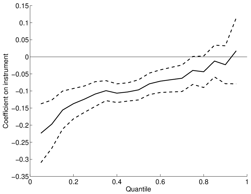
The plot shows a heterogeneous effect of the instrument on treatment—the instrument has a strong negative effect at low quantiles, but this effect decreases towards zero for higher quantiles. For quantiles from about 0.75 to 1 the instrument does not have a statistically significant effect on treatment. Even though the standard -statistic for the instrument suggests that there is no weak instrument problem (), figure 2 shows that the instrument is not uniformly strong for all counties, and indeed there are many counties (about 25% of them) where the instrument appears to have no effect at all.
Counties with smaller conditional ranks have the smallest values of —that is, the largest drops in pollution over the decade. Large drops in pollution are strongly negatively correlated with having a high baseline level of pollution in 1970 (). Consequently, the heterogeneous effect of the instrument is to be expected. Counties in nonattainment are more heavily regulated than counties in attainment. But being regulated only matters if a county has a pollution problem to begin with. Hence the counties with the highest baseline pollution are also the ones where the instrument has a strongest effect. Conversely, the counties with the lowest baseline pollution (and hence lowest potential drops in pollution) are the ones where the instrument has essentially a zero effect.
Next we implement our generalized CRC estimator. We choose two different sets of conditional ranks to consider: and . First, we omit estimating average partial effects near the tails as discussed in Section 4. Second, we omit estimating average partial effects near the region where the instrument is weak or irrelevant, as discussed in Sections 2 and 4. We split up the region for which we can estimate average partial effects into two pieces in order to examine potential heterogeneity in the effect of pollution on house prices. For each choice of we use the following tuning parameters: 1999 points for the first stage grid (equation 4), which corresponds to 1999 linear quantile regressions (an equally spaced grid with step size ). 2000 Halton draws for integration of over (equation 6). We use 500 bootstrap draws to compute 95% confidence intervals. Finally, we present a range of bandwidths from to . In our Monte Carlo simulations, the bandwidth minimized MSE for the sample size and when there was first stage heterogeneity (Table 2).
| Estimator | ||||
| OLS | 0.0861 | 0.0288 | ||
| [ 0.0079, 0.1643] | [ -0.0200, 0.0776] | |||
| TSLS | -0.4149 | -0.2073 | ||
| [ -0.7616, -0.0682] | [ -0.4258, 0.0113] | |||
| (1) | (2) | (3) | (4) | |
| Generalized CRC estimator | ||||
| -0.0241 | -0.2067 | -0.0664 | -0.1517 | |
| [ -0.3011, 0.2314] | [ -0.7879, 0.4544] | [ -0.4395, 0.1585] | [ -0.7414, 0.4363] | |
| -0.0252 | -0.1766 | -0.0640 | -0.1535 | |
| [ -0.2994, 0.2239] | [ -0.7635, 0.4540] | [ -0.3981, 0.1407] | [ -0.6894, 0.3974] | |
| -0.0261 | -0.1545 | -0.0670 | -0.1580 | |
| [ -0.2974, 0.2210] | [ -0.7419, 0.4498] | [ -0.3864, 0.1215] | [ -0.6441, 0.3634] | |
| -0.0266 | -0.1364 | -0.0703 | -0.1592 | |
| [ -0.2940, 0.2187] | [ -0.6967, 0.4410] | [ -0.3719, 0.1179] | [ -0.6258, 0.3310] | |
| -0.0258 | -0.1073 | -0.0755 | -0.1544 | |
| [ -0.2856, 0.2047] | [ -0.6551, 0.4255] | [ -0.3422, 0.1057] | [ -0.5988, 0.2751] | |
| -0.0248 | -0.0954 | -0.0784 | -0.1524 | |
| [ -0.2807, 0.2009] | [ -0.6329, 0.4430] | [ -0.3321, 0.1031] | [ -0.5927, 0.2636] | |
| Observations | 983 | 983 | ||
| County data book controls? | No | Yes | ||
| Entries show estimates of coefficients on change in TSP over 1970-1980, and corresponding 95-percent confidence intervals for several different estimators: ordinary least squares, two-stage least squares, and a variety of bandwidths for our generalized correlated random coefficient model estimator. TSP here is in units of grams/m3 rather than grams/mg/m3. Columns (1) and (3) show the generalized CRC estimates for conditional ranks over while columns (2) and (4) use . All regressions are first differenced from 1970 to 1980. The outcome variable is 1980 log-housing value minus 1970 log-housing value. The treatment variable of interest is the 1980 TSP value minus the 1970 TSP value. All controls are also first differenced. The instrument is mid-decade nonattainment status (see body text for further details). OLS and TSLS confidence intervals are computed via asymptotic plug-in estimators of the heteroskedasticity robust standard errors. The generalized CRC model confidence intervals are computed using 500 bootstrap draws. | ||||
Table 4 shows the main results. There are four columns. Columns (1) and (2) show estimation results without any control variables while columns (3) and (4) show estimation results with the control variables. Chay and Greenstone present additional specifications which use a “flexible functional form”, but they do not specify what precisely they mean, and they have not responded to our requests for clarification. Hence we present only their first two specifications. Columns (1) and (3) show the generalized CRC estimates for the choice while columns (2) and (4) show estimates for .
First, notice that OLS—which is a first-differences regression here—has the perverse sign (implying prices go up when pollution goes up), and is even statistically significant without covariates, as also found by Chay and Greenstone (their Table 3 panel C columns 1 and 2). The TSLS results also mirror the main findings of Chay and Greenstone (their Table 5 panel A columns 1 and 2): Without covariates, we find a large negative effect of pollution on log house prices: a 1 g/m3 reduction in mean TSP causes a 0.42 percent increase in property values. With covariates, this effect size is cut in half and becomes marginally statistically insignificant. Chay and Greenstone’s corresponding TSLS point estimate is with a 95 percent confidence interval of , which is not too different from the confidence interval we obtain (the difference is likely due to the data discrepancies previously mentioned).
Second, consider the bootstrap confidence intervals for the generalized CRC estimates. None of them are statistically significant. We have already seen that the instrument is strongest for smaller conditional ranks. Consequently, the confidence intervals are nearly twice as wide for the ‘weaker’ instrument region than for the ‘stronger’ instrument region . For the region , the confidence intervals are roughly the same length as for TSLS for column (3), and they’re actually smaller for column (1). But the point estimates for both of these columns are close to zero, as expected under the sorting story discussed below. Consequently, since the TSLS confidence interval was already quite close to zero, the generalized CRC estimate confidence intervals here have just been shifted over to be centered near zero.
Next consider the generalized CRC estimates. Begin by considering the point estimates. The point estimates are fairly insensitive to changes in bandwidths, especially after controlling for covariates. When controlling for covariates, the estimates for are roughly twice as large as those for . A similar finding is true when comparing column (2) to column (1), although the difference in magnitudes is much larger without the controls. Moreover, all the CRC estimates are smaller than the TSLS estimates. These findings are consistent with the possibility that households sort according to their unobserved preference for clean air during the baseline year of 1970. In that case, households with the strongest taste for clean air will move to counties with low baseline pollution, while households who do not care about clean air will move to counties with high baseline pollution. As we saw earlier, the baseline pollution and conditional rank are strongly correlated. Hence counties where the instrument has the strongest effect are also counties where most households do not care about clean air, and so we find close to zero effects for . For counties with households that moderately care about clean air, , we find moderate sized effects. For counties with households that care strongly about clean air, , we are unable to identify their preferences, since those are precisely the counties where the instrument has little or no effect—because those are the counties with little pollution to begin with. The finding that TSLS is larger than all the CRC estimates suggests that the effects for counties with are larger than , the effect we found for . This is because TSLS is a weighted average effect, where the weights depend on the strength of the instrument. Although counties in will receive close to zero weight in forming the TSLS estimand, if their actual effect size is large enough it can still pull up the overall estimate.
In this application, we showed that the instrument has a naturally interpreted heterogeneous effect due to differences in baseline pollution levels. We showed that the data is consistent with sorting, and that comparing our CRC estimates with TSLS allows us to draw conclusions about effects for counties where the instrument is weak. Overall, our findings suggest that there is substantial heterogeneity in the size of the effect of pollution on housing prices.
7 Conclusion
In this paper we have studied a linear correlated random coefficients model. We provided conditions under which we can point identify the average partial and treatment effects of an endogenous treatment variable by using variation in an instrumental variable. In contrast to previous research, these conditions allow for heterogeneous effects of the instrument in the first stage equation, as well as binary or discrete instruments in many cases. Our identification argument led directly to a simple estimator of a trimmed average of the outcome coefficients. This estimator is just an average of weighted least squares regressions, where the weights depend on a first stage estimator. We established -consistency and asymptotic normality of this estimator, and showed that it performs well in finite sample simulations. We have illustrated how allowing for and analyzing heterogeneity in the first stage and in the outcome equation can be easily and fruitfully incorporated into a typical applied instrumental variables analysis.
Several issues remain for future research. First, it may be theoretically interesting to modify our estimator to better account for boundary effects both due to kernel smoothing and first stage rank estimation. Second, we have not provided a method for choosing the bandwidth , which is an important question in practice. Third, we assumed the set for which the relevance condition I5 holds is known a priori. In some applications, this is a reasonable assumption, such as in our empirical application. In other applications, it may not be reasonable. In principle, this set can be estimated in a preliminary step, and then the previous analysis can be repeated by using this estimated set in place of . This extension is both nontrivial and of independent interest, and we leave it to future work. Fourth, it may be helpful to explore modifications of our proposed estimator to achieve efficiency gains. Finally, we are coding a Stata module that will enable practitioners to apply the estimator in this paper with minimal investment.
Appendix A Proofs
Proof of Proposition 1.
For any , and we have
where the first equality follows because for , is continuous by I2 and , the second follows by I2 and the equivariance to monotone transformations property of quantiles, the third follows because is strictly increasing by I2, and the fourth uses I4. Since the right-hand side does not depend on , we conclude that .
The second statement follows because if and only if for . Hence, conditional on , is a stochastic function of for . Since, by I3, the derived endogenous variables, , , are functions of and , they are also stochastic functions of alone after conditioning on . Thus, conditional on , is only stochastic through . Since (as implied by ), this shows that as well. ∎
Proof of Theorem 3.
We begin by rewriting the model as , where . Substituting into (5), we have with and . For any square matrix , let denote the absolute value of the smallest eigenvalue of . Then I5 and E5 imply that for some . Defining , we have , since for all .44 4 That is indeed a random variable (in the sense of being a measurable function on the underlying sample space) follows from Theorem 18.19 of Aliprantis and Border (2006) combined with standard results. Centering, integrating over and scaling by , we obtain by Lemma A.1 that
Next, define and note that our assumptions only ensure that is defined for . For we use the convention that , which will help to ease notation.55 5 The alternative would be to define and related functions (its derivatives, etc.) case by case, which seems unnecessarily tedious. Then
| (8) |
where the second equality follows by changing the variable of integration from to and the third equality follows with denoting the boundary of and denoting almost-sure equality because .66 6 Since almost-sure equality is sufficient for determining limiting distributions, we will drop the “a.s.” qualifier in the following. Note that every component of the vector is twice continuously differentiable at all , since I5 and E5 imply that is twice continuously differentiable at all (the interior of ) with first and second component-wise derivatives and , while for .77 7 The differentiability of for can be determined using the calculus rules for matrices of functions derived in Section 6.5 of Horn and Johnson (1991). For , a second order element-by-element application of Young’s form of Taylor’s Theorem yields
| (9) |
Let so that from (8) we have . Substituting the Taylor expansion in (9) into the definition of and using the symmetry of , and , we obtain
| (10) | ||||
It can be shown through some tedious algebra that I5, E5 and E6 imply that is finite. As a result, the second term in (10) is , since by E7
and by finite and E4,
Substituting the asymptotically linear form for given in E7 into the first term in (10), we obtain
| (11) |
Some tedious algebra shows that I5, E5 and E6 imply that is finite. Consequently, the second term in (11) is asymptotically negligible under E7 since
The first term in (11) can be written as a second-order V-statistic with a symmetric kernel by defining and , so that
As noted, it can be shown that is finite under our moment and smoothness assumptions. It can similarly be shown that I5, E5 and E6 imply that is also finite. These observations and E7 imply that
for both and . Since , this implies that for all and , by which we can conclude that
That is, the second-order V-statistic is asymptotically equivalent to a second-order U-statistic, see e.g. pg. 206 of Serfling (1980).88 8 Serfling’s discussion is limited to scalar-valued variables, but the modification for vector-valued variables is immediate. Recapping, we have now shown that
| (12) |
We determine the projection of the U-statistic in (12) by computing for , where the notation is shorthand for . First, since for by E1 and E7,
which has mean zero, because and by Proposition 1. Second,
where the third equality uses the law of iterated expectations (noting that is deterministic conditional on ) and the fourth equality uses and .99 9 This expression for the component-wise derivative of follows immediately from the rules in Section 6.5 of Horn and Johnson (1991). Applying the law of iterated expectations shows that , since for by E7. We have now shown that , and , so that by the central limit theorem for U-statistics (e.g. Theorem A on page 192 of Serfling 1980)1010 10 Serfling’s discussion is limited to scalar-valued variables. The original work by Hoeffding (1948) contains an explicit statement of the vector case; see also Chapter 5 of Kowalski and Tu (2008) for a modern treatment.
| (13) |
Combining equations (12) and (13) and applying Slutsky’s theorem with from Lemma A.1, we have
The result now follows after scaling both sides by . ∎
Lemma A.1.
Under the assumptions of Theorem 3, and
Proof of Lemma A.1.
Let , let denote the norm and let denote the matrix operator norm induced by the norm. Then
| (14) |
where the first inequality follows because for vector-valued function and component-wise integration we have , and the second inequality uses the sub-multiplicative property of the matrix operator norm.
First, we consider the behavior of
where with . Notice that both and are Nadaraya-Watson kernel regression estimators of the matrix with , but that the weights in use the generated regressor , while the weights in use . Recent work on nonparametric regression with generated regressors has established that under our assumptions.1111 11 In particular, we appeal to Lemma 1 of Mammen et al. (2012), but see also Sperlich (2009), Mammen et al. (2013), Hahn and Ridder (2013), Lee (2013) and Escanciano et al. (2014) for related results. We verify the conditions for Lemma 1 of Mammen et al. (2012). In their Assumption 1, (i) is E1, (ii) is satisfied with , (iii) is E5, (iv) is not used in the proof of their Lemma 1, (v) is E3 and (vi) is met under E4 and E7. Their Assumptions 2 and 3 are satisfied by our E7, while their Assumption 4 is not used in the proof of their Lemma 1. The rate of is determined by computing on pg. 1141 and observing their notational convention of leaving out terms. Using standard results in the literature, our assumptions also ensure that , with the dominant rate being given E4.1212 12 For example, see Lemma B3 of Newey (1994). Since this rate also dominates , it follows that . Note that this also implies that . Using these observations, the definition of and I5 with E5, we have that
The same rate applies to , because finite-dimensional norms are equivalent.
A rate of convergence for follows similarly after using the definition of to write
The difference of the first two terms in these expressions is uniformly again by Lemma 1 of Mammen et al. (2012).1313 13 The verification for most of their conditions is as in footnote 11. Their Assumption 1 (iii) is satisfied since each component of is twice continuously differentiable by E5. Since is bounded uniformly over by E2 and E5, the difference of the second two terms is also using the already established rate for , and hence . Also, since by Proposition 1, standard results again imply that under our assumptions. We conclude that . This establishes the claim via (14), since under E4, . ∎
References
- Aliprantis and Border (2006) Aliprantis, C. D. and K. C. Border (2006): Infinite Dimensional Analysis: A Hitchhiker’s Guide, Springer, 3 ed.
- Angrist and Imbens (1995) Angrist, J. D. and G. W. Imbens (1995): “Two-Stage Least Squares Estimation of Average Causal Effects in Models with Variable Treatment Intensity,” The Journal of the American Statistical Association, 90, 431–442.
- Angrist et al. (2010) Angrist, J. D., M. P. Keane, E. E. Leamer, A. Nevo, J.-S. Pischke, C. A. Sims, J. H. Stock, and M. D. Whinston (2010): “Symposia: Con out of Economics,” The Journal of Economic Perspectives, 24, 3–94.
- Beran and Hall (1992) Beran, R. and P. Hall (1992): “Estimating Coefficient Distributions in Random Coefficient Regressions,” The Annals of Statistics, 1970–1984.
- Blundell and Powell (2004) Blundell, R. W. and J. L. Powell (2004): “Endogeneity in Semiparametric Binary Response Models,” The Review of Economic Studies, 71, 655–679.
- Chamberlain (1992) Chamberlain, G. (1992): “Efficiency Bounds for Semiparametric Regression,” Econometrica, 60, 567–596.
- Chay and Greenstone (2005) Chay, K. Y. and M. Greenstone (2005): “Does Air Quality Matter? Evidence from the Housing Market,” The Journal of Political Economy, 113, 376–424.
- Chernozhukov et al. (2010) Chernozhukov, V., I. Fernández-Val, and A. Galichon (2010): “Quantile and Probability Curves Without Crossing,” Econometrica, 78, 1093–1125.
- Chernozhukov et al. (2011) Chernozhukov, V., I. Fernández-Val, and A. Kowalski (2011): “Quantile Regression with Censoring and Endogeneity,” Working paper.
- Chernozhukov et al. (2009) Chernozhukov, V., I. Fernández-Val, and B. Melly (2009): “Inference on Counterfactual Distributions,” Working paper.
- Chernozhukov et al. (2012) ——— (2012): “Inference on Counterfactual Distributions,” Econometrica (forthcoming).
- Chernozhukov and Hansen (2005) Chernozhukov, V. and C. Hansen (2005): “An IV Model of Quantile Treatment Effects,” Econometrica, 73, 245–261.
- Chesher (2003) Chesher, A. (2003): “Identification in Nonseparable Models,” Econometrica, 71, 1405–1441.
- Deaton et al. (2010) Deaton, A., J. J. Heckman, and G. W. Imbens (2010): “Forum on the Estimation of Treatment Effects,” The Journal of Economic Literature, 48, 356–455.
- D’Haultfœuille and Février (2012) D’Haultfœuille, X. and P. Février (2012): “Identification of Nonseparable Models with Endogeneity and Discrete Instruments,” Working paper.
- Doksum (1974) Doksum, K. (1974): “Empirical Probability Plots and Statistical Inference for Nonlinear Models in the Two-Sample Case,” The Annals of Statistics, 2, 267–277.
- Ekeland et al. (2004) Ekeland, I., J. J. Heckman, and L. Nesheim (2004): “Identification and Estimation of Hedonic Models,” The Journal of Political Economy, 112, 60.
- Escanciano et al. (2014) Escanciano, J. C., D. T. Jacho-Chavez, and A. Lewbel (2014): “Uniform Convergence of Weighted Sums of Non and Semiparametric Residuals for Estimation and Testing,” Journal of Econometrics, 178, 426–443.
- Florens et al. (2008) Florens, J. P., J. J. Heckman, C. Meghir, and E. Vytlacil (2008): “Identification of Treatment Effects Using Control Functions in Models With Continuous, Endogenous Treatment and Heterogeneous Effects,” Econometrica, 76, 1191–1206.
- Graham and Powell (2012) Graham, B. S. and J. L. Powell (2012): “Identification and Estimation of Average Partial Effects in “Irregular” Correlated Random Coefficient Panel Data Models,” Econometrica, 80, 2105–2152.
- Hahn and Ridder (2013) Hahn, J. and G. Ridder (2013): “Asymptotic Variance of Semiparametric Estimators With Generated Regressors,” Econometrica, 81, 315–340.
- Heckman and Vytlacil (1998) Heckman, J. and E. Vytlacil (1998): “Instrumental Variables Methods for the Correlated Random Coefficient Model: Estimating the Average Rate of Return to Schooling When the Return is Correlated with Schooling,” The Journal of Human Resources, 33, 974–987.
- Heckman (2001) Heckman, J. J. (2001): “Micro Data, Heterogeneity, and the Evaluation of Public Policy: Nobel Lecture,” The Journal of Political Economy, 109, 673–748.
- Heckman et al. (2010) Heckman, J. J., R. L. Matzkin, and L. Nesheim (2010): “Nonparametric Identification and Estimation of Nonadditive Hedonic Models,” Econometrica, 78, 1569–1591.
- Heckman et al. (1997) Heckman, J. J., J. Smith, and N. Clements (1997): “Making the Most Out of Programme Evaluations and Social Experiments: Accounting for Heterogeneity in Programme Impacts,” The Review of Economic Studies, 64, 487–535.
- Hoderlein et al. (2010) Hoderlein, S., J. Klemelä, and E. Mammen (2010): “Analyzing the Random Coefficient Model Nonparametrically,” Econometric Theory, 26, 804–837.
- Hoderlein and Sherman (2013) Hoderlein, S. and R. Sherman (2013): “Identification and Estimation in a Correlated Random Coefficients Binary Response Model,” Working paper.
- Hoeffding (1948) Hoeffding, W. (1948): “A Class of Statistics with Asymptotically Normal Distribution,” The Annals of Mathematical Statistics, 19, 293–325.
- Horn and Johnson (1991) Horn, R. A. and C. R. Johnson (1991): Topics in Matrix Analysis, Cambridge: Cambridge University Press.
- Imbens (2007) Imbens, G. (2007): “Nonadditive Models with Endogenous Regressors,” in Advances in Economics and Econometrics: Theory and Applications, Ninth World Congress, ed. by R. Blundell, W. Newey, and T. Persson, Cambridge University Press, New York, vol. 3.
- Imbens and Angrist (1994) Imbens, G. W. and J. D. Angrist (1994): “Identification and Estimation of Local Average Treatment Effects,” Econometrica, 62, 467–475.
- Imbens and Newey (2009) Imbens, G. W. and W. K. Newey (2009): “Identification and Estimation of Triangular Simultaneous Equations Models Without Additivity,” Econometrica, 77, 1481–1512.
- Jun (2009) Jun, S. J. (2009): “Local Structural Quantile Effects in a Model with a Nonseparable Control Variable,” Journal of Econometrics, 151, 82–97.
- Kasy (2011) Kasy, M. (2011): “Identification In Triangular Systems Using Control Functions,” Econometric Theory, 27, 663–671.
- Kasy (2013) ——— (2013): “Identification in General Triangular Systems,” Working paper.
- Koenker and Bassett (1978) Koenker, R. and G. Bassett (1978): “Regression Quantiles,” Econometrica, 46, 33–50.
- Kowalski and Tu (2008) Kowalski, J. and X. M. Tu (2008): Modern Applied U-statistics, Wiley.
- Lee (2013) Lee, Y.-Y. (2013): “Partial Mean Processes with Generated Regressors: Continuous Treatment Effects and Nonseparable Models,” Working paper.
- Li and Tobias (2011) Li, M. and J. L. Tobias (2011): “Bayesian Inference in a Correlated Random Coefficients Model: Modeling Causal Effect Heterogeneity with an Application to Heterogeneous Returns to Schooling,” Journal of Econometrics, 162, 345–361.
- Mammen et al. (2012) Mammen, E., C. Rothe, and M. Schienle (2012): “Nonparametric Regression With Nonparametrically Generated Covariates,” The Annals of Statistics, 40, 1132–1170.
- Mammen et al. (2013) ——— (2013): “Semiparametric Estimation with Generated Covariates,” Working paper.
- Masten (2012) Masten, M. A. (2012): “Random Coefficients on Endogenous Variables in Simultaneous Equations Models,” Working paper.
- Newey (1994) Newey, W. K. (1994): “Kernel Estimation of Partial Means and a General Variance Estimator,” Econometric Theory, 10, 233–253.
- Palmquist (2005) Palmquist, R. B. (2005): “Property Value Models,” Handbook of Environmental Economics, 2, 763–819.
- Powell et al. (1989) Powell, J. L., J. H. Stock, and T. M. Stoker (1989): “Semiparametric Estimation of Index Coefficients,” Econometrica, 57, 1403–1430.
- Rosen (1974) Rosen, S. (1974): “Hedonic Prices and Implicit Markets: Product Differentiation in Pure Competition,” The Journal of Political Economy, 82, 34–55.
- Rothe (2009) Rothe, C. (2009): “Semiparametric Estimation of Binary Response Models with Endogenous Regressors,” Journal of Econometrics, 153, 51–64.
- Ruppert and Wand (1994) Ruppert, D. and M. P. Wand (1994): “Multivariate Locally Weighted Least Squares Regression,” The Annals of Statistics, 22, 1346–1370.
- Serfling (1980) Serfling, R. J. (1980): Approximation Theorems of Mathematical Statistics, New York: John Wiley & Sons.
- Smith and Huang (1995) Smith, V. K. and J.-C. Huang (1995): “Can Markets Value Air Quality? A Meta-analysis of Hedonic Property Value Models,” The Journal of Political Economy, 209–227.
- Sperlich (2009) Sperlich, S. (2009): “A Note on Non-parametric Estimation with Predicted Variables,” Econometrics Journal, 12, 382–395.
- Torgovitsky (2012) Torgovitsky, A. (2012): “Identification of Nonseparable Models with General Instruments,” Working paper.
- Torgovitsky (2013) ——— (2013): “Minimum Distance from Independence Estimation of Nonseparable Instrumental Variables Models,” Working paper.
- Train (2009) Train, K. (2009): Discrete Choice Methods with Simulation, Cambridge University Press, 2 ed.
- U.S. Department of Commerce. Bureau of the Census (2008) U.S. Department of Commerce. Bureau of the Census (2008): County and City Data Book [United States], 1983. ICPSR version, Ann Arbor, MI: Inter-university Consortium for Political and Social Research (ICPSR) [distributor], http://doi.org/10.3886/ICPSR08256.v1.
- U.S. Department of Commerce. Bureau of the Census (2012) ——— (2012): County and City Data Book [United States] Consolidated File: County Data, 1947-1977, ICPSR07736-v2, Ann Arbor, MI: Inter-university Consortium for Political and Social Research (ICSPR) [distributor], http://doi.org/10.3886/ICPSR07736.v2.
- U.S. Environmental Protection Agency (2001) U.S. Environmental Protection Agency (2001): “Historical TSP data, 1970–1999,” http://www.epa.gov/ttn/airs/airsaqs/archived%20data, accessed: 10-8-2013.
- van der Vaart and Wellner (1996) van der Vaart, A. W. and J. A. Wellner (1996): Weak Convergence and Empirical Processes: With Applications to Statistics, Springer.
- Wooldridge (1997) Wooldridge, J. M. (1997): “On Two Stage Least Squares Estimation of the Average Treatment Effect in a Random Coefficient Model,” Economics Letters, 56, 129–133.
- Wooldridge (2003) ——— (2003): “Further Results on Instrumental Variables Estimation of Average Treatment Effects in the Correlated Random Coefficient Model,” Economics Letters, 79, 185–191.
- Wooldridge (2008) ——— (2008): “Instrumental Variables Estimation of the Average Treatment Effect in the Correlated Random Coefficient Model,” in Modelling and Evaluating Treatment Effects in Econometrics (Advances in Econometrics, Volume 21), ed. by D. Millimet, J. Smith, and E. Vytlacil, Emerald Group Publishing Limited, 93–116.