Transport in quenched disorder: light diffusion in strongly heterogeneous turbid media
Abstract
We present a theoretical and experimental study of light transport in disordered media with strongly heterogeneous distribution of scatterers formed via non-scattering regions. Step correlations induced by quenched disorder are found to prevent diffusivity from diverging with increasing heterogeneity scale, contrary to expectations from annealed models. Spectral diffusivity is measured for a porous ceramic where nanopores act as scatterers and macropores render their distribution heterogeneous. Results agree well with Monte Carlo simulations and a proposed analytical model.
Series of incremental random changes govern the evolution of countless systems around us, from the movement of particles and molecules [1, 2, 3, 4] and wave propagation in disordered media [5, 6], to the foraging of animals [7] and spread of disease [8]. By virtue of the central limit theorem, macroscopic evolution of such random walk processes can often be explained in terms of classical diffusion. Although therefore ubiquitous, diffusion is in each particular case determined by unique microscopic mechanisms. These mechanisms are often complex and understanding the onset and speed of diffusion is generally a challenge [9, 10, 11, 12, 13, 14]. The matter is particularly relevant to research in optics of disordered media, including the study of radiative transfer through planetary atmospheres [15, 16, 17], optical imaging and spectroscopy in biomedical [18] and material science [19] and, more recently, anomalous diffusion in engineered disordered materials [20, 21, 22, 23, 24].
Multiple scattering of light is typically viewed as a Poissonian random walk of independent and exponentially-distributed steps. This viewpoint inherently assumes a uniform random distribution of scatterers throughout the medium and results in a well-known expression for the diffusion constant [25], , where is the average transport velocity for light in the medium and the transport mean free path. This diffusivity relation, however, breaks down in systems with an heterogeneous distribution of scatterers, such as clouds, biological tissues, porous materials and foams. The reason is two-fold. First, the presence of non-scattering regions in the scattering medium leads to a broader (non-exponential) distribution of step lengths, which, in turn, induces an increase of the diffusivity [26]. Second, the quenched (i.e. spatially frozen) heterogeneity induces step correlations that tend to counteract the increase in diffusivity caused by long steps [21, 26]. Due to the complexity of these aspects, understanding of light transport in systems with heterogeneous distribution of scatterers remains rather limited. Important insight has, nonetheless, been reached with the development of generalized transport equations and homogenization theory [27, 28, 29, 30, 31, 32, 33, 34, 35] as well as probabilistic analysis of random walks [36, 37, 26]. When it comes to quenched disorder, most works are theoretical and fall within the context of anomalous diffusion [38, 39, 40, 21, 23, 24]. Experimental and theoretical investigations of how regular diffusion is affected by quenched (frozen) disorder and the accompanying step correlations are, on the other hand, largely missing.
In this Letter, we theoretically and experimentally investigate light diffusion in heterogeneous systems constituted by turbid media with embedded non-scattering regions (holes). Special focus is on how quenched disorder influence transport. The transport process, which can be referred to as a holey random walk [26], is illustrated in Fig. 1.
An analytical model for the diffusivity in such media is developed and compared to direct Monte Carlo simulations (using sphere packings to define hole arrangement). An important finding is that step correlations prevent the diffusivity to diverge with increasing heterogeneity size, contrary to expectations from annealed models. Experiments are conducted on a custom made ceramic with a bimodal pore size distribution: a nanoporous, strongly scattering base with embedded macropores acting as holes. Time-resolved measurements of light transmission allows assessment of diffusivity in the 600-900 nm spectral range, and results are found to be in agreement with theory.
The system under consideration is a turbid medium characterized by a transport mean free path and containing non-scattering spherical holes of radius at filling fraction . The holes do not overlap and may be arranged randomly or periodically. In the limit of , step correlations become negligible and an (approximate) analytical expression for the resulting diffusion constant can be calculated from the ratio of the mean squared step () to the mean step () [26]. In general, however, the resulting diffusivity is not known. As approaches and becomes smaller than (cf. Fig. 1), step correlations get increasingly important and the diffusion constant becomes difficult to assess. To gain insight into this matter, we performed a series of Monte Carlo simulations (MC) of random walks in three-dimensional systems containing randomly or periodically arranged holes with . The diffusion constant can be estimated by looking at the evolution of the mean square displacement (MSD) at long times. In the diffusive limit, the MSD is linear with time, (in 3D). Figure 2 shows the time-dependent mean square displacement (MSD) for the cases of both strong and negligible step correlations ( and , respectively). In the latter case, the transition from ballistic to diffusive transport is smooth and similar to that observed in most random walks with independent increments. In great contrast, the presence of strong step correlations results in a MSD evolution that goes from ballistic to diffusive via a transient subdiffusive behavior (cf. [21]). This behavior is caused by the fact that long steps through holes often are counteracted by steps back through the same hole and constitutes a fingerprint of step correlations in disordered media (cf. trajectories in Fig. 1).
Let us now focus on the fact that strong step correlations goes hand in hand with random walkers being likely to return to the same hole several times before reaching a new one. We propose that transport in such systems can be viewed as a random walk on a lattice (similar to the approach used to understand deterministic diffusion in a periodic Lorentz gas [41, 42]), where the holes correspond to the lattice sites, with the lattice constant and the hole-hole transfer time. The diffusivity is then simply given by [43]. The difficult part consists in determining and . We propose that (i) the lattice constant can be approximated by the lattice constant of a periodic face-centered cubic lattice, , and (ii), in the limit when the distance between voids is much larger than , the transfer time can be obtained from classical diffusion in a spherical shell with diffusivity . The analytical model as a whole is illustrated in Fig. 3. As we shall see and discuss below, although the model relies on several important approximations, it grasps the essential physics of the process and allows quantitative comparison with MC and experiments.
The transfer time is a sum of (i) the time spent on returning to the hole , (ii) the time to cross the hole when first reaching it and after returning to it, and (iii) the time spent on reaching a new hole once the return series is broken. The number of returns before transfer to a new hole follows a geometric distribution, on average being , and the number of crossings equals . We therefore reach
| (1) |
where is the average chord length ( for spheres, assuming isotropic flux) and the light velocity in the hole. Analytical expressions for the unknown parameters in Eq. 1 were derived by solving the diffusion equation in spherical shells (derivation given in Supplemental Material) and are summmarized here. and can be retrieved from Eq. 2 via and , and and from Eq. 3 via and . There, is the Jonquière’s function (the polylogarithm) [44], , is the physical thickness of the spherical shell, and the extrapolated thickness ( being the extrapolation length that can be calculated as done for light diffusion in, e.g., planar slabs [45]). The remaining step is to set the shell thickness adequately. The actual diffusive process between spherical holes being particularly complex, the derivation of an exact value for that would take into account all characteristics of the medium (hole arrangement, filling fraction, etc) seems out-of-reach. Nevertheless, setting between (smallest gap) and (distance from hole edge to center of next hole) appears reasonable and works well for the structures considered here. Above all, the exact value of has little effect on the relation between diffusivity and hole size reported below, which is a main message of the paper.
| (2) | ||||
| (3) |
Figure 4 shows how diffusivity is modified with increasing hole size (index-matched system, fixed), see note 11 1 Note that for a given hole filling fraction , the diffusivity will depend essentially on the ratio . This follows from a scaling consideration: when scaling the holey system and random walk with a factor , we have that and and . For diffusion constants, we therefore will have .. Diffusivity is reported with respect to the homogenized counterpart, i.e. the diffusion constant for a system with the same amount of scatterers but distributed homogeneously, [26]. The outcome of MC and of the analytical model presented above are given by the markers and the solid lines respectively. Clearly, the model captures the essence of the transport process (for large ). For the periodic and random holey systems, quantitative agreement occurs when setting the shell thickness to and , respectively (i.e. midway between the limits introduced above). The diffusivity enhancement evaluated from the annealed model (Ref. [26]) is also shown for comparison (dashed line). The ”annealed” diffusion constant diverges due to a diverging mean squared step length (the mean step length, remaining constant), while the ”quenched” diffusion constants saturate at a value of about 1.6-1.7 times that of the homogenized system. This leads us to a very important conclusion: In quenched disordered systems, step correlations become so strong with increasing heterogeneity size that they completely counteract the increase of , thereby preventing the diffusivity to diverge. It is interesting to realize that in a one-dimensional system, regardless of how scatterers are distributed. The average number of scatterers that needs to be passed over macroscopic distances remains the same. Clearly, the situation is very different in three-dimensional systems.
We now test this prediction experimentally. We have manufactured porous ceramics with a bimodal pore size distribution by sintering a mixture of a zirconia nano particles, latex nanoparticles and 180 m diameter PMMA microspheres. Manufacturing details are given in Supplemental Material. Briefly, latex nanoparticles and microspheres are burned out during sintering, leaving a nanoporous ceramic with embedded macropores occupying around 30% of the total volume (the porosity of the nanoporous part being 46%). The latex particles are used as spacers, increasing the final distance between the different zirconia particles and, as a result, also increasing light scattering (see Ref. [46]). The nanoporous part acts as the turbid medium, and by manufacturing a reference sample without any macropores, its can be measured. The optical properties of these materials are studied via optical time-of-flight spectroscopy [47, 48]. Short picosecond pulses are injected into the sample and the diffuse transmission is resolved in time using time-correlated single photon counting. The system used is described in detail in Refs. [49, 50] and allows coverage of the 600-900 nm spectral range. The diffusion constant (and absorption coefficient) can be determined from the temporal shape of the transmitted pulse. Using a reasonable estimate of the effective refractive index (here, we use the averaged permittivity), of the nanoporous part can be estimated from the measured of the reference sample (via with ). Accordingly, the turbid material between holes, is found to exhibit ranging from 0.7m at 600 nm to 2.2m at 900 nm and low absorption (0.026 cm-1 at 660 nm down to 0.005 cm-1 at 900 nm). The small size of the nanopores makes scattering strongly wavelength-dependent, and the transport scattering coefficient decays as (in good agreement with previous reports on scattering of nanoporous ceramics [51, 48]).
Figure 5a shows the diffusivity spectra for the holey (bimodal) system and for the nanoporous reference, and compares it to MC and the proposed analytical model. The refractive index mismatch between holes and nanoporous media is taken into account. The discrepancy between experiments and theory may be due to differences in between the reference and the holey system (scattering is very sensitive to the microstructure and differences related to the inclusion and burnout of microspheres cannot be ruled out) or to the inaccuracy in extracting from experimentally. Clearly, the holey system exhibits significantly faster diffusion than its homogenized counterpart (here , where refers to the refractive index calculated from the averaged permittivity, in an attempt to take into account the change in average refractive index that follows from removal of solid material). At the same time, due to step correlations, diffusion is slower than what could be expected from the step length distribution. This is seen in Fig. 5b, keeping in mind that if steps were uncorrelated, would diverge quickly (as in Fig. 4). The retrieved diffusivity enhancements are between 1.5 and 1.8, in agreement with our previous analysis.
Let us also note that the non-linear relation between and has an important consequence: the shape of diffusivity spectra is not only dependent on the microstructure (e.g. scatterer or pore size). This has bearing on the interpretation of diffuse spectra in general. It is, for example, common to convert diffusivity spectra into a transport scattering spectra and use that to assess particle size [52]. This procedure relies on a linear relation between and , valid for homogeneously turbid media but, as shown here, not valid for holey media. While the nanoporous reference media has a diffusivity spectra that corresponds to a decay of , the holey system – when analyzed in the same way – exhibit a decay. This change in apparent scattering spectra is induced by heterogeneity, not by an increase of pore size.
To conclude, this work provides an initial understanding and a first experimental investigation of the importance of step correlations due to quenched disorder on diffusion in strongly heterogeneous media. We have found that step correlations can counteract completely the effect of a broad step length distribution, preventing diffusivity to diverge with increasing scale of heterogeneities. This effect was predicted theoretically, and confirmed experimentally and numerically. An important implication, relevant to analytical spectroscopy in general, is that strong heterogeneity complicates assessment of microstructural characteristics based on diffusivity spectra. In addition, besides the fundamental questions brought up in this study, we expect future challenges as the topic of light diffusion in strongly heterogeneous turbid media is generalized to include, for instance, non-spherical heterogeneities and/or anisotropic holey random walks (with relevance to, e.g., anisotropic diffusion in compressed porous matter [53]).
Acknowledgements.
T.S. acknowledges funding from the Swedish Research Council (postdoctoral fellowship Grant No. 2010-887). K.V. acknowledges support by LABEX WIFI (Laboratory of Excellence within the French Program ”Investments for the Future”) under references ANR-10-LABX-24 and ANR-10-IDEX-0001-02 PSL⋆. The reported research has also received funding from the European Research Council under the European UnionÕs Seventh Framework Programme (FP7/2007-2013) ERC grant agreement number 291349, and from LASERLAB-EUROPE (grant agreement number 284464). The authors are also grateful to Erik Alerstam, Matteo Burresi and Romolo Savo for long-time collaboration and fruitful discussions.References
- [1] Brown, R. A brief account of microscopical observations made in the months of june, july and august, 1827, on the particles contained in the pollen of plants; and on the general existence of active molecules in organic and inorganic bodies. Phil. Mag. 4, 161–173 (1828).
- [2] Einstein, A. Über die von der molekularkinetischen theorie der wärme geforderte bewegung von in ruhenden flüssigkeiten suspendierten teilchen. Ann. Phys. 17, 549–560 (1905).
- [3] Berg, H. Random Walks in Biology. Princeton paperbacks (Princeton University Press, 1993).
- [4] Cussler, E. Diffusion: Mass Transfer in Fluid Systems (Cambridge University Press, 2009).
- [5] Sheng, P. Introduction to wave scattering, localization and mesoscopic phenomena. Springer series in materials science (Springer, 2006).
- [6] Akkermans, É. & Montambaux, G. Mesoscopic physics of electrons and photons (Cambridge University Press, 2007).
- [7] Viswanathan, G. The Physics of Foraging: An Introduction to Random Searches and Biological Encounters (Cambridge University Press, 2011).
- [8] Brockmann, D., Hufnagel, L. & Geisel, T. The scaling laws of human travel. Nature 439, 462–465 (2006).
- [9] Bouchaud, J.-P. & Georges, A. Anomalous diffusion in disordered media: Statistical mechanisms, models and physical applications. Phys. Rep. 195, 127–293 (1990).
- [10] Elaloufi, R., Carminati, R. & Greffet, J.-J. Diffusive-to-ballistic transition in dynamic light transmission through thin scattering slabs: a radiative transfer approach. J. Opt. Soc. Am. A 21, 1430–1437 (2004).
- [11] Lukić, B., Jeney, S., Tischer, C., Kulik, A. J., Forró, L. & Florin, E.-L. Direct observation of nondiffusive motion of a Brownian particle. Phys. Rev. Lett. 95, 160601 (2005).
- [12] Huang, R., Chavez, I., Taute, K. M., Lukic, B., Jeney, S., Raizen, M. G. & Florin, E.-L. Direct observation of the full transition from ballistic to diffusive Brownian motion in a liquid. Nat. Phys. 7, 576–580 (2011).
- [13] Novikov, D. S., Fieremans, E., Jensen, J. H. & Helpern, J. A. Random walks with barriers. Nat. Phys. 7, 508–514 (2011).
- [14] Wang, B., Kuo, J., Bae, S. C. & Granick, S. When Brownian diffusion is not Gaussian. Nat. Mater. 11, 481–485 (2012).
- [15] Chandrasekhar, S. Radiative transfer. Dover Books on Physics (Dover Publications, 1960).
- [16] Hansen, J. E. & Travis, L. D. Light scattering in planetary atmospheres. Space Sci. Rev. 16, 527–610 (1974).
- [17] Davis, A. B. & Marshak, A. Solar radiation transport in the cloudy atmosphere: a 3D perspective on observations and climate impacts. Rep. Prog. Phys. 73, 026801 (2010).
- [18] Welch, A. J. & Gemert, M. J. C. Optical-Thermal Response of Laser-Irradiated Tissue (Springer, 2010).
- [19] Berne, B. J. & Pecora, R. Dynamic Light Scattering: With Applications to Chemistry, Biology, and Physics (Dover Publications, 2000).
- [20] Barthelemy, P., Bertolotti, J. & Wiersma, D. S. A Lévy flight for light. Nature 453, 495–498 (2008).
- [21] Barthelemy, P., Bertolotti, J., Vynck, K., Lepri, S. & Wiersma, D. S. Role of quenching on superdiffusive transport in two-dimensional random media. Phys. Rev. E 82, 011101 (2010).
- [22] Vynck, K., Bertolotti, J., Barthelemy, P. & Wiersma, D. S. Superdiffusion of light in Lévy glasses in ”Optical Properties of Photonic Structures: Interplay of order and disorder” (Taylor & Francis, 2012).
- [23] Buonsante, P., Burioni, R. & Vezzani, A. Transport and scaling in quenched two- and three-dimensional Lévy quasicrystals. Phys. Rev. E 84, 021105 (2011).
- [24] Groth, C. W., Akhmerov, A. R. & Beenakker, C. W. J. Transmission probability through a Lévy glass and comparison with a Lévy walk. Phys. Rev. E 85, 021138 (2012).
- [25] van Rossum, M. C. W. & Nieuwenhuizen, T. M. Multiple scattering of classical waves: microscopy, mesoscopy, and diffusion. Rev. Mod. Phys. 71, 313–371 (1999).
- [26] Svensson, T., Vynck, K., Grisi, M., Savo, R., Burresi, M. & Wiersma, D. S. Holey random walks: Optics of heterogeneous turbid composites. Phys. Rev. E 87, 022120– (2013).
- [27] Davis, A. & Marshak, A. Fractal Frontiers, chap. Lévy kinetics in slab geometry: scaling of transmission probability, 63–72 (World Scientific, Singapore, 1997).
- [28] Kostinski, A. B. On the extinction of radiation by a homogeneous but spatially correlated random medium. J. Opt. Soc. Am. A 18, 1929–1933 (2001).
- [29] Bal, G. Particle transport through scattering regions with clear layers and inclusions. J. Comput. Phys. 180, 659–685 (2002).
- [30] Davis, A. B. & Marshak, A. Photon propagation in heterogeneous optical media with spatial correlations: enhanced mean-free-paths and wider-than-exponential free-path distributions. J. Quant. Spectrosc. Radiat. Transfer 84, 3–34 (2004).
- [31] Scholl, T., Pfeilsticker, K., Davis, A. B., Klein Baltink, H., Crewell, S., Löhnert, U., Simmer, C., Meywerk, J. & Quante, M. Path length distributions for solar photons under cloudy skies: Comparison of measured first and second moments with predictions from classical and anomalous diffusion theories. J. Geophys. Res. 111, D12211 (2006).
- [32] Frank, M. & Goudon, T. On a generalized Boltzmann equation for non-classical particle transport. Kinet. Relat. Models 3, 395–407 (2010).
- [33] Davis, A. B. & Mineev-Weinstein, M. B. Radiation propagation in random media: From positive to negative correlations in high-frequency fluctuations. J. Quant. Spectrosc. Radiat. Transfer 112, 632–645 (2011).
- [34] Larsen, E. W. & Vasques, R. A generalized linear boltzmann equation for non-classical particle transport. J. Quant. Spectrosc. Radiat. Transfer 112, 619–631 (2011).
- [35] Lovejoy, S., Watson, B., Grosdidier, Y. & Schertzer, D. Scattering in thick multifractal clouds, part ii: Multiple scattering. Physica A 388, 3711–3727 (2009).
- [36] Behrens, D. J. The effect of holes in a reacting material on the passage of neutrons. Proc. Phys. Soc. A 62, 607–616 (1949).
- [37] Lieberoth, J. & Stojadinović, A. Neutron streaming in pebble beds. Nucl. Sci. Eng. 76, 336–344 (1980).
- [38] Fogedby, H. C. Lévy flights in random environments. Phys. Rev. Lett. 73, 2517–2520 (1994).
- [39] Schulz, M. Lévy flights in a quenched jump length field: a real space renormalization group approach. Phys. Lett. A 298, 105–108 (2002).
- [40] Burioni, R., Caniparoli, L., Lepri, S. & Vezzani, A. Lévy-type diffusion on one-dimensional directed Cantor graphs. Phys. Rev. E 81, 011127 (2010).
- [41] Machta, J. & Zwanzig, R. Diffusion in a periodic lorentz gas. Phys. Rev. Lett. 50, 1959– (1983).
- [42] Klages, R. & Dellago, C. Density-dependent diffusion in the periodic lorentz gas. J. Stat. Phys. 101, 145–159 (2000).
- [43] ben Avraham, D. & Havlin, S. Diffusion and reactions in fractals and disordered systems (Cambridge University Press, 2000).
- [44] Jonquière, A. Note sur la série ’, vol. 17, p. 142-152 (1889). B. Soc. Math. Fr. 17, 142–152 (1889).
- [45] Contini, D., Martelli, F. & Zaccanti, G. Photon migration through a turbid slab described by a model based on diffusion approximation: I. Theory. Appl. Opt. 36, 4587–4599 (1997).
- [46] Svensson, T., Adolfsson, E., Burresi, M., Savo, R., Xu, C., Wiersma, D. S. & Svanberg, S. Pore size assessment based on wall collision broadening of spectral lines of confined gas: experiments on strongly scattering nanoporous ceramics with fine-tuned pore sizes. Appl. Phys. B 110, 147–154 (2013).
- [47] Patterson, M., Chance, B. & Wilson, B. Time resolved reflectance and transmittance for the noninvasive measurement of tissue optical-properties. Appl. Opt. 28, 2331–2336 (1989).
- [48] Svensson, T., Adolfsson, E., Lewander, M., Xu, C. T. & Svanberg, S. Disordered, strongly scattering porous materials as miniature multipass gas cells. Phys. Rev. Lett. 107, 143901 (2011).
- [49] Bassi, A., Farina, A., D’Andrea, C., Pifferi, A., Valentini, G. & Cubeddu, R. Portable, large-bandwidth time-resolved system for diffuse optical spectroscopy. Opt. Express 15, 14482–14487 (2007).
- [50] Bargigia, I., Tosi, A., Shehata, A. B., Frera, A. D., Farina, A., Bassi, A., Taroni, P., Mora, A. D., Zappa, F., Cubeddu, R. & Pifferi, A. Time-resolved diffuse optical spectroscopy up to 1700 nm by means of a time-gated InGaAs/InP single-photon avalanche diode. Appl. Spectrosc. 66, 944–950 (2012).
- [51] Svensson, T. & Shen, Z. Laser spectroscopy of gas confined in nanoporous materials. Appl. Phys. Lett. 96, 021107 (2010).
- [52] Mourant, J., Fuselier, T., Boyer, J., Johnson, T. & Bigio, I. Predictions and measurements of scattering and absorption over broad wavelength ranges in tissue phantoms. Appl. Opt. 36, 949–957 (1997).
- [53] Alerstam, E. & Svensson, T. Observation of anisotropic diffusion of light in compacted granular porous materials. Phys. Rev. E 85, 040301 (2012).
- [54] Note that for a given hole filling fraction , the diffusivity will depend essentially on the ratio . This follows from a scaling consideration: when scaling the holey system and random walk with a factor , we have that and and . For diffusion constants, we therefore will have .
I SUPPLEMENTAL MATERIAL
II I. Diffusion through spherical shells
Here, we derive an analytical expression for the energy density in diffusive spherical shells by solving the diffusion equation in spherical coordinates with Dirichlet boundary conditions and a Dirac delta impulse as an initial condition. Based on this, we derive expressions for time-resolved reflection and transmission. The theoretical results are compared with direct Monte Carlo simulations of transport in spherical shells. It should be noted that the notation used here differs from the notation used in the main article. In the main article refers to the radius of holes while it here refers to the spherical coordinate.
II.1 The diffusion equation
Conside a spherical shell of inner radius and outer radius containing a diffusive medium with diffusion constant . A spherical plane source is placed at in order to have rotational invariance.

The diffusion equation in its general form is written as
| (4) |
We impose the Dirichlet boundary conditions and , where and take the initial condition .
In spherical coordinates, the Laplacian operator can be written as
| (5) |
and the energy density can be written by separating the variables as to construct separable solutions of the diffusion equation. Since we assume rotational invariance, the angular terms disappear in the Laplacian and the energy density can then be written simply as
| (6) |
and the diffusion equation in spherical coordinates, after division on each side by , reads
| (7) |
where is the separation constant. The solution of the temporal equation simply gives , such that . At this point, the equation that remains to be solved is
| (8) |
We can use the known solution of the spherical Bessel differential equation:
| (9) |
with the eigenvalue order generally associated with the spherical harmonics. The solution of the equation is written in terms of spherical Bessel functions as:
| (10) |
where and are two constants depending on the boundary conditions, and and are the spherical Bessel functions of the first and second kind, respectively, of order . Due to rotational invariance in our case, only the order remains. Interestingly, the spherical bessel functions of order 0 can be written as elementary functions: and . The solution of our equation can then be written as:
| (11) |
II.2 Boundary conditions
We now apply the Dirichlet boundary conditions and . By applying the former, we find that , such that
| (12) |
and by applying the latter, we arrive at the following condition: . Writing leads to the condition that should be a multiple of . Thus, the eigenvalues should be:
| (13) |
with .
Since the eigenfunctions are complete on a bounded domain, the fundamental solution can be written as an eigenfunction series as , in which the constant is contained within the coefficients . We therefore have
| (14) |
II.3 Initial conditions
We now turn to the determination of the coefficients , uniquely prescribed by the initial conditions at and are given by the usual orthogonality formula:
| (15) |
with the integration volume. With , we are left with two volume integrals to solve:
| (16) |
The volume element in spherical coordinates and rotational invariance becomes . The volume integral of the numerator is simply the function and the denominator can be evaluated exactly. After some maths, we find:
| (17) |
II.4 Propagator (energy density)
Equations (14,17) provide the complete solution for the propagator in diffusive spherical shells, which, all in all, simplifies to:
| (18) |
For the application of Eq. (18) to real samples, one should consider the fact that the intensity is not zero exactly at the boundary but at a distance , called the extrapolation length, where is the mean free path in the diffusive medium and is the internal reflection coefficient at the boundary. See [45] for a description on how to calculate the extrapolation length for a given mismatch in refractive index. It is possible to use Eq. (18) directly by taking the thickness as the extrapolated thickness , where is the physical thickness. Similarly, the inner radius should be taken as an extrapolated inner radius . Thus, a point source placed one mean free path apart from this boundary should be placed at .
The energy density in the spherical shell at different times is shown in Fig. 7 for a system with m, m, m and m2/ps. The source is placed at m.
II.5 Energy flux
To calculate the fluxes in transmission or reflection through the slab, it is necessary to apply the first Fick’s law of diffusion:
| (19) |
In spherical coordinates with rotational invariance, we have that . Thus, the diffusion flux can easily be calculated by spatial derivation of in Eq. (18). We find:
| (20) |
II.6 Time-resolved transmission and reflection
The time-resolved reflection and transmission are then found by integrating the fluxes over the surface of the corresponding boundaries and normalizing by the source :
| (21) |
The normalization can be verified.
II.7 Mean first-passage time
An important step is the calculation of the mean reflection and transmission (or first passage) time. This can be calculated as and , respectively. An analytical expression can be found for this quantity by using the definition of the polylogarithm, or Jonquière’s function [44], defined as , and Euler’s formula on the sine and cosines. One finds (Eq. 2 in the main text):
| (22) |
In the practical example considered above, we find ps and ps.
II.8 Total transmitted/reflected flux
Similarly, the integrated transmission or reflection at position , can be expressed in terms of polylogarithms, as (Eq. 3 in main text):
| (23) | |||||
which gives, in the practical example, and .
II.9 Comparison with Monte Carlo simulations
The validity of our theoretical findings have been checked via Monte Carlo simulations of random walks in spherical shells. In these simulations, random walkers are launched one mean free path away from the inner boundary of the spherical shell (inside the spherical shell). Thereafter random walkers take isotropic, independent and exponentially distributed steps with average length . Letting the numerical example from above serve as an example, we set to 1 m and the walker velocity to m/ps (resulting in a diffusion constant of m2/ps). The MC estimates of reflection and transmission and their respective characteristic times are shown in Table 1 below along with the theoretical values presented above.
| Parameter | Theoretical value | MC estimate |
|---|---|---|
| (%) | 95.14 | 95.040.02 |
| (ps) | 0.834 | 0.8530.002 |
| (%) | 4.86 | 4.960.02 |
| (ps) | 25.661 | 25.78 0.07 |
Clearly, the theoretical values are in very good agreement with simulation outcome. Also the shapes of the time-resolved reflection and transmission agree well, as shown in Figure 8 below. Of course, more elaborate investigations of the validity of the diffusion model for, e.g., non-zero boundary conditions (mismatch in refractive index) and thin shells – extensively studied for common geometries such as slabs or semi-infinite media – remains to be done.
III II. Ceramics Manufacturing
An aqueous suspension with a solids loading of 50vol% of ZrO2 (TZ3YSE, Tosoh, Japan) and 0.3wt% of dispersant (Dolapix PC 75, Zschimmer-Schwarz, Germany) was prepared by ball milling with milling media of zirconia. The suspension was diluted with water to a solids loading of 25vol% and 6vol% of latex as binder was introduced in form of a latex emulsion (LDM 7651S, Celanese, Sweden) with a particle size of 150 nm. For the holey ceramic, polyethylene microspheres (Cospheric, USA) with a size of 180m were added to the suspension. To avoid segregation of the polyethylene microspheres in the aqueous suspension, xanthan gum (Rhodophol 23, Rhodia) was used as a thickener to increase the viscosity of the suspension. For the holey ceramic, the volume of polyethylene microspheres used corresponded to 45 vol% with respect to the total solid volume of zirconia and polyethylene microspheres. To maintain the homogeneity of the suspension with zirconia particles, latex emulsion and polyethylene micro spheres, the suspension was frozen drop by drop in liquid nitrogen followed by a freeze drying procedure to remove the ice by sublimation. The freeze dried particles were used to prepare ceramic green bodies by compaction. When the green bodies were sintered at 900∘C for two hours in a SiC furnace (Entech, Sweden), the organic additives were removed. Furthermore, the temperature was sufficient for an initial solid state diffusion, which allowed neck formation between the zirconia particles. At the same time, the temperature was not high enough to cause any sintering shrinkage of the powder compact. In this manner, a nanoporous ceramic with embedded macropores was obtained. As a reference, a material without any microsphere were also manufactured (same manufacturing procedure).
Density measurements, performed with ArchimedesÕ method, showed that the nanoporous reference has a porosity of around 46%. The holey ceramic, on the other hand, has a porosity of about 63.5%. This is in good agreement with what is expected from the added fraction of microspheres. The 45vol% microspheres should, when the other 55vol% solids has formed a nanoporous media with 46% porosity, give rise to a macroporosity of around 30% and an overall porosity (macropores and nanoporosity) of about 63%.
IV III. Optical time-of-flight experiments
The system used for experiments is depicted in Fig. 9 and has been described in detail in [49, 50]. It consists of a supercontinuum source (SuperK Extreme, NKT) emitting mode-locked laser pulses in the range 450-1750 nm at a repetition rate of 20 MHz. The white light exiting the source is dispersed by an SF10 Pellin-Broca prism and then focused on a variable slit by a 150 mm focal length achromatic doublet for spectral bandwidth selection. Tuning is achieved by the rotation of the prism. The slit plane is imaged on a 50 m graded index fiber by means of two achromatic lenses. The spectral bandwidth of the system ranges from about 3 nm at 600 nm to 6 nm at 900 nm. Light is delivered to and collected from the sample by means of 1 mm step-index fibers. The detector consists of a Hybrid PMT (HPM-100-50, Becker and Hickl, Germany). The instrumental response function (IRF), measured by setting the detection and injection fibers face-to-face, has a full-width half-maximum (FWHM) of about 180 ps over the whole spectral range. The time-of-flight (TOF) distribution of detected photons is measured by a time-correlated single photon counting (TCSPC) board (SPC-130, Becker and Hickl, Germany) mounted on the PC, which controls both the prism rotation and the data acquisition.
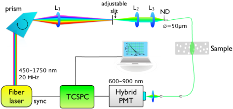
The porous ceramics was measured in transmittance geometry with co-linear fiber optics. TOF distributions was acquired in 600-900 nm range 600-900 nm (in steps of 20 nm) at an intensity that gave about 400000 counts/s. The samples were around 3 mm thick, resulting in average TOF of a few nanoseconds, depending on the wavelength (e.g. TOF curves are far wider than the IRF). The size of the optical fiber collecting transmitted light was taken into account during evaluation of TOF distribution (i.e. during the assessment of the diffusion constant).