跳到论文正文
W Papers独立论文阅读器 arXiv:1310.6340 论文正文 计算阅读时间 · 0%
引用这篇论文根据当前论文元数据生成,正式投稿前建议核对。


License: CC BY 3.0
arXiv:1310.6340v2 [physics.acc-ph] 13 Apr 2015

A Novel Spin-Light Polarimeter
for the
Electron Ion Collider

prajwal mohanmurthy

[Uncaptioned image]

Honors Undergraduate Thesis

Submitted in partial fulfillment of the requirements for the award of the degree of

Bachelor of Science in Physics [Honors]
Department of Physics and Astronomy

Mississippi State University, MS, USA

Nov 25, 2012

1. Reviewer: Dr. Dipangkar Dutta

2. Reviewer: Dr. Seth Oppenheimer

3. Reviewer: Dr. Paul Reimer

Day of the defense: Dec 04, 2012

Prajwal Mohanmurthy: A Novel Spin-Light Polarimeter for the Electron Ion Collider, Honors Undergraduate Thesis , © Nov 25, 2012

To,

Amma and Appa,

for their dedication and admirable way of life.

Foreword

††margin: [i]eRHIC: High Energy Electron-Ion collider, http://www.bnl.gov/cad/eRhic/, Retrieved on: Nov 25, 2011 ††margin: [i]eRHIC: High Energy Electron-Ion collider, http://www.bnl.gov/cad/eRhic/, Retrieved on: Nov 25, 2011 ††margin: [ii]ELIC: Electron Light Ion Collider at CEBAF, http://casa.jlab.org/research/elic/elic.shtml, Retrieved on: Nov 25, 2011 ††margin: [ii]ELIC: Electron Light Ion Collider at CEBAF, http://casa.jlab.org/research/elic/elic.shtml, Retrieved on: Nov 25, 2011

  With Jefferson National Accelerator Facility’s (JLAB) 12​G​e​V12GeV program in construction phase with a comprehensive set of experiments already planned for the next decade, it is time to think of newer facilities that will further push the boundaries and continue the mission of a premier nuclear physics laboratory to explore the frontiers of fundamental symmetries and nature of nuclear matter. Building of an Electron Ion Collider (EIC) seems to be a natural future step. JLAB is a fixed target laboratory, but at the EIC, the target will also be accelerated thereby providing access to precision physics of quarks and gluons at much higher energies (than 12​G​e​V12GeV). JLAB mainly consists of the Continuous Electron Beam Accelerator and 33 halls where the fixed target experiments are performed. Brookhaven mainly consists of the Relativistic Heavy Ion Collider with a number of main collision points on the beam line. There have been two leading proposals for the EIC, i.e.

  • •

    eRHIC : Electron - Relativistic Electron Collider @ Brookhaven National Laboratory, Upton, NY [i]

    [Uncaptioned image]
  • •

    ELIC : Electron - Light Ion Collider @ Jefferson National Accelerator Laboratory, Newport News, VA [ii]

    [Uncaptioned image]

Brookhaven already has an ion accelerator and the eRHIC would need addition of an electron accelerator, whereas JLAB already has the electron accelerator and the ELIC would need addition of an ion accelerator.

At JLAB, polarization of the electron beam has played a vital role a number of experiments such as the PVDIS (Parity Violating Deep Inelastic Scattering) and the QWeak (which measured the weak charge of proton). To measure the polarization of the electron beam, JLAB has commissioned Compton and Møller polarimeters which have met the precision demands of JLAB, but the Møller Polarimeter generates a large background as it uses e​eee scattering to measure the polarization. The future demands greater precision in the measurement of polarization of the beam and so at the EIC, it would be convenient to have a second non-invasive polarimeter, besides a Compton Polarimeter, for systematics comparison.

Abstract

  A novel precision polarimeter will go a long way in satisfying the requirements of the precision experiments being planned for a future facility such as the Electron Ion Collider. A polarimeter based on the asymmetry in the spacial distribution of the spin light component of synchrotron radiation will make for a fine addition to the existing-conventional Møller and Compton polarimeters. The spin light polarimeter consists of a set of wriggler magnet along the beam that generate synchrotron radiation. The spacial distribution of synchrotron radiation will be measured by an ionization chamber after being collimated. The up-down spacial asymmetry in the transverse plane is used to quantify the polarization of the beam. As a part of the design process, firstly, a rough calculation was drawn out to establish the validity of such an idea. Secondly, the fringe fields of the wriggler magnet was simulated using a 2-D magnetic field simulation toolkit called Poisson Superfish, which is maintained by Los Alamos National Laboratory. This was used to account for beam motion effects and the corresponding correlations were show to be negligible. Lastly, a full fledged GEANT-4 simulation was built to study the response time of the ionization chamber. This GEANT-4 simulation was analyzed for variety of effects that may hinder precision polarimetry. It was found that a Spin-Light Polarimeter would be a fine relative polarimeter.

Acknowledgements

This work has been generously supported by Jefferson Science Associates, LLC - Undergraduate Fellowship Program at Thomas Jefferson National Accelerator Facility, VA, USA.

Additional, but substantial, funding has been provided by the Mississippi State Consortium, MS, USA, and the Office of Research & Economic Development, MS, USA. Travel funds has also been provided by the Shackouls Honors College, MS, USA, The Conference Experience for Undergraduates program of the American Physical Society’s Division of Nuclear Physics, USA, and the Graduate School of Mississippi State University, MS, USA.

Thanks are due to the Department of Physics and Astronomy at Mississippi State University, MS, USA for providing office & lab space and also the computational infrastructure required for this computational intensive work.

It would have been impossible to quickly adapt the GEANT4 code to the latest standards without the express support from Edward ’Jed‘ Legget, a graduate student in the Medium Energy Physics Group at Mississippi State University, MS, USA.

The author would also like to extend his gratitude to the Hall-A Compton group at Jefferson Lab, VA, USA, especially Dr. Gregg Franklin of Carnegie Mellon University, PA, USA for providing the basic Hall-A Compton chicane magnets’ LANL Poisson codes.

Most importantly, thanks are due to Dr. Dipangkar Dutta, who has been relentlessly at work on this project, guiding and helping the effort at every step as the major advisor and supervisor in charge.

Last, but not least, the author likes to thank the thesis defense committee members Dr. Paul Reimer of Argonne National Laboratory, IL, USA and Dr. Seth Oppenheimer of the Shackouls Honors College, MS, USA for their very thoughtful inputs.

ection]chapter

Part I   Ground Work

††margin: 1 Theory

1 Classical SR-Power Law

††margin: [1]Proposal to the EIC R & D:
https://wiki.bnl.gov/conferences/images/7/74/RD2012-11_Dutta_eic_polarimetry.pdf
††margin: [1]Proposal to the EIC R & D:
https://wiki.bnl.gov/conferences/images/7/74/RD2012-11_Dutta_eic_polarimetry.pdf
††margin: [2]D. D. Ivanenko, I. Pomeranchuk, Ya Zh. Eksp. Teor. Fiz. 16, 370 (1946); J. Schwinger, Phys. Rev. 75, 1912 (1947) ††margin: [2]D. D. Ivanenko, I. Pomeranchuk, Ya Zh. Eksp. Teor. Fiz. 16, 370 (1946); J. Schwinger, Phys. Rev. 75, 1912 (1947)
Refer to caption
Figure 1: Angular distribution of synchrotron radiation shown for the bottom half of the electron’s orbital plane. The left figure is for slow electrons, β∼0\beta\sim 0 and the right figure is for highly relativistic electrons, β∼1\beta\sim 1. [1]
††margin: [3]I. M. Ternov and V. A. Bordovitsyn, Vestn. Mosk. Univ. Ser. Fiz. Astr. 24, 69 (1983); V. A. Bordovitsyn and V. V. Telushkin, Nucl. Inst. and Meth. B266, 3708 (2008) ††margin: [3]I. M. Ternov and V. A. Bordovitsyn, Vestn. Mosk. Univ. Ser. Fiz. Astr. 24, 69 (1983); V. A. Bordovitsyn and V. V. Telushkin, Nucl. Inst. and Meth. B266, 3708 (2008)

The total radiative power due to circularly accelerated particles is given by Larmor formula which is Pc​l​a​s=23​e2​γ4​cR2P_{clas}=\frac{2}{3}\frac{e^{2}\gamma^{4}c}{R^{2}} (i.e. PP is proportional to E4E^{4}) {here Pc​l​a​sP_{clas} is the classical total radiative power, ee is the electron charge, γ=Eme​c2\gamma=\frac{E}{m_{e}c^{2}} : the Lorentz boost, cc is the speed of light, and RR is the radius of trajectory of the electrons}. The angular dependence of radiative power can also be computed via classical electromagnetism.

d​Pc​l​a​sd​Ω=e2​γ4​c4​π​R2​(1−β​C​o​s​θ)2−(1−β2)​S​i​n2​θ​C​o​s2​ϕ(1−β​C​o​s​θ)5\frac{dP_{clas}}{d\Omega}=\frac{e^{2}\gamma^{4}c}{4\pi R^{2}}\frac{(1-\beta Cos\theta)^{2}-(1-\beta^{2})Sin^{2}\theta Cos^{2}\phi}{(1-\beta Cos\theta)^{5}} (1)

In classical electrodynamics the angular distribution of radiative power from synchrotron (SR) light can be calculated, as indicated in the above eq.(1) [2] {where d​Ω=d​θ​d​ϕ\mathrm{d}\Omega=\mathrm{d}\theta\mathrm{d}\phi, and β=s​p​e​e​d​o​f​p​a​r​t​i​c​l​es​p​e​e​d​o​f​l​i​g​h​t\beta=\frac{speedofparticle}{speedoflight}}. The SR light-cone is spread over a well defined cone with the angular spread - θ\theta in retarded time Δ​t′≈Δ​θωo\Delta t^{\prime}\approx\frac{\Delta\theta}{\omega_{o}} {where ωo\omega_{o} is the angular frequency of the photon}. There is no reason to believe that the SR spectrum is mono-energetic. The spectral width of SR radiation can be formulated: Δ​ω≈1Δ​t′​(1−β)=12​γ3​ωo\Delta\omega\approx\frac{1}{\Delta t^{\prime}(1-\beta)}=\frac{1}{2\gamma^{3}\omega_{o}}. A critical acceleration can be envisioned at which the SR may consist of just 11 photon by solving the equation γ​me​c2=ℏ​ωC\gamma m_{e}c^{2}=\hbar\omega_{C}. To achieve this acceleration, a critical uniform magnetic field can be applied on an electron which is Bc=me2​c3e​ℏB_{c}=\frac{m_{e}^{2}c^{3}}{e\hbar} {here mem_{e} refers to the rest mass of an electron}. The energy of the electron at these accelerations can be called the critical energy, EC=me​c2​me​Rcℏ≈103​T​e​VE_{C}=m_{e}c^{2}\sqrt{\frac{m_{e}R_{c}}{\hbar}}\approx 10^{3}TeV for RcR_{c} of about 10​m10m. It is important to note that even though accelerated electron is under consideration, the equations above don’t have acceleration terms. This is because a conventional circular motion is used to calculate the parameters and only the speed is important as the acceleration is a function of speed.

2 Quantum Corrections

In the classical theory, the spin does not explicitly appear in the equation. But, in QED, the angular dependence of synchrotron (SR) light can be calculated to a great degree of precision and the spin of the electron involved in SR emission appears explicitly in the power law [3]. The quantum power law for SR was worked out by Sokolov, Ternov and Klepikov as a solution to the Dirac equation [4] ††margin: [4] A. A. Sokolov, N. P. Klepikov and I. M. Ternov, JETF 23, 632 (1952). ††margin: [4] A. A. Sokolov, N. P. Klepikov and I. M. Ternov, JETF 23, 632 (1952). and includes the effects introduced by electrons undergoing j→j′j\rightarrow j^{\prime} (spin dependence) transitions besides also elaborating on the fluctuations to the electron orbit (n→n′n\rightarrow n^{\prime} transitions - linear correction to orbit and s→s′s\rightarrow s^{\prime} transitions - quadratic correction to orbit). ††margin: [5] A. A. Sokolov and I. .M. Ternov, Radiation from Relativistic Electrons, A.I.P. Translation Series, New York (1986) ;
I. M. Ternov, Physics - Uspekhi 38, 409 (1995).
††margin: [5] A. A. Sokolov and I. .M. Ternov, Radiation from Relativistic Electrons, A.I.P. Translation Series, New York (1986) ;
I. M. Ternov, Physics - Uspekhi 38, 409 (1995).
The power law when integrated over all polarizations and (spacial) angular dependencies, can be written as [5];

P=PC​l​a​s​9​316​π​∑s∫0∞y​d​y(1+ξ​y)4​Is​s′2​(x)​F​(y)P=P_{Clas}\frac{9\sqrt{3}}{16\pi}\displaystyle\sum\limits_{s}\int_{0}^{\infty}\frac{y\mathrm{d}y}{(1+\xi y)^{4}}I_{ss^{\prime}}^{2}(x)F(y) (2)
F⁡(y)=1+j​j′2​[2​(1+ξ​y)​∫y∞K53​(x)​𝑑x+12​ξ2​y2​K23​(y)−j⁡(2+ξ​y)​ξ​y​K13​(y)]+1−j​j′2​ξ2​y2​[K23​(y)+l​K13​(y)]F(y)=\frac{1+jj^{\prime}}{2}\Big[2(1+\xi y)\int_{y}^{\infty}K_{\frac{5}{3}}(x)\mathrm{d}x+\frac{1}{2}\xi^{2}y^{2}K_{\frac{2}{3}}(y)-j(2+\xi y)\xi yK_{\frac{1}{3}}(y)\Big]\\ +\frac{1-jj^{\prime}}{2}\xi^{2}y^{2}\Big[K_{\frac{2}{3}}(y)+lK_{\frac{1}{3}}(y)\Big] (3)

{Where ξ=3​B2​Bc​γ\xi=\frac{3B}{2B_{c}}\gamma, ’jj’ is the spin of the electron, y=ωoωcy=\frac{\omega_{o}}{\omega_{c}}, x=34​ξ​γ3​y2(1+ξ​y)2x=\frac{3}{4}\frac{\xi\gamma^{3}y^{2}}{(1+\xi y)^{2}}, Is​s′​(x)I_{ss^{\prime}}(x) are Laguerre functions, and Kn​(x)K_{n}(x) are modified Bessel functions}.

If ξ<<1\xi<<1 (given Bc≈4.41×10⁹B_{c}\approx 4.41\times 10^{9} Tesla) then Eq. (3) can be Taylor expanded in terms of powers of ξ\xi as follows;

P=Pc​l​a​s[(1−55​324ξ+643ξ2)−(1+j​j′2)(jξ+59ξ2+245​348jξ2)+(1−j​j′2)(43ξ2+315​3432jξ2)+…]P=P_{clas}\Big[\left(1-\frac{55\sqrt{3}}{24}\xi+\frac{64}{3}\xi^{2}\right)-\left(\frac{1+jj^{\prime}}{2})(j\xi+\frac{5}{9}\xi^{2}+\frac{245\sqrt{3}}{48}j\xi^{2}\right)\\ +\left(\frac{1-jj^{\prime}}{2}\right)\left(\frac{4}{3}\xi^{2}+\frac{315\sqrt{3}}{432}j\xi^{2}\right)+...\Big] (4)

Eq. (3) and (4) include the a number of effects;

  • •

    Classical SR

  • •

    Thomas Precession

  • •

    Larmor Precession

  • •

    Interference between Larmor and Thomas Precession

  • •

    Radiation from intrinsic magnetic moment (including anomalous magnetic moment)

Eq. (4) can be re-expressed as a difference between power from unpolarized and polarized electron beam.

PS​p​i​n=PP​o​l.−PU​n​P​o​l.=−jξPC​l​a​s∫0∞9​38​πy2K13(y)dyP_{Spin}=P_{Pol.}-P_{UnPol.}=-j\xi P_{Clas}\int_{0}^{\infty}\frac{9\sqrt{3}}{8\pi}y^{2}K_{\frac{1}{3}}(y)\mathrm{d}y (5)

Eq. (5) is essentially the spin light that this project is based on which opens up the possibility of using SR part to measure the polarization of the beam.

The power law in eq. (5), that was derived using QED, has been extensively tested and verified at the Novosibirsk Storage ring over a large range of wavelengths (of SR). For this, the Novosibirsk group used a "snake" shaped wiggler magnet to produce the SR from a relatively low energy electron beam of about 0.5​G​e​V​@​100​μ​A0.5GeV@100\mu A. ††margin: [5] S. A. Belomesthnykh et al., Nucl. Inst. and Meth. 227, 173 (1984). ††margin: [5] S. A. Belomesthnykh et al., Nucl. Inst. and Meth. 227, 173 (1984).

Refer to caption
Figure 2: Magnetic snake used at the VEPP-4 as a source of SR to test the spin dependence of SR. [6]
Refer to caption
Figure 3: Results from the experiment showing the increase in intensity of SR as the polarization builds up and then suddenly drops to zero when an RF field is used to depolarize the beam. [6]
††margin: [6] K. Sato, J. of Synchrotron Rad., 8, 378 (2001). ††margin: [6] K. Sato, J. of Synchrotron Rad., 8, 378 (2001).

Figure 3, clearly demonstrated the power dependence of the SR on beam-electron polarization. It remains to be shows as to how the SR spectra could be measured.

The spin flip probability has a special significance in modern day electron storage rings and is given by the relation [4];

W↑⁣↓=1τ​(1+j​8​315)W_{\uparrow\downarrow}=\frac{1}{\tau}(1+j\frac{8\sqrt{3}}{15}) (6)
††margin: [7] J. Le Duff, P. C. Marin, J. L. Manson, and M. Sommev, Orsay - Rapport Technique, 4-73 (1973). ††margin: [7] J. Le Duff, P. C. Marin, J. L. Manson, and M. Sommev, Orsay - Rapport Technique, 4-73 (1973).

{where j=+1j=+1 is spin along the magnetic field (and j=−1j=-1 is spin against magnetic field), and τ\tau is the time involved in the process}.

As a result of the probability of spin aligning with the magnetic field direction would become very high over long periods of time. A circulating electron beam, such as ones in storage rings self polarize, and this has been studied in great detail at many storage rings such as ones at DESY, PSI and CESR though it was first observed at the Orsay storage ring [7].

3 Spin - Light

  In the Spin-Light polarimeter, the spin-flip term in the power law does not play an important role. The integral power law without the spin-flip term can be written as [4];

Pγ=9​ηe16​π3c​e2R2γ5∫0infy2​d​y(1+ξ​y)4∮dΩ(1+α2)2×[K232​(z)+α21+α2​K132​(z)+j​ξ​y​α1+α2​K13​(z)​K23​(z)]P_{\gamma}=\frac{9\eta_{e}}{16\pi^{3}}\frac{ce^{2}}{R^{2}}\gamma^{5}\int_{0}^{\inf}\frac{y^{2}\mathrm{d}y}{(1+\xi y)^{4}}\oint\mathrm{d}\Omega(1+\alpha^{2})^{2}\times\\ \Big[K^{2}_{\frac{2}{3}}(z)+\frac{\alpha^{2}}{1+\alpha^{2}}K^{2}_{\frac{1}{3}}(z)+j\xi y\frac{\alpha}{\sqrt{1+\alpha^{2}}}K_{\frac{1}{3}}(z)K_{\frac{2}{3}}(z)\Big] (7)

where z=ω2​ωC​(1+α2)23z=\frac{\omega}{2\omega_{C}}(1+\alpha^{2})^{\frac{2}{3}} and α=γ​ψ\alpha=\gamma\psi where ψ\psi is the vertical angle i.e. above and below the orbit of the electron. Notice that the last term with a jj disappears from the integral over all angles (−π2≤ψ≤π2-\frac{\pi}{2}\leq\psi\leq\frac{\pi}{2}). But for an electron that is polarized, the power below (i.e. −π2≤ψ≤0-\frac{\pi}{2}\leq\psi\leq 0 and above (i.e. −π2≤ψ≤π2-\frac{\pi}{2}\leq\psi\leq\frac{\pi}{2}) are spin dependent. More importantly the difference between the power radiated above and power radiated below is directly spin dependent, which can be directly obtained from Eq. (7) in differential form for circular arcs in the circular cross-section the SR-light cone at an angle θ\theta.

Δ​Pγ​(j)Δ​θ=32ℏ​c​γ3​yR×3π2​1137​Iee​j​ξ​γ​∫y1y2y2​𝑑y​∫0αα​(1+α2)32​K13​(z)​K23​(z)​𝑑α\frac{\Delta P_{\gamma}(j)}{\Delta\theta}=\frac{3}{2}\frac{\hbar c\gamma^{3}y}{R}\times\\ \frac{3}{\pi^{2}}\frac{1}{137}\frac{I_{e}}{e}j\xi\gamma\int_{y_{1}}^{y_{2}}y^{2}\mathrm{d}y\int_{0}^{\alpha}\alpha(1+\alpha^{2})^{\frac{3}{2}}K_{\frac{1}{3}}(z)K_{\frac{2}{3}}(z)\mathrm{d}\alpha (8)

††margin: 2 Initial Design

  It is obvious now that our setup will have a wiggler magnet which shall be the source of SR and an ionization chamber to measure the power spectra of the SR emitted at the wiggler magnet by the polarized electrons.

4 Wiggler Magnet

  In order to create a fan of SR light (as illustrated in Figure 5), the electron beam could be made to bend in presence of a magnet. An arrangement that would lead to the production of the SR-Cone must look similar to the "snake" magnets that were used by VEPP-4 as described in Chapter 1.

Refer to caption
Figure 4: A 3-pole wiggler with central dipole twice the length of end dipoles.

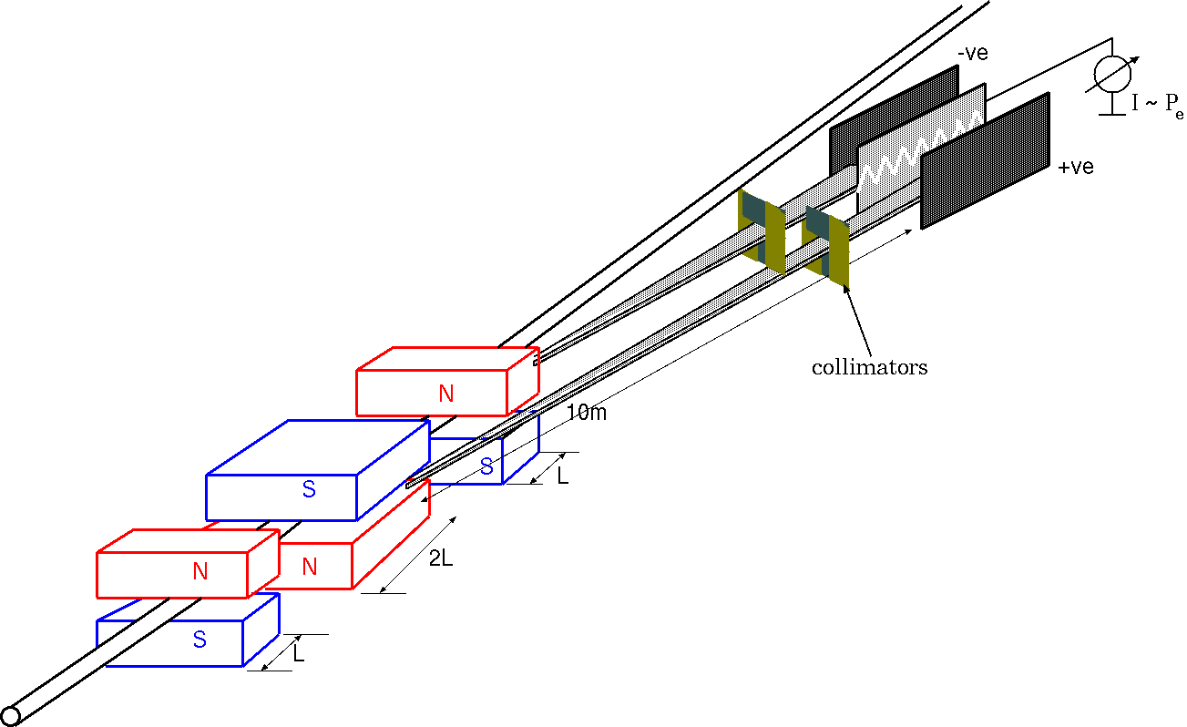
A set of 3 dipoles (3 - pole dipole), each with constant uniform magnetic field would be ideal for this purpose. The central dipole would have twice the pole length as compared to the ones on either side of the central dipole, but with a magnetic field an opposite polarity like in Figure 4. This design will give rise to 4 fans, 2 towards either side of the beam (left and right). Each of the fan will have spacial asymmetry as a function of spin - polarization of the electrons in the vertical plane (up - down the electron beam’s orbit which is perpendicular to the plane which contains the 4 fans). The 4 fans help characterize the systematics better since this configuration will flip the sign of the spin - dependent term in Eq. (8) twice essentially returning the sign to the original status.

With this geometry in mind, one could then simulate and calculate the requisite pole strengths and pole lengths appropriate to energies at Electron Ion Collider (EIC). Of course, one would also have to consider time scales at which the statistics would be sufficient to achieve the design requirement (<1%<1\%) of precision. A number of techniques were employed to tackle the above issues. Including issues such as optimizing the distance between each pole were solved through a full fledged GEANT-4 simulation.

5 Collimator

Refer to caption
Figure 5: A rough schematic of the 44 fans that shall be created by the Wiggler Magnet

The 44 fans of SR-Light need not be separated from each other. They may in fact overlap and extracting the power - asymmetry information from complicated overlappings would require extensive modeling. This might also introduce new sources of uncertainties. Therefore to uniquely sample each fan at the ionization chamber, collimators would need to be placed on each face of the dipoles to direct and separate the fans of SR. The position of the collimators will be calculated using optimized values of pole - strengths, pole - lengths and relative position of each of the dipoles.

6 Ionization Chambers

The Ionization Chambers (IC), one on each side (22 fans per IC) of the beam, could be used for measuring the spacial asymmetry in the SR - fans to be used to compute the polarization of the electrons in the beam. One would not expect a large asymmetry in the Spin-Light component (of the order of about 10−410^{-4}), therefore a high resolution, low noise IC is demanded. The IC will be very close to the beam line and the spin-independent background may be as high as 1012​p​h​o​t​o​n​s/s10^{12}photons/s, therefore the ICs have to be radiation hard. The geometry of the magnets could be changed to deal with SR Spectra with characteristic energy peak in the ranges of about 500​k​e​V−2.5​M​e​V\penalty\ 500keV-2.5MeV. ††margin: [8] A. E. Bolotnikov and B. Ramsey, Nucl. Inst. and Meth. A396, 360 (1997). ††margin: [8] A. E. Bolotnikov and B. Ramsey, Nucl. Inst. and Meth. A396, 360 (1997). An IC with Xenon as ionization media operated in the current mode can in principle handle high fluxes and have low noise disturbances [8]. It might be important to note that the Spin-Light asymmetry is spread over the entire spectra of the SR. ††margin: [9] T. Doke, Portugal Phys. 12, 9 (1981). ††margin: [9] T. Doke, Portugal Phys. 12, 9 (1981). ††margin: [10] V. V. Dmitrenko et al., Sov. Phys.-tech. Phys. 28, 1440 (1983); A. E. Bolotnikov et al., Sov. Phys.-Tech. Phys. 33, 449 (1988) ††margin: [10] V. V. Dmitrenko et al., Sov. Phys.-tech. Phys. 28, 1440 (1983); A. E. Bolotnikov et al., Sov. Phys.-Tech. Phys. 33, 449 (1988) ††margin: [11] C. Levin et al., Nucl. Inst. and Meth. A332, 206 (1993). ††margin: [11] C. Levin et al., Nucl. Inst. and Meth. A332, 206 (1993). ††margin: [12] G. Tepper and J. Losee, Nucl. Inst. and Meth. A356, 339 (1995). ††margin: [12] G. Tepper and J. Losee, Nucl. Inst. and Meth. A356, 339 (1995). ††margin: [13] A. E. Bolotnikov and B. Ramsey, Nucl. Inst. and Meth. A383, 619 (1996). ††margin: [13] A. E. Bolotnikov and B. Ramsey, Nucl. Inst. and Meth. A383, 619 (1996). ††margin: [14] G. Tepper and J. Losee, Nucl. Inst. and Meth. A368, 862 (1996). ††margin: [14] G. Tepper and J. Losee, Nucl. Inst. and Meth. A368, 862 (1996). ††margin: [15] Proportional Technologies Inc., www.proportionaltech.com. ††margin: [15] Proportional Technologies Inc., www.proportionaltech.com. Sampling radiation over large energy spectrum becomes important. Since Xenon has the lowest ionization energy of about 21.9​e​V21.9eV, among non-radioactive nobel gases, it seems to be an ideal candidate. ICs with Xenon under high pressures have already been developed and well tested to perform well in the energy ranges of 50​k​e​V−2.0​M​e​V50keV-2.0MeV [9]. Pressures involved in HPXe ICs exceed 50​a​t​m​@​0.55​g/c​c50atm@0.55g/cc but they work well at room - temperature [10],[11],[12]. One of the bottlenecks was the precision of purity of the Xenon gas in its pristine form. But owing to advances in gas purification techniques [13], a best energy resolution of 2.4%2.4\% at about 0.662​M​e​V0.662MeV has been shown to be possible when current signals from the shower is used in presence of prompt Xenon scintillation [14]. The results from this attempt has been fairly promising (Figure 6). ICs with 3%−4%3\%-4\% energy resolution are even being sold commercially by Proportional Technologies Inc. [15].

Refer to caption
Figure 6: C​s137Cs^{137}: Ei=1.7​k​V/c​mE_{i}=1.7kV/cm, pulse height spectrum in 57​a​t​m57atm at 295​K295K of xenon, Ei=1.7​k​V/c​mE_{i}=1.7kV/cm [14].

Part II   Project Work

††margin: 3 Design Considerations

7 Spin - Light Characteristics

Refer to caption
Figure 7: A. Plot of difference between the number of SR and spin light photons that go above and below the orbit of the electron (Δ​Pγ\Delta P_{\gamma}) vs. their energy
B. Plot of total number of SR, spin light photons PγP_{\gamma} vs. their energy
C. Plot of the Asymmetry vs. the photon energies
D. Plot of time required to achieve 1%1\% statistics by sampling one wavelength of the spin-light spectra vs. the energy of the photons.

The spin - dependence of the SR can be studied by examining Eq. (6-8) in Chapter 1. Using Ie=100​μ​AI_{e}=100\mu A and Ee=11​G​e​VE_{e}=11GeV, Eq. (6-8) were numerically integrated (Appendix B.1) between −1<α<1-1<\alpha<1 and Δ​θ=10​m​r​a​d\Delta\theta=10mrad , for a uniform magnetic field of B=4​TB=4T assuming 100%100\% longitudinal polarization.

In Figure 7, the total number of SR and spin light (PγP_{\gamma}) photons radiated is plotted. Also in Figure 7, is a plot the difference between the power of spin light spectra above and below the orbit of the electron (Δ​Pγ\Delta P_{\gamma}). An asymmetry term is defined to be A=Δ​PγPγA=\frac{\Delta P_{\gamma}}{P_{\gamma}}, which was used to nail down the range of energies of the photons which must be measured. Lastly, a plot of sampling time required (Ts=Δ​AA=1A​2​P​EeT_{s}=\frac{\Delta A}{A}=\frac{1}{A\sqrt{2PE_{e}}}) to achieve the design precision goals.

It immediately becomes clear that the ionization chamber, which is envisioned to measure the asymmetry (that in turn will be used to compute the electron polarization), will have to be operational at wavelengths corresponding to hard - XRays. Furthermore, the asymmetry plot, Figure 7.D, demands that the sampling be done at the higher energies (and not close to 0.5​M​e​V0.5MeV) since at higher energies the asymmetry is not rapidly changing, thus making it an ideal high-energy polarimetry technique. It might be important to note that the asymmetry is fairly low but since the integrated power of spin-light is very high, the time required for achieving 1%1\% polarimetry is only of the order of a few seconds. Also, one could plot the asymmetry and SR spectra for different energies to study the trends with change in beam energy. This indicates that there are no suppression effects at higher energies that might hinder effective polarimetry.

Refer to caption
Figure 8: (Left) A. Plot of spin light spectra over photon energies for various electron beam energies ranging from 4​G​e​V−12​G​e​V4GeV-12GeV;
(Right) B. Plot of asymmetry over photon energies for various electron beam energies ranging from 4​G​e​V−12​G​e​V4GeV-12GeV

8 Wiggler Magnet

Refer to caption
Figure 9: (Left - Right)
A. Plot of total number of spin light photons PγP_{\gamma} vs. their energy for various pole strengths
B. Plot of the newly defined term - Asymmetry vs. the photon energies for various pole strengths

In order to establish the dimensions of the dipoles, the same graphs as in Section 3.1 Figure 8 were plotted for various pole lengths and magnetic fields. First, the asymmetry increases very slowly with field strength as shown in Figure 9, and the figure of merit (time for 1%1\% statistics) improves very slowly with magnetic fields above 3​T3T as shown in Figure 10B, therefore B=4​TB=4T was chosen since 4​T4T wiggler magnets are easily available at light sources around the world. Secondly, an appropriate pole length of Lp=10​c​mL_{p}=10cm was selected by looking at Figure 10 and selecting out the pole length for the pole strength of 4​T​e​s​l​a4Tesla. It is noteworthy to see that the plot of pole length as a function of pole strength was done keeping in mind an SR fan - angular spread of about 10​m​r​a​d10mrad. The plot in Figure 10.B also re-assures the reasonable time requirement to achieve the design precision goal of 1%1\%. The last parameter in the wiggler to be fixed is the distance between each dipole.

Refer to caption
Figure 10: (Left - Right)
A. Pole length required for a 10​m​r​a​d10mrad angular spread of SR light fans with B=4​TB=4T
B. Dependence of time required to achieve 1%1\% statistics by sampling one wavelength of the spin-light spectra with pole strengths.
8.1 Effects of wiggler on the beam
††margin: [16] B. Norum, CEBAF Technical note, TN-0019 (1985). ††margin: [16] B. Norum, CEBAF Technical note, TN-0019 (1985). ††margin: [17] M. Sands, SLAC Technical note, SLAC-121 (1970). ††margin: [17] M. Sands, SLAC Technical note, SLAC-121 (1970).

A polarimeter must be non - invasive and therefore answering the question of what would be the effects of putting such as polarimeter on a beam line is very important. But the effect of a high energy electron beam emitting SR has been well studied [16]. The number of photons (NN) emitted by an electron when it is deviated by a radian, from its initial linear trajectory, when acted upon by a magnetic field is distributed as per the conventional Poisson distribution [17] about a mean value of nn;

N¯​(n)=nN​e−nN!\bar{N}(n)=\frac{n^{N}e^{-n}}{N!}\\ (9)
n⁡(Ee)=52​3​γ137=20.6​Een(E_{e})=\frac{5}{2\sqrt{3}}\frac{\gamma}{137}=20.6E_{e} (10)

The average energy of the SR photons can also be written down as {where EeE_{e} is the electron energy};

E¯e=ℏ​ω¯=32​ℏ​c​γ3R=32​ℏ​Ee3R​me3​c5\bar{E}_{e}=\hbar\bar{\omega}=\frac{3}{2}\frac{\hbar c\gamma^{3}}{R}=\frac{3}{2}\frac{\hbar E_{e}^{3}}{Rm_{e}^{3}c^{5}} (11)

In the case of a spin-light polarimeter, the beam energy is about 11​G​e​V11GeV and we choose pole strength to be about 4​T4T in Section 3.2. An angular bend of about 10​m​r​a​d10mrad of the beam is sufficient for such a polarimeter. Using the values of average number of photons emitted and their average energy, the average energy fluctuation (Δ​E¯e\Delta\bar{E}_{e}) of the beam can be computed.

n=20.62×11G​e​V×.01r​a​d=2.06n=20.62\times 11_{GeV}\times.01_{rad}=2.06 (12)
E¯e=32​ℏ​(11G​e​V)310m​me​c5=.199​M​e​V\bar{E}_{e}=\frac{3}{2}\frac{\hbar(11_{GeV})^{3}}{10_{m}m_{e}c^{5}}=.199MeV (13)
Δ​E¯eEe=n​E¯eEe≈2.5×10⁻⁵\frac{\Delta\bar{E}_{e}}{E_{e}}=\frac{\sqrt{n}\bar{E}_{e}}{E_{e}}\approx 2.5\times 10^{-5} (14)

The energy fluctuations are smaller than the typical precision with which the energy can be measured at an electron accelerator.

Another parameter which needs to be checked before proceeding, is the transverse kicks (Δ​θe\Delta\theta_{e}) received by the electrons when emitting SR photons in the magnets. The transverse kicks can be calculated in terms of angles knowing that the SR power spectrum usually peaks at an angle θγ=1γ\theta_{\gamma}=\frac{1}{\gamma} [17] {where EγE_{\gamma} is the SR - photon energy};

Δ​θe=Eγ​S​i​n​(θγ)Ee≈11.3×10⁻⁹​Ee(G​e​V)R(m)\Delta\theta_{e}=\frac{E_{\gamma}Sin(\theta_{\gamma})}{E_{e}}\approx 11.3\times 10^{-9}\frac{E_{e_{(GeV)}}}{R_{(}m)} (15)
θ¯e=n​Δ​θe≈1.5×10(r​a​d)−8\bar{\theta}_{e}=\sqrt{n}\Delta\theta_{e}\approx 1.5\times 10^{-8}_{(rad)} (16)

It can be clearly seen from Eq. (14) and Eq. (16) that both energy fluctuation and angular kicks shall be negligible. This can be seen for all practical purposes in the GEANT-4 simulation that this work demands. This polarimetry method remains a non-invasive procedure.

8.2 Effects of realistic dipole magnetic field with fringes
Refer to caption
Figure 11: Schematic diagram of the planes at which position the simulation was carried out.
Refer to caption
Figure 12: Field map of the dipole face at the center of the dipole.
Refer to caption
Figure 13: Plot of both the xx and yy components of the magnetic field on the transverse plane at the the center of the dipole (Beam pipe is centered around 1515cm mark along the ’x’ axis).
Refer to caption
Figure 14: Field map of the dipole face at the edge of the dipole.
Refer to caption
Figure 15: Plot of both the xx and yy components of the magnetic field on the transverse plane at the the edge of the dipole (Beam pipe is centered around 1515cm mark along the ’x’ axis).
††margin: [18] Poisson SuperFish 2D EM Solver, laacg1.lanl.gov/laacg/services/sfu_04_04_03.phtml,2007. ††margin: [18] Poisson SuperFish 2D EM Solver, laacg1.lanl.gov/laacg/services/sfu_04_04_03.phtml,2007.

In Section 3.2, while plotting the power spectra and the asymmetry generated by the code in Appendix B.1 a uniform field was used. But the code can also take a field map. A field map can be generated by solving Maxwell’s equations with appropriate boundary conditions. This is essential since field in the transverse plane (perpendicular to the motion of electrons) might distort the SR spectrum and thereby change the asymmetry. In fact there is a custom built suite of programs written by Los Alamos National Laboratory to precisely do this called LANL Poisson SuperFish [18].

In LANL SuperFish, the magnet geometry can be easily defined as is done in Appendix B.2. The field map of the magnet can then be plotted. Here, the field map at the edge where the electron beam enters the magnet and at the center of the dipole is presented. In Figures 11 & 13, note that the beam pipe is going at the center below the magnet pole. In Figure 13, the physical taper of the cores can be notices, since it is at the edge of the magnet face. This taper of the poles is absent in Figure 11, since it is at the center. In Figures 11 & 13, the singularities seen are the areas where the current cuts the plane. Also, it is important to note that the entire ’C’ magnet is not visible in the field-map, only the top half of the C magnet is shown in the field map.

Refer to caption
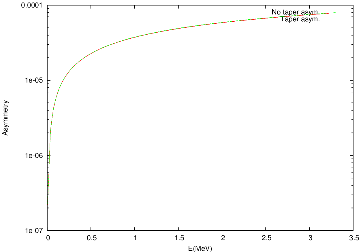
Figure 16: Plot showing the SR - Light (TotEvents_ramp) and Spin - Light (SpinLightEvents_ramp) power spectra with a realistic taper for the dipoles (Power spectra for uniform magnetic field have also been presented as _noramp).
Refer to caption
Figure 17: Plot of the assymetry with a realistic taper for the dipoles (Taper asym.).

X - Axis is to the right and left of the beam and Y - Axis is to the above and below the beam. Also the XY plane is perpendicular to the direction of motion of electron. In Figure 13, it might be important to note that there is no component of the magnetic field. This is because it is at the center of the dipole and there is no fringing of the field. But in Figure 15, there is a non - zero X component to the magnetic field since it is on the plane at the face of the magnet. A 2D simulation is sufficient since any components along the motion of electrons (Z Axis) will not affect the electrons.

The field map obtained here can be inserted into the numerical integration code (in Appendix B.1) and the power spectra and the asymmetry can be obtained. Even though there is a reduction in the total power output of light by introducing a realistic taper for dipole fields, the asymmetry has not changed. This implies that the changes introduces by the realistic dipoles are minimal.

9 Collimation and Spin-Light fan size

  Even though the distance between the 3 dipoles should in theory not affect the physics involved, it is nevertheless an essential design parameter. A reasonable value of about 1​m1m distance between each dipole was used to start with but this value will be definitely fixed with a full fledged GEANT-4 simulation. A fan with 10​m​r​a​d10mrad spread would then give rise to a spot which is 10​c​m10cm big in the horizontal plane, 10​m10m from the wiggler where the ionization chambers will be placed. A more important dimension of the SR-spot at the ionization chamber is its height in the vertical direction. An angular spread of Δ​θ=1/γ=100​μ​r​a​d\Delta\theta=1/\gamma=100\mu rad would then give rise to a spot which is 1​m​m1mm big in the horizontal plane, 10​m10m from the wiggler, where the ionization chambers will be placed.

Refer to caption
Figure 18: A schematic diagram showing the 4 fans of SR that originate at the wiggler magnet system.
Refer to caption
Figure 19: A schematic diagram showing the Spin-Light profile at the Ionization Chamber
Refer to caption
Figure 20: A schematic diagram showing the 4 fans of SR that originate at the wiggler magnet system with collimators.
Refer to caption
Figure 21: A schematic diagram showing the Spin-Light profile at the Ionization Chamber with collimators.

Figure 18 shows the origin of 4 different fans of SR Light (which contain the spin-light component) that are being created at the wiggler magnet. Corresponding fans of SR light create 4 spots at the ionization chamber which is located 10​m10m from the wiggler magnet system. The spots at the ionization chamber as shown in Figure 19, merge with each other and may destroy the spacial asymmetry that contains the polarization information. Therefore collimators may be employed at the face of every dipole to select out a small section of the bigger SR fan as illustrated in Figure 20. After collimation the spots are all uniquely separated and 4 distinct spots can be observed at the ionization chamber (as in Figure 21).

10 Ionization Chambers

  The Spin Light polarimeter detector would consist of a position sensitive ionization chamber to measure the up-down asymmetry in the SR - Light. Such a position sensitive detector that could charecterize X-Ray spectrum has already been developed at the Advanced Light Source, Argonne National Laboratory and at Sprin-8 Light Source. This uses a split - plane which essentially divides the ionization chamber into 22 separate chambers but with a common electrode. These have been demonstrated to have a resolution of about 5​μ​m5\mu m [19]. Subtracting the currents from the top chamber from the bottom chamber will then give a measure of the asymmetry in the SR-Light. A schematic diagram of the protoype is presented in Figure 23. ††margin: [19] K. Sato, J. of Synchrotron Rad., 8, 378 (2001); T. Gog, D. M. Casa and I. Kuzmenko, CMC- CAT technical report. ††margin: [19] K. Sato, J. of Synchrotron Rad., 8, 378 (2001); T. Gog, D. M. Casa and I. Kuzmenko, CMC- CAT technical report.

Refer to caption
Figure 22: A schematic diagram of a prototype split plate Ionization Chamber.

  Using such an ionization chamber, one could easily carryout relative polarimetry. A more challenging but possible option would be to have an absolute polarimeter.

10.1 Relative Polarimetry
††margin: [20] G. Tepper and J. Losee, Nucl. Inst. and Meth. A356, 339 (1995). ††margin: [20] G. Tepper and J. Losee, Nucl. Inst. and Meth. A356, 339 (1995).

  A Xenon media split plate would be an ideal differential ionization chamber. Using T​iTi windows of sufficient size could in principle cut down on low energy X-Rays (<50​K​e​V<50KeV) and T​iTi has been shown to have a high transparency for hard X-Ray [20]. A schematic diagram of the ionization chambers for the Spin-Light polarimeter is presented in Figure 23. The Spin-Light Polarimeter Ionization chamber shall have 22 compartments into which the 22 collimated fans of SR Light will enter. On each side of the electron beam is one split - plane ionization chamber and therefore all 44 fans of SR - Light, produced at the wiggler magnet, are measured at the 22 ionization chambers. Notice for polarimetry, just one ionization chamber is required. The 22 separate ICs will provide abundant statistics in a short time.

Refer to caption
Figure 23: A schematic diagram of the Spin - Light Polarimeter Ionization Chamber.
Refer to caption
Figure 24: A schematic diagram of signal collection configuration.

The signal which will give us a measure of the spacial asymmetry could be measured by subtracting the currents from the UP and DOWN parts of the chamber after being amplified as shown in Figure 24. The spin - light asymmetry shall be of opposite signs on the LEFT and RIGHT parts of the chamber, since SR fans from adjacent wiggler dipole (which have opposite polarity) enter one on each side of the chamber (L-R). Beam motion effects are nullified as any motion will have have trend (same sign) on both the LEFT and RIGHT sides of the chambers. Each half (T-B) of the split plane collector measures a current proportional to the difference of photon flux between the 22 sides and therefore any vertical beam motion effects cancel out to the first order. The two signals indicated in Figure 24 can be quantified. This definitely shows that the vertical beam motion effects will be canceled out to first order.

S1=NS​Rl+Ns​p​i​nl+Δ​Nzl−(NS​Rr−Ns​p​i​nr+Δ​Nzr)=2​Ns​p​i​nS_{1}=N^{l}_{SR}+N^{l}_{spin}+\Delta N^{l}_{z}-(N^{r}_{SR}-N^{r}_{spin}+\Delta N^{r}_{z})=2N_{spin} (17)
S2=NS​Rl−Ns​p​i​nl−Δ​Nzl−(NS​Rr+Ns​p​i​nr−Δ​Nzr)=−2​Ns​p​i​nS_{2}=N^{l}_{SR}-N^{l}_{spin}-\Delta N^{l}_{z}-(N^{r}_{SR}+N^{r}_{spin}-\Delta N^{r}_{z})=-2N_{spin} (18)
††margin: [21] G. Tepper and J. Losee, Nucl. Inst. and Meth. A356, 339 (1995). ††margin: [21] G. Tepper and J. Losee, Nucl. Inst. and Meth. A356, 339 (1995).

{Where NS​Rl⁡(r)N^{l(r)}_{SR} is the number of SR Photons on the left (right) side of the middle split plate, Ns​p​i​nl⁡(r)N^{l(r)}_{spin} is the number of spin-light photons and Δ​Nzl⁡(r)\Delta N^{l(r)}_{z} is the difference in number of photons introduced by the vertical beam motion}.

Hence S1−S2=4​Ns​p​i​nS_{1}-S_{2}=4N_{spin} is a measure of longitudinal polarization and S1+S2S_{1}+S_{2} will give a measure of transverse polarization. The ability to measure both transverse and longitudinal polarization makes this a powerful polarimetry technique. The number of photons absorbed in the ionization chamber can be computed by multipling the SR Power equation Eq.(8) with the absorption function (where μ\mu is the absorption coefficient which is material specific and tt is the length of the chamber) A⁡(λ,t)=1−e−μ⁡(λ).tA(\lambda,t)=1-e^{-\mu(\lambda).t}. With the help of values of μ\mu obtained from NIST database [21], a plot of photons absorbed in a ionization chamber that is 50​c​m50cm in length and held at 1​a​t​m1atm pressure is shown in Figure 25. The spectra of number of photons absorbed was used to then calculate the detector response which in this case is asymmetry weighted against absorption.

Refer to caption
Figure 25: NIST plot of dependence of absorption coefficient of Xenon on the photon energy [21].
Refer to caption
Figure 26: Plot of photons absorption spectra for the ionization chamber.
Refer to caption
Figure 27: Schematic diagram of the entire Differential Spin Light Polarimeter (The only visible difference between the absolute and relative polarimeters in the schematics is the difference in collector plate bias).
10.2 Absolute Polarimetry
Refer to caption
Figure 28: Schematic diagram of the entire Absolute Spin Light Polarimeter (The only visible difference between the absolute and relative polarimeters in the schematics is the difference in collector plate bias).
††margin: [22]S. Kubota, M. Suzuki and J, Ruan, Phys. Rev. B 21, 2632 (1980). ††margin: [22]S. Kubota, M. Suzuki and J, Ruan, Phys. Rev. B 21, 2632 (1980).

A relative polarimeter could be turned into an absolute polarimeter by making a few modifications to the ionization chamber. for absolute polarimeter, a high resolution ionization chamber is required and so the natural choice would be a high pressure Xenon IC. A cylindrical chamber capable of withstanding 50​a​t​m50atm of pressure could house the IC setup whereas the rest of the structure would remain unchanged from the relative IC with a few additions. The electrodes could be held in place with thin walled B​e​OBeO ceramic material which would provide uniform electric field and reduce acoustic noise while being transparent to hard XRays [21]. This design eliminates the need for field guide rings which require additional feed throughs and internal voltage dividers. In order to shield against space charge build-up, a wire mesh grid should be placed near the anode which carries a voltage that is intermediate in value to the drift potential (potential between the anode and the cathode). The ratio of the grid field to drift field can be adjusted to maximize the shielding efficiency. The cathodes and the intermediate grids would be build from stainless steel wire mesh to allow the compressed xenon UV scintillation light to be collected by the UV sensitive photomultiplier tubes (PMT). The scintillation signal has a fast component with a decay time of 2.2​n​s2.2ns and slow component with a decay time of 27​n​s27ns [22]. The scintillation light can be used during calibration, to provide a time zero reference for ionization position determination and can also be used for background suppression using pulse shape discrimination and for anti-coincidence Compton suppression. This will help improve the energy resolution and hence aid the determination of the sensitive energy range of the chamber (during calibration, when the chamber is operated in charge mode). Similar HPXe chamber (without the split anode) have been successfully operated [21] for over a decade now and are also commercially available. A schematic for such an IC is shown in Figure 29. The readout electronics chain would consist of a pre-amplifier and shaping amplifier unlike the current amplifiers used in the current mode ICs. In addition, one would also have to establish the linearity of such an IC given the high flux of photons making the calibration of the IC very challenging.

Refer to caption
Figure 29: A schematic diagram of the Absolute Spin - Light Polarimeter Ionization Chamber.

The vertical beam motion effects in an absolute IC shall be cancelled to the first order just like in the differential IC. The current signal from each chamber is an integral over the sensitive energy range of the chamber. This energy range convoluted with the detector response function, can be determined by calibrating the chamber at low electron beam currents (∼1​n​A\sim 1nA), where the photon flux is low enough to operate the chambers in charge mode. The pulse height spectrum from these calibration runs can be used to determine the sensitive energy range and the detector response function. The uncertainty in determining the absolute value of the range of energies integrated (specially the lower bound) is the other major source of uncertainty.

In the case of an absolute IC, 44 different signals involving each part (TOP/BOTTOM parts of split plane) and (LEFT/RIGHT) parts of the chamber can be tapped for analysis as shown below.

S1=IS​R+Is​p​i​n+Δ​IzS_{1}=I_{SR}+I_{spin}+\Delta I_{z} (19)
S2=IS​R−Is​p​i​n+Δ​IzS_{2}=I_{SR}-I_{spin}+\Delta I_{z} (20)
S3=IS​R−Is​p​i​n−Δ​IzS_{3}=I_{SR}-I_{spin}-\Delta I_{z} (21)
S4=IS​R+Is​p​i​n−Δ​IzS_{4}=I_{SR}+I_{spin}-\Delta I_{z} (22)

{Where IS​RI_{SR} is the current due to all SR Photons and Is​p​i​nI_{spin} is the current due to just the spin- light photons}.

The signal (S1+S2)−(S3+S4)(S_{1}+S_{2})-(S_{3}+S_{4}) should always be zero ideally. The longitudinal asymmetry in terms of these 4 signals is given by;

Al​o​n​g=Is​p​i​nl​o​n​gIS​Rl​o​n​g=(S1−S2)−(S3+S4)(S1+S2)+(S3+S4)A^{long}=\frac{I^{long}_{spin}}{I^{long}_{SR}}=\frac{(S_{1}-S_{2})-(S_{3}+S_{4})}{(S_{1}+S_{2})+(S_{3}+S_{4})} (23)

and the transverse asymmetry in terms of these 4 signals is given by;

At​r​a​n​s=Is​p​i​nt​r​a​n​sIS​Rt​r​a​n​s=(S1+S3)−(S2+S4)(S1+S3)+(S2+S4)A^{trans}=\frac{I^{trans}_{spin}}{I^{trans}_{SR}}=\frac{(S_{1}+S_{3})-(S_{2}+S_{4})}{(S_{1}+S_{3})+(S_{2}+S_{4})} (24)

One could in theory come up with many more electrode arrangements.

10.3 Effects of Extended Beam Size
Refer to caption
Figure 30: Integrated power spectra of SR Light at the IC due to a point-cross section beam - X,Y(10μ​m\mu m); N(×1012\times 10^{12}). (The difference between the profile has been enlarged for clarity)
Refer to caption
Figure 31: Integrated power spectra of SR Light at the IC due to a real beam of size (Rb​e​a​m=100​μ​mR_{beam}=100\mu m) - X,Y(10μ​m\mu m); N(×1012\times 10^{12}). (The difference between the profile has been enlarged for clarity)

  In Section 3.2, the numerical code used a point beam. Therefore the effects of having extended beam size of about 100​μ​m100\mu m must be studied. To do this the code located in Appendix B.3 was used. This code essentially superimposes the SR-Power spectra generated by each of a 10610^{6} such point-cross section beams. The million point - cross section beams together would give a circular beam and each of them was weighted with a Gaussian profile in order to make the extended beam a perfect Gaussian beam. The cumulative spectra can be plotted and one can guess that it should have the same structure as the original spectra for the point - cross section beam. This is so because the size of the beam (Rb​e​a​m=100​μ​mR_{beam}=100\mu m) is small compared to the size of the collimated SR - Light spot which is about 1​m​m1mm big. For the beam with a point cross section, the SR - profile is rather ’box’ like at the IC. When an extended beam, that is Gaussian profile, is introduced, the SR - profile gets a taper which is Gaussian in nature too. The graphs inn Figure 30 and 31 show the exact 3D profile correct with position information.

††margin: 4 Geant4 Simulations

Refer to caption
Figure 32: GEANT4 visualization of Spin - Light Polarimeter Setup. The electron beam is red in color and the SR Fans are yellow in color.
††margin: [23] F. Herlach, R. McBroom, T. Erber, J. .Murray, and R. Gearhart: Experiments with Megagauss targets at SLAC, IEEE Trans Nucl Sci, NS 18, 3 (1971) 809-814. ††margin: [23] F. Herlach, R. McBroom, T. Erber, J. .Murray, and R. Gearhart: Experiments with Megagauss targets at SLAC, IEEE Trans Nucl Sci, NS 18, 3 (1971) 809-814. ††margin: [24] T. Erber, G. B. Baumgartner, D. White, and H. G. Latal: Megagauss Bremsstrahlung and Radiation Reaction,Proceedings of High Energy Accelerators (1983), 372-374. ††margin: [24] T. Erber, G. B. Baumgartner, D. White, and H. G. Latal: Megagauss Bremsstrahlung and Radiation Reaction,Proceedings of High Energy Accelerators (1983), 372-374.

  Geant4 has been a widely used took-kit to simulate interactions of particle beams with matter and fields. Originally developed at CERN in Geneva, Switzerland, its development has been decentralized over the last decade. Geant4 does include synchrotron radiation (SR) physics under the standard electromagnetic physics list.

Geant4 SR process has been rigorously validated at Stanford Linear Accelerator Center in Palo Alto, CA and at Fermi National Accelerator Laboratory in Batavia, IL [23] ,[24]. It might be important to note that this validation of the SR process is only valid if the beam is made up of electrons in few GeV energy range with SR photons energy spectra peaking at energies much lower than the energy of the beam which means that the electrons passed through magnets with a few tesla field. That is, the Geant4 SR process might not work is the magnets has magnetic fields close to the BcB_{c} which is upwards of 100​T100T. Since the magnetic field in this Spin-Light Polarimeter is near about 4​T4T, and from Figure 7 (in Chapter 3) is can be seen that an 11GeV electron beam (which is one of the proposed electron beam injection energies in both the EIC designs of eRHIC and ELIC), the SR photon energy spectra peaks near about few MeV and therefore using Geant4 to simulate SR photons is justified. This work demands a Geant4 simulation in order to optimize the distance between the dipoles and to optimize the positioning of the collimators. Figure 32 is a Geant4 visualization of the entire setup. It is important to note that the 2 fans are clearly visible on either side of the beam in the center.

Refer to caption
Figure 33: GEANT4 visualization of Wiggler Magnet Setup.
Refer to caption
Figure 34: GEANT4 visualization of the 2 Ionization Chamber Setups (One on either side of the beam).

The entire geometry of the setup including the 33 wiggler magnets, 22 ionization chambers and, the 55 collimators were coded into the Geant4. The geometry construction file is available as an appendix (Appendix B.4). A visual rendering can be seen in Figure 32. As demonstrated in Chapter 3, Figure 19, the collimators select 44 (22 on each side of the electron beam) unique slivers of the bigger SR fan. This can be clearly seen in Figure 34.

††margin: The complete Spin-Light Geant4 Simulation package can be accessed at spinlight.mohanmurthy.com ††margin: The complete Spin-Light Geant4 Simulation package can be accessed at spinlight.mohanmurthy.com
Refer to caption
Figure 35: SR fans produced by a few 11 GeV electrons.

It might be fun to spot the electron beam bending in the magnetic field as shown in Figure 35. The code was tested with a few electrons for a 11​G​e​V11GeV beam. Some simple observations that could be made straight away without measuring anything would be;

  • •

    The electron beam returns to its original linear trajectory (as along the initial electron gun firing vector). This means that the magnets are aptly separated with appropriate fields.

  • •

    The red colored electrons produce yellow colored photons in conical fans.

11 Spin Light in Geant4 and Asymmetry

  Even though the integrated energy spectrum (over all angles which includes above and below the electron orbit in the wiggler magnets) is validated, the angular dependence of SR light is not in Geant4. Therefore one would have to add the angular dependence in Equation 4 (Chapter 1) to the Geant4 SR process in the standard electromagnetic list. Alternatively, one could modify their application created using standard Geant4.9.6 source code and add the SR angular dependence into their stacking action. Our Spin-Light simulation application implements the Spin-Light by manipulating the spacial asymmetry according to Section 3.1. The asymmetry can be linear polynomial parameterized as:

A⁡(E)=(4.5×10⁻⁷)+(5.7×10⁻⁵​E)−(3.0×10⁻⁵​E2)+(1.3×10⁻⁵​E3)−(3.3×10⁻⁶​E4)+(3.2×10⁻⁷​E5)+Θ⁡(E6)​…A(\textbf{E})=(4.5\times 10^{-7})+(5.7\times 10^{-5}{\textbf{E}})-(3.0\times 10^{-5}{\textbf{E}^{2}})+(1.3\times 10^{-5}{\textbf{E}^{3}})\\ -(3.3\times 10^{-6}{\textbf{E}^{4}})+(3.2\times 10^{-7}{\textbf{E}^{5}})+\Theta({\textbf{E}^{6}})... (25)

{A is the asymmetry and E is the energy of the SR photon}

At the event stacking level, the SR photons are killed with a probability equal to asymmetry calculated by Equation 25. This creates an up-down asymmetry in the SR cones which is vital for successful simulation of a Spin-Light polarimeter.

Refer to caption
Figure 36: Geant4 Asymmetry compared with physics asymmetry

As seen in Figure 36, the simulated asymmetry closely matches the physics asymmetry curve within 1%1\%. It is important to note that the parameterization shown in only good in relevant range of photon energies (0−3.5​G​e​V0-3.5GeV). Anyone who would like to use this parameterization beyond this relevant range would have to fall back on the numerical code in Appendix B.1.

A histogram of SR photon energies is then constructed. By dividing the difference of number of photons with positive momentum and number of photons with negative momentum with the total number of SR photons, a spin-light spectrum was made as shown in Figure 37. But before plotting the histograms were scaled up since some photon tracks were killed in the stacking action. This should be acceptable as the asymmetry is usually very small and so the scale factor is very close to 11 (∼1.0001\sim 1.0001). In Figure 37, the power spectra seems to deviate at low energies (close to about 0.5​G​e​V0.5GeV. This is the case as the SR photon characteristics plotted in Figure 37 are characteristics of SR photons as detected at the IC and for this measurement, a 0.3​m​m0.3mm solid lead window was used to eliminate low energy X-Rays below 0.5​G​e​V0.5GeV. Eliminating X-Rays below 0.5​G​e​V0.5GeV is particularly important as most of the SR photons are low energy photons, but the asymmetry is low at low energies contributing to very small numbers of spin-light photons. In essence, the low energy photons are junk! Ones it is made sure that the energy spectra matches the physics prediction very closely, the corresponding power spectra is easy to calculate and plot as in Figure 38.

Refer to caption
Figure 37: Geant4 SR and SL spectra as compared with physics SR and SL spectra

.

Refer to caption
Figure 38: Geant4 SR and SL power spectra

.

12 Synchrotron Light Profile at the Ionization Chambers and Collimation

  The collimators are vital to separate the fans from each magnet so that the spacial asymmetry is intact as predicted by the simple physics model that was developed in Chapters 1 & 2. Without the collimators the SR light profiles would all mix and might not necessarily help linear polarimetry (linear to the polarization of electrons in the beam). Therefore, the 44 slivers selected by 55 collimators must not mix and the ionization events created by these SR photons should be clearly resolvable in space at the ionization chambers. With the collimator opening width of about 100​μ​m100\mu m, the 44 SR slivers are clearly resolved as shown in Figure 39.

Refer to caption
Figure 39: A contour plot of the number of events generated by the 22 slivers of the SR fan in one of the ionization chambers. The white regions are regions of high event density and the blue regions have a low event density.
Refer to caption
Figure 40: Position of collimators on the face of magnet 2 facing magnet 1.

With the help of Figure 20 (Section 3.4), it can be seen that photons in each [of the 2] spot in the Figure 39 comes from a unique dipole magnet (numbered 11 through 44, the central dipole consists of 22 "parts" as it is twice as long as the other two). Even though each spot is only suppose to contain photons from one specific [dipole magnet] part, a source of error is introduced here since this is not always the case. For example consider the IC on the left hand side of the beam which has spots from dipole magnet part # 11 & 22. In this case, the left hand side spot in Figure 39 should contain photons from dipole magnet part 11 and the right hand side spot must contain photons from dipole magnet part 22. But, some photons from dipole magnet part 11 seep into the spot on the right hand side. If the percentage of these photons is ∼0.1%\sim 0.1\% we consider the spots resolved. The size of the collimators is an important factor which determines if these spots are completely resolved. With a collimator slit width of about 100​μ​m100\mu m the spots are completely resolved. Another source of error here could be from bremsstrahlung events from the photons impinging on the collimators. These bremsstrahlung photons contribute to no spin-light events and therefore are junk events. Fortunately these events comprise of about only ∼0.1%\sim 0.1\%.

††margin: 5 Summary

13 Systematics

  If the ionization chambers are used in differential mode and have split anodes, the false asymmetries will cancel to first order. Moreover, since the signal used is a differential signal the size of the background must be small compared to the signal. A full simulation is needed to study the background and the asymmetry associated with the background. In the experiment the background can be determined by monitoring the difference in the signal from the chambers with the wriggler magnets turned on and off. The other major source of systematic uncertainty is the lower bound of the integration window used to generate the IC signals . The absolute value of the spin light asymmetry depends on the absolute value of the energy window over which the IC signals are integrated. It is especially sensitive to the lower bound because of the steep fall of the SR intensity with energy. However given the excellent energy resolution that has been demonstrated for HPXe ionization chambers, one should be able to calibrate the chamber and determine the response function and the lower bound of the chamber to better than 2%2\%. A preliminary table of estimated systematic uncertainties is shown in table below.

Source Uncertainity δ​A/A\delta A/A
Dark Current p​ApA <0.01%<0.01\%
Intensity Fluctuations Δ​N×10−3\Delta N\times 10^{-3} <0.10%<0.10\%
Beam Energy 1.0×1.0\times <0.05%<0.05\%
Density of gas in IC Relative uncertainties <0.05%<0.05\%
Length of Chamber Can be corrected -
Band - width of X - Rays 2%2\% (for only absolute polarimetry) 1.20%1.20\%
Background related Dilutions To be determined if known to 0.5%0.5\% <0.50%<0.50\%
Other dilutions Cancel to First Order <0.50%<0.50\%
Total Relative Polarimetry <0.68%<0.68\%
Absolute Polarimetry <1.88%<1.88\%
Table 1: Systematic uncertainties

14 Conclusion and Future Work

  Spin light based polarimetry was demonstrated over 30 years ago, but has been ignored since then. The figure of merit for such a polarimeter increases with electron beam energy and the strength of magnetic field used. The 11​G​e​V11GeV beam at JLab is well suited for testing a spin light polarimetry and such a polarimeter would help achieve the 0.5%\penalty\ 0.5\% polarimetry desired by experiments envisioned for the EIC era. A 3 pole wriggler with a field strength of 4​T4T and a pole length of 10​c​m10cm would be adequate for such a polarimeter. A dual position sensitive ionization chambers with split anode plates is ideally suited as the X-ray detector for such a polarimeter. The differential detector design would help reduce systematic uncertainties. Locating a reasonable piece of beam-line real estate is however very challenging.

††margin: [25] V. N. Litvinenko, Gatling Gun: High Average Polarized Current Injector for eRHIC, EIC BNL Whitepapers (2012) ††margin: [25] V. N. Litvinenko, Gatling Gun: High Average Polarized Current Injector for eRHIC, EIC BNL Whitepapers (2012)

Given that the eRHIC design of EIC involves using a Gatalin gun [25], the recovery time of the spin-light IC will need to be less than a second if every bunch of electron beam is to be measured for polarization. So the next thing to do would be create a survey of all experiments beings proposed and their corresponding polarimetry requirements both in terms of precision of polarimetry required and the rate of measurement. Finally it still remains a challenge to secure ample grants in excess of quarter million dollars over the next few years in order to construct a prototype of a Spin-Light Polarimeter for demonstration purposes. VEPP storage ring in Novosibirsk could be a place to test such a prototype.

††margin: 6 Lists and Permissions

Appendix 6.A List of Figures

Table 2: List of Figures
Fig. Sec. Caption (in short)
i For. eRHIC @ Brookhaven National Laboratory.
ii For. ELIC @ Jefferson National Accelerator Laboratory.
1 1.1 Angular distribution of synchrotron radiation.
2 1.2 Magnetic snake used at the VEPP-4.
3 1.2 VEPP-4 Polarization Experiment.
4 2.1 3-Pole Wiggler.
5 2.2 4 SR fans created by the wiggler magnets.
6 2.3 C​s137Cs^{137} events in a Xenon IC.
7. 3.1 SR-SL spectra, Asymmetry & Time requirement.
8. 3.1 SL, Asymmetry spectra dependence on dipole field.
9. 3.1 SR, Asymmetry spectra dependence on dipole field.
10. 3.1 Pole Length & Time requirement with dipole field.
11. 3.2 Schematic of half a dipole.
12. 3.2 Field map at the center of a dipole.
13. 3.2 Magnetic field at the center of a dipole.
14. 3.2 Field map at the face of a dipole.
15. 3.2 Magnetic field at the face of a dipole.
16. 3.3 SR, SL spectra with realistic magnetic field.
17. 3.3 Asymmetry with realistic magnetic field.
18. 3.4 Schematic of 4 X SR Fans from wiggler.
19. 3.4 Schematic of the 4 X spots at IC.
20. 3.4 Slivers of IC selected by the Collimator.
21. 3.4 Schematic of 4 X spots after Collimation.
22. 3.4 Schematic of Split plane IC.
23. 3.4 Schematic of Split plane IC, side view.
24. 3.4 IC Signal Collection.
25. 3.4 Xenon Absorption coefficient spectra.
26. 3.4 SR Absorption and Asymmetry spectra.
27. 3.4 Schematic of differential polarimeter.
28. 3.4 Schematic of absolute polarimeter.
29. 3.4 Schematic of Absolute Split plane IC, side view.
30. 3.4 Integrated SR Spectrum at IC with point beam.
31. 3.3 Integrated SR Spectrum at IC with Gaussian beam.
32. 4.0 Geant4 visualization of Spin-Light Polarimeter.
33. 4.0 Geant4 visualization of wiggler magnets.
34. 4.0 Geant4 visualization of ICs.
35. 4.1 Few event visualization in the Polarimeter.
36. 4.1 Geant4 Asymmetry Spectra.
37. 4.1 Geant4 SR-SL Spectra.
38. 4.2 Geant4 SR-SL Power Spectra.
39. 4.2 Collimated SR Spots at IC.
40. 4.2 Collimators on magnet 2 back face.

Appendix 6.B List of Referenced Publications

Table 3: List of Reference Publications
[#] Publication
i eRHIC, www.bnl.gov/cad/eRhic/, 2011.
ii ELIC @ CEBAF, casa.jlab.org/research/elic/elic.shtml, 2011.
1 D.Dutta et. al, Proposal to the EIC R & D: spinlight.mohanmurthy.com.
2 D. D. Ivanenko et. al.,16, 370 (1946)
2 J. Schwinger, Phys. Rev. 75, 1912 (1947)
3 I. M. Ternov et. al., Univ. Ser. Fiz. Astr. 24, 69 (1983)
3 V. A. Bordovitsyn et. al., Nucl. Inst. and Meth. B266, 3708 (2008)
4 A. A. Sokolov et. al., JETF 23, 632 (1952).
5 A. A. Sokolov et. al., Rad. from Rel. e−e^{-}, A.I.P. Transl. Sr. (1986).
5 I. M. Ternov, Physics - Uspekhi 38, 409 (1995).
5 S. A. Belomesthnykh et al., Nucl. Inst. and Meth. 227, 173 (1984).
6 K. Sato, J. of Synchrotron Rad., 8, 378 (2001).
7 J. Le Duff et. al., Rapport Technique, 4-73 (1973).
8 A. E. Bolotnikov et. al., Nucl. Inst. and Meth. A396, 360 (1997).
9 T. Doke, Portugal Phys. 12, 9 (1981).
10 V. V. Dmitrenko et al., Sov. Phys.-tech. Phys. 28, 1440 (1983).
10 A. E. Bolotnikov et al., Sov. Phys.-Tech. Phys. 33, 449 (1988).
11 C. Levin et al., Nucl. Inst. and Meth. A332, 206 (1993).
12 G. Tepper et. al., Nucl. Inst. and Meth. A356, 339 (1995).
13 A. E. Bolotnikov et. al., Nucl. Inst. and Meth. A383, 619 (1996).
14 G. Tepper at. al., Nucl. Inst. and Meth. A368, 862 (1996).
15 Proportional Technologies Inc., www.proportionaltech.com.
16 B. Norum, CEBAF Technical note, TN-0019 (1985).
17 M. Sands, SLAC Technical note, SLAC-121 (1970).
18 EM Solver, laacg1.lanl.gov/laacg/services/sfu_04_04_03.phtml,2007.
19 K. Sato, J. of Synchrotron Rad., 8, 378 (2001).
19 T. Gog et. al., CMC-CAT technical report.
20 G. Tepper and J. Losee, Nucl. Inst. and Meth. A356, 339 (1995).
21 G. Tepper and J. Losee, Nucl. Inst. and Meth. A356, 339 (1995).
22 S. Kubota, M. Suzuki and J, Ruan, Phys. Rev. B 21, 2632 (1980).
23 F. Herlach et. al., IEEE Trans Nucl Sci, NS 18, 3 (1971) 809-814.
24 T. Erber et. al.,Proc. of High Energy Accelerators (1983), 372-374.
25 V. N. Litvinenko, Gatling Gun for eRHIC BNL Whitepapers (2012).

Appendix 6.C License

GNU General Public License:

All the programs are free software; you can redistribute it and/or modify it under the terms of the \textsmallerGNU General Public License as published by the Free Software Foundation; either version 2 of the License, or (at your option) any later version.

This program is distributed in the hope that it will be useful, but without any warranty; without even the implied warranty of merchantability or fitness for a particular purpose. See the \textsmallerGNU General Public License for more details.

††margin: 7 Essential Codes

Appendix 7.A Numerical Integration of the SR - Power Law

Listing 1: Fortran 77 Code
1 C
C PROGRAM Ngamma.f (WRITTEN BY D. Dutta 1/7/2010)
C and
C Ngammaspectra.f by Prajwal Mohanmurthy (Sept 2011),
C prajwal@jlab.org, Mississippi State University
6 C
C To include effects from the Real Magnetic field
C with non-zero gradient taper.
C
C This program calculates the total number (and
11 C difference in number above and below the orbital
C plane) of Synchrotron photons emitted by longitudinally
C polarized electrons over a horizontal angular range of
C dTheta and verticle angular range of;
C +/-alpha = +/-gamma*Psi
16 C where gamma is the Lorentz boost, i.e.;
C +/-alpha approx = +/-1
C when traversing a 3 pole wriggler magnet with a field
C stength of Bwg tesla and a pole length of Lwg.
C
21 C IMPLICIT DOUBLE PRECISION (A-H,O-Z)
C
IMPLICIT real*8(A-H,O-Z)
external fn01
external fn02
26 external gn01
external gn02
real*8 xheeng(48),xhemu(48),couB(15)
real*8 couxn,coudn
31 parameter (xMe=0.510998902) !electron mass in MeV/c^2
parameter (GeV2MeV=1000.0)
parameter (hbarc=197.3269602) ! MeV*fm
parameter (xmuB=5.788381749E-11) ! Bohr magnetron MeV/T
parameter (c=299792458) ! m/s
36 parameter (pi=3.141592654)
parameter (qe=1.602176462E-19) ! coulomb
parameter (n1=10) ! number of times the integration alg is compounded
parameter (n2=10)
41 Common gamma,y
c write(6,*)’Enter Ebeam (GeV) and current (micro A)’
c read(5,*)Ebeam,xIe
c write(6,*)’Wriggler B-field (T) and Pole length (m)’
46 c read(5,*)Bwg,xLwg
do i = 1,15
couB(i)=4.55
enddo
couB(1)=4.11
51 couB(2)=4.38
couB(14)=4.38
couB(15)=4.11
open(unit=10,file="spinlight_gydep4.dat",status="unknown")
open(unit=11,file="xenon.dat",status="old")
56 do i =1,48
read(11,*)xheeng(i),xhemu(i)
enddo
close(11)
ymin = 0.01 ! min fractional photon freq (W/Wc)
61 ymax=0.02 !initialize
c Ebeam=4.0+(i-1)*1.0 ! e-beam enengy GeV
Ebeam=11.0 ! e-beam enengy GeV
xIe=100.0 ! e-beam current micro A
do i=1,1000
66 do j=1,15
couxn=0.0
coudn=0.0
Bwg=couB(j) ! B-field in T
c Bwg=1.0+(i-1)*1.0
71 c xLwg=0.066 ! pole length in m
c write(6,*)’Ebeam =’,Ebeam, ’GeV’
gamma = Ebeam*GeV2MeV/xMe ! Lorentz boost = E/(Me*c^2)
R_bend = gamma*hbarc*1.0E-15/(2.*xmuB*Bwg) !bending radius in m
Omega_o = c/R_bend ! betatron freq.
76 Omega_c = 1.5*gamma**3*Omega_o ! central photon frequency
E_cent=(Omega_c*hbarc*1.0E-15/c)*1000. ! central photon energy in keV
xlambda_c=2.*pi*c/Omega_c
ymax = 0.02+(i-1)*0.01 ! max fractional photon freq (W/Wc)
y_cent= (ymin+ymax)/2.
81 E_min = (ymin*Omega_c*hbarc*1.0E-15/c)*1000. ! min photon energy in keV
E_max = (ymax*Omega_c*hbarc*1.0E-15/c)*1000. ! max photon energy in keV
E_cent =(y_cent*Omega_c*hbarc*1.0E-15/c) ! photon energy in MeV
xLwg = 0.0135 ! pole length in m
dTheta = xLwg/R_bend ! horizontal angular range
86 ij=2
ik=1
ift=1
do ii=1,48
if(E_cent.lt.xheeng(ii).and.ift.eq.1)then
91 ij=ii
ik=ii-1
ift=ift+1
endif
enddo
96 xrayabs=xhemu(ik)+
> (((E_cent-xheeng(ik))/(xheeng(ij)-xheeng(ik)))*
> (xhemu(ij)-xhemu(ik)))
c absconst=0.023*(2./4.)*(2.*xlambda_c*1.0E+10/y_cent)**2.78
c if (absconst.lt.0.1) absconst=0.1
101 c write(6,*)E_cent,xrayabs
absconst=xrayabs*(5.9/1000.)
Amut=(1.0-exp(-absconst**0.5))
c write(6,*)’Wriggler B-field and pole lengths =’,Bwg,xLwg
c write(6,*)’boost, central freq and bend radius=’,gamma,Omega_c,
106 c 1 R_bend
c write(6,*)’vertical ang. range, min and max photon energy=’,
c 1 dTheta, E_min, E_max,xlambda_c,absconst,y_cent,Amut,E_cent
c Psi_min = -asin(1./gamma) ! min vertical angle
c Psi_max = asin(1./gamma) ! max vertical angle
111 c alpha_min = gamma*Psi_min ! boosted min vertical angle
c alpha_max = gamma*Psi_max ! boosted max vertical angle
c z_min = (ymin/2.)*(1.+alpha_min**2.)**1.5 ! z=(y/2)*(1+alpha)^1.5
c z_max = (ymax/2.)*(1.+alpha_max**2.)**1.5
c write(6,*)alpha_min,alpha_max,z_min,z_max
116 xNe=xIe*1.0E-06/qe ! # of electrons
xi=1.5*gamma**2*hbarc*1.0E-15/xMe/R_bend ! crit parameter
xHbyHo=gamma*hbarc*1.0E-15/xMe/R_bend
tau=(8.*sqrt(3.)/15.)*(hbarc*1.0E-15/xMe/c) ! use hbarc/qe^2 =137
1 *(1./xHbyHo)**3*(1./gamma**2.)*137.0
121 sflip=hbarc*(xLwg/c)*(1.+8.*sqrt(3.)/15.)*0.5*1./tau
c write(6,*)’sflip probability’,sflip
const1=3.*xNe*gamma*dTheta/(4.*pi**2.*137.)
const2=4.*const1*xi
call p3pgs(ymin,ymax,n1,fn01,gn01,vint1) ! integrations for N
126 call p3pgs(ymin,ymax,n2,fn02,gn02,vint2) ! integraton for Delta N
xn=const1*vint1
dn=const2*vint2
xa=(dn/xn)*sqrt(2.*xn)
xpow=xn*E_cent*1.6E-19*1.0E+6! power released in W
131 dpow1=dn*E_cent*1.6E-19*1.0E+10 ! power of spin light in W
c write(6,*)’edep’,xdpow !Ebeam,gamma,dTheta,gamma*dTheta,const1,vint1
c write(6,*)’photon energy, #of photons, up/dn diff, assym,
c 1 analyzing pwr, photons abs’
c write(6,15)(E_min+E_max)/2000.,xn,dn,dn/xn,xa,xpow,Amut*xn
136 c y_cent = E/E_max (do not add), E_cent: bi central energy(do not add), xn: tot. num. events (add),dn:Events from Spin light(add), dn/xn = ratio, xa= events above - events below/ sum, xpow: integrated per bin, Amut*xn: signal size
couxn = couxn + xn
coudn = coudn + dn
enddo
xn = couxn
141 dn = coudn
write(10,15)y_cent,E_cent,xn,dn,dn/xn,xa,xpow,Amut*xn
ymin=ymax
enddo
close (10)
146 15 format(1x,f6.3,1x,f6.3,1x,e15.3,1x,e15.3,1x,e15.3,1x,e15.3,1x,
1 e15.3,1x,e15.3)
END
SUBROUTINE IKV(V,X,VM,BI,DI,BK,DK)
151 C
C =======================================================
C Purpose: Compute modified Bessel functions Iv(x) and
C Kv(x), and their derivatives
C Input : x --- Argument ( x > 0 )
156 C v --- Order of Iv(x) and Kv(x)
C ( v = n+v0, n = 0,1,2,..., 0 < v0 < 1 )
C Output: BI(n) --- In+v0(x)
C DI(n) --- In+v0’(x)
C BK(n) --- Kn+v0(x)
161 C DK(n) --- Kn+v0’(x)
C VM --- Highest order computed
C Routines called:
C (1) GAMMA for computing the gamma function
C (2) MSTA1 and MSTA2 to compute the starting
166 C point for backward recurrence
C =======================================================
C
IMPLICIT DOUBLE PRECISION (A-H,O-Z)
DIMENSION BI(0:*),DI(0:*),BK(0:*),DK(0:*)
171 PI=3.141592653589793D0
X2=X*X
N=INT(V)
V0=V-N
IF (N.EQ.0) N=1
176 IF (X.LT.1.0D-100) THEN
DO 10 K=0,N
BI(K)=0.0D0
DI(K)=0.0D0
BK(K)=-1.0D+300
181 10 DK(K)=1.0D+300
IF (V.EQ.0.0) THEN
BI(0)=1.0D0
DI(1)=0.5D0
ENDIF
186 VM=V
RETURN
ENDIF
PIV=PI*V0
VT=4.0D0*V0*V0
191 IF (V0.EQ.0.0D0) THEN
A1=1.0D0
ELSE
V0P=1.0D0+V0
CALL GAMMA(V0P,GAP)
196 A1=(0.5D0*X)**V0/GAP
ENDIF
K0=14
IF (X.GE.35.0) K0=10
IF (X.GE.50.0) K0=8
201 IF (X.LE.18.0) THEN
BI0=1.0D0
R=1.0D0
DO 15 K=1,30
R=0.25D0*R*X2/(K*(K+V0))
206 BI0=BI0+R
IF (DABS(R/BI0).LT.1.0D-15) GO TO 20
15 CONTINUE
20 BI0=BI0*A1
ELSE
211 CA=DEXP(X)/DSQRT(2.0D0*PI*X)
SUM=1.0D0
R=1.0D0
DO 25 K=1,K0
R=-0.125D0*R*(VT-(2.0D0*K-1.0D0)**2.0)/(K*X)
216 25 SUM=SUM+R
BI0=CA*SUM
ENDIF
M=MSTA1(X,200)
IF (M.LT.N) THEN
221 N=M
ELSE
M=MSTA2(X,N,15)
ENDIF
F2=0.0D0
226 F1=1.0D-100
DO 30 K=M,0,-1
F=2.0D0*(V0+K+1.0D0)/X*F1+F2
IF (K.LE.N) BI(K)=F
F2=F1
231 30 F1=F
CS=BI0/F
DO 35 K=0,N
35 BI(K)=CS*BI(K)
DI(0)=V0/X*BI(0)+BI(1)
236 DO 40 K=1,N
40 DI(K)=-(K+V0)/X*BI(K)+BI(K-1)
IF (X.LE.9.0D0) THEN
IF (V0.EQ.0.0D0) THEN
CT=-DLOG(0.5D0*X)-0.5772156649015329D0
241 CS=0.0D0
W0=0.0D0
R=1.0D0
DO 45 K=1,50
W0=W0+1.0D0/K
246 R=0.25D0*R/(K*K)*X2
CS=CS+R*(W0+CT)
WA=DABS(CS)
IF (DABS((WA-WW)/WA).LT.1.0D-15) GO TO 50
45 WW=WA
251 50 BK0=CT+CS
ELSE
V0N=1.0D0-V0
CALL GAMMA(V0N,GAN)
A2=1.0D0/(GAN*(0.5D0*X)**V0)
256 A1=(0.5D0*X)**V0/GAP
SUM=A2-A1
R1=1.0D0
R2=1.0D0
DO 55 K=1,120
261 R1=0.25D0*R1*X2/(K*(K-V0))
R2=0.25D0*R2*X2/(K*(K+V0))
SUM=SUM+A2*R1-A1*R2
WA=DABS(SUM)
IF (DABS((WA-WW)/WA).LT.1.0D-15) GO TO 60
266 55 WW=WA
60 BK0=0.5D0*PI*SUM/DSIN(PIV)
ENDIF
ELSE
CB=DEXP(-X)*DSQRT(0.5D0*PI/X)
271 SUM=1.0D0
R=1.0D0
DO 65 K=1,K0
R=0.125D0*R*(VT-(2.0*K-1.0)**2.0)/(K*X)
65 SUM=SUM+R
276 BK0=CB*SUM
ENDIF
BK1=(1.0D0/X-BI(1)*BK0)/BI(0)
BK(0)=BK0
BK(1)=BK1
281 DO 70 K=2,N
BK2=2.0D0*(V0+K-1.0D0)/X*BK1+BK0
BK(K)=BK2
BK0=BK1
70 BK1=BK2
286 DK(0)=V0/X*BK(0)-BK(1)
DO 80 K=1,N
80 DK(K)=-(K+V0)/X*BK(K)-BK(K-1)
VM=N+V0
RETURN
291 END
SUBROUTINE GAMMA(X,GA)
C
296 C ==================================================
C Purpose: Compute gamma function a(x)
C Input : x --- Argument of a(x)
C ( x is not equal to 0,-1,-2,uuu)
C Output: GA --- a(x)
301 C ==================================================
C
IMPLICIT DOUBLE PRECISION (A-H,O-Z)
DIMENSION G(26)
PI=3.141592653589793D0
306 IF (X.EQ.INT(X)) THEN
IF (X.GT.0.0D0) THEN
GA=1.0D0
M1=X-1
DO 10 K=2,M1
311 10 GA=GA*K
ELSE
GA=1.0D+300
ENDIF
ELSE
316 IF (DABS(X).GT.1.0D0) THEN
Z=DABS(X)
M=INT(Z)
R=1.0D0
DO 15 K=1,M
321 15 R=R*(Z-K)
Z=Z-M
ELSE
Z=X
ENDIF
326 DATA G/1.0D0,0.5772156649015329D0,
& -0.6558780715202538D0, -0.420026350340952D-1,
& 0.1665386113822915D0,-.421977345555443D-1,
& -.96219715278770D-2, .72189432466630D-2,
& -.11651675918591D-2, -.2152416741149D-3,
331 & .1280502823882D-3, -.201348547807D-4,
& -.12504934821D-5, .11330272320D-5,
& -.2056338417D-6, .61160950D-8,
& .50020075D-8, -.11812746D-8,
& .1043427D-9, .77823D-11,
336 & -.36968D-11, .51D-12,
& -.206D-13, -.54D-14, .14D-14, .1D-15/
GR=G(26)
DO 20 K=25,1,-1
20 GR=GR*Z+G(K)
341 GA=1.0D0/(GR*Z)
IF (DABS(X).GT.1.0D0) THEN
GA=GA*R
IF (X.LT.0.0D0) GA=-PI/(X*GA*DSIN(PI*X))
ENDIF
346 ENDIF
RETURN
END
351 INTEGER FUNCTION MSTA1(X,MP)
C
C ===================================================
C Purpose: Determine the starting point for backward
C recurrence such that the magnitude of
356 C Jn(x) at that point is about 10^(-MP)
C Input : x --- Argument of Jn(x)
C MP --- Value of magnitude
C Output: MSTA1 --- Starting point
C ===================================================
361 C
IMPLICIT DOUBLE PRECISION (A-H,O-Z)
A0=DABS(X)
N0=INT(1.1*A0)+1
F0=ENVJ(N0,A0)-MP
366 N1=N0+5
F1=ENVJ(N1,A0)-MP
DO 10 IT=1,20
NN=N1-(N1-N0)/(1.0D0-F0/F1)
F=ENVJ(NN,A0)-MP
371 IF(ABS(NN-N1).LT.1) GO TO 20
N0=N1
F0=F1
N1=NN
10 F1=F
376 20 MSTA1=NN
RETURN
END
381 INTEGER FUNCTION MSTA2(X,N,MP)
C
C ===================================================
C Purpose: Determine the starting point for backward
C recurrence such that all Jn(x) has MP
386 C significant digits
C Input : x --- Argument of Jn(x)
C n --- Order of Jn(x)
C MP --- Significant digit
C Output: MSTA2 --- Starting point
391 C ===================================================
C
IMPLICIT DOUBLE PRECISION (A-H,O-Z)
A0=DABS(X)
HMP=0.5D0*MP
396 EJN=ENVJ(N,A0)
IF (EJN.LE.HMP) THEN
OBJ=MP
N0=INT(1.1*A0)
ELSE
401 OBJ=HMP+EJN
N0=N
ENDIF
F0=ENVJ(N0,A0)-OBJ
N1=N0+5
406 F1=ENVJ(N1,A0)-OBJ
DO 10 IT=1,20
NN=N1-(N1-N0)/(1.0D0-F0/F1)
F=ENVJ(NN,A0)-OBJ
IF (ABS(NN-N1).LT.1) GO TO 20
411 N0=N1
F0=F1
N1=NN
10 F1=F
20 MSTA2=NN+10
416 RETURN
END
REAL*8 FUNCTION ENVJ(N,X)
DOUBLE PRECISION X
421 ENVJ=0.5D0*DLOG10(6.28D0*N)-N*DLOG10(1.36D0*X/N)
RETURN
END
426 SUBROUTINE P3PGS ( A, B, N, FN, GN, VINT )
c*********************************************************************72
C
C THIS SUBROUTINE USES THE PRODUCT TYPE THREE-POINT GAUSS-
431 C LEGENDRE-SIMPSON RULE COMPOUNDED N TIMES TO APPROXIMATE
C THE INTEGRAL FROM A TO B OF THE FUNCTION FN(X) * GN(X).
C FN AND GN ARE FUNCTION SUBPROGRAMS WHICH MUST BE SUPPLIED
C BY THE USER. THE RESULT IS STORED IN VINT.
C
436 DOUBLE PRECISION A, AG, AM(2,3), B, F(2), FN, G(3),
& GN, H, VINT, X(2), Y(2), DBLE
DATA AM(1,1), AM(2,3) / 2 * 1.718245836551854D0 /,
& AM(1,2), AM(2,2) / 2 * 1.D0 /, AM(1,3), AM(2,1)
441 & / 2 * -.2182458365518542D0 /
H = ( B - A ) / DBLE ( FLOAT ( N ) )
X(1) = A + .1127016653792583D0 * H
X(2) = A + .8872983346207417D0 * H
446 Y(1) = A + H / 2.D0
Y(2) = A + H
VINT = 0.D0
G(3) = GN ( A )
DO 3 I = 1, N
451 AG = FN ( Y(1) )
G(1) = G(3)
DO 1 J = 1, 2
F(J) = FN ( X(J) )
G(J+1) = GN ( Y(J) )
456 X(J) = X(J) + H
1 Y(J) = Y(J) + H
VINT = VINT + AG * 4.D0 * G(2)
DO 3 J = 1, 2
AG = 0.D0
461 DO 2 K = 1, 3
2 AG = AG + AM(J,K) * G(K)
3 VINT = VINT + F(J) * AG
VINT = H * VINT / 9.D0
466 RETURN
END
471 function fn01(x)
implicit none
integer n
476 double precision fn01
double precision x
fn01 = x
481 return
end
function fn02(x)
implicit none
486
integer n
double precision fn02
double precision x
491
fn02 = x**2.
return
end
496
function gn01(x)
implicit real*8(A-H,O-Z)
c real*8 Psi_min,Psi_max,alpha_min,alpha_max,y,vint3
501 c real*8 gamma
c integer n
external fn03
external gn03
506
c double precision gn01
c double precision x
parameter (n=20)
511
common gamma,y
Psi_min = -asin(1./gamma) ! min vertical angle
Psi_max = asin(1./gamma) ! max vertical angle
516 alpha_min = 2.*gamma*Psi_min ! boosted min vertical angle
alpha_max = 2.*gamma*Psi_max ! boosted max vertical angle
alpha_cutoffm=-0.16
alpha_cutoffp=0.16
y=x
521 call p3pgs(alpha_min,alpha_max,n,fn03,gn03,vint31)
c call p3pgs(alpha_min,alpha_cutoffm,n,fn03,gn03,vint31)
c call p3pgs(alpha_cutoffp,alpha_max,n,fn03,gn03,vint32)
gn01 = vint31 !+vint32
526 return
end
function gn02(x)
implicit none
531
real*8 Psi_min,Psi_max,alpha_min,alpha_max,y,vint4
real*8 gamma
integer n
536 external fn04
external gn04
double precision gn02
double precision x
541 parameter (n=20)
common gamma,y
Psi_min = -asin(1./gamma) ! min vertical angle
Psi_max = asin(1./gamma) ! max vertical angle
546 alpha_min = 0. !16 !for the diff the int is from alpha_cutoff to alpha_max
alpha_max = 2.*gamma*Psi_max ! boosted max vertical angle
y=x
call p3pgs(alpha_min,alpha_max,n,fn04,gn04,vint4)
gn02 = vint4
551
return
end
function fn03(x)
556 implicit none
integer n
561 double precision fn03
double precision x
fn03 = (1+x**2.)**2.
566
return
end
function fn04(x)
571 implicit none
integer n
576 double precision fn04
double precision x
fn04 = x*(1+x**2.)**1.5
581
return
end
function gn03(x)
586 implicit real*8 (A-H,O-Z)
c real*8 z,v,k23,k13,gamma,y,vm
c dimension BI(0:*),DI(0:*),BK(0:*),DK(0:*)
591 c integer n
double precision gn03
double precision x
common gamma,y
596 COMMON BI(0:250),DI(0:250),BK(0:250),DK(0:250)
xk23=0.
xk13=0.
z=(y/2.)*(1+x**2)**1.5 ! z= (omega/2omega_c)*(1+alpha^2)^3/2
601 c write(6,*)’gn03 gamma,y,x,z’,gamma,y,x,z
v=2./3.
CALL IKV(V,z,VM,BI,DI,BK,DK)
xk23=BK(0)
606 v=1./3.
CALL IKV(V,z,VM,BI,DI,BK,DK)
xk13=BK(0)
c write(6,*)’g03 k23 k13’,xk23,xk13
gn03 = xk23**2. + x**2.*xk13**2/(1+x**2.)
611
return
end
function gn04(x)
616 implicit real*8(A-H,O-Z)
c real*8 z,v,k23,k13,y,vm,gamma
c Dimension BI(0:*),DI(0:*),BK(0:*),DK(0:*)
621 c integer n
c double precision gn04
c double precision x
Common gamma,y
626 COMMON BI(0:250),DI(0:250),BK(0:250),DK(0:250)
z=(y/2.)*(1+x**2)**1.5
v=2./3.
CALL IKV(V,z,VM,BI,DI,BK,DK)
631 xk23=BK(0)
v=1./3.
CALL IKV(V,z,VM,BI,DI,BK,DK)
xk13=BK(0)
636
gn04 = xk23*xk13
return
end

Appendix 7.B LANL Poisson SupeFish Geometry Description

Listing 2: LANL Poisson Input
1 Dipole Magnet Problem
DIPOLE 6 Simulation of Spin Light Chicane Magnet
; Copyright 1987, by the University of California.
; Unauthorized commercial use is prohibited.
6 ; Author: Prajwal Mohanmurthy; Dec, 2011; (prajwal@jlab.org)
&reg kprob=0, ! Poisson or Pandira problem
mode=0, ! Some materials have variable permeability
nbsup=0, ! added by gbf !
11 nbslf=0,
rhogam=0.001 !try this gbf
xreg1=10.0,kreg1=82,! Physical and logical coordinates of x
xreg2=25.0,kreg2=98,
xreg3=48.0,kreg3=150,
16
yreg1=14.0,lreg1=65,! Y line regions
yreg2=18.0,lreg2=70,
yreg3=21.0,lreg3=74,
lmax=80 &
21
&po x= -30.0000,y= 0.0000 &
&po x=60.000,y= 0.0000&
&po x=60.000,y=30.0000 &
&po x= -30.0000,y=30.0000 &
26 &po x= -30.0000,y= 0.0000 &
&reg mat=1,cur=-1040000.0 &
&po x=30.5000,y=6.000 &
&po x=40.0000,y=6.000 &
31 &po x=40.0000,y=12.000 &
&po x=30.5000,y=12.000 &
&po x=30.5000,y=6.000 &
&reg mat=1,cur=1040000.0 &
36 &po x=-10.0000,y=6.000 &
&po x=-0.5000,y=6.000 &
&po x=-0.5000,y=12.000 &
&po x=-10.000,y=12.000 &
&po x=-10.000,y=6.000 &
41
&reg mat=3,mtid=-2, mshape=0 &
&po x= 0.00,y= 5.62 &
&po x= 1.50,y= 2.62 &
&po x= 3.50,y= 1.27 &
46 &po x=26.50,y= 1.27 &
&po x=28.50,y= 2.65 &
&po x=30.00,y= 5.62 &
&po x=30.00,y= 12.50 &
&po x=40.50,y= 12.60 &
51 &po x=40.50,y= 0.00 &
&po x=60.00,y= 0.00 &
&po x=60.00,y= 30.00 &
&po x= 0.00,y= 30.00 &
&po x= 0.00,y= 5.62 &
56
&mt mtid=1
bgam=0.00000 0.0017513135
900 0.001747079
950 0.001741742
61 1000 0.001735498
1050 0.001728309
1100 0.00172014
1150 0.001710963
1200 0.001700753
66 1250 0.001689494
1300 0.001677174
1350 0.001663786
2800 0.001080694
2850 0.001068051
71 2900 0.001056142
2950 0.001044912
3000 0.001034309
3050 0.001024289
3100 0.001014809
76 3150 0.001005828
3200 0.000997312
3250 0.000989226
3300 0.000981539
3350 0.000974222
81 4000 0.000904952
4500 0.000856798
5000 0.000818493
5500 0.000788085
6000 0.000764202
86 6500 0.000745863
7000 0.000732376
7500 0.000723261
8000 0.000718209
8500 0.000717054
91 9000 0.000719758
9500 0.000726411
10000 0.000737231
10500 0.000752594
10578 0.0007562580
96 11319 0.0007951022
11940 0.0008375209
12451 0.0008834703
12912 0.0009293680
13313 0.0009764671
101 13654 0.0010253255
13935 0.0010764263
14216 0.0011254924
14447 0.0011767475
14618 0.0012313603
106 14789 0.0012846865
15020 0.0013315579
15131 0.0013879251
15252 0.0014423770
15432 0.0014912019
111 15594 0.0015389351
15705 0.0015918497
16180 0.0018542555
16840 0.0023752969
17150 0.0029154519
116 17360 0.0034566194
17620 0.0039729837
17830 0.0044863167
18200 0.0054945055
18950 0.0079176564
121 19500 0.0102564103
20200 0.0148588410
20650 0.0193798450
20950 0.0238663484
21600 0.0370370370
126 21900 0.0456621005
23000 0.0869565217
23386 0.1002810000
23850 0.1181630000
24408 0.1387420000
131 25079 0.1622460000
25885 0.1888580000
26854 0.2186950000
28019 0.2517840000 &C

Appendix 7.C Recursive SR Spectra Adding Code

Listing 3: Mathematica7
1 !Recurssive SR - Spectra Adding Code
!Author: Prajwal Mohanmurthy, Dec 2011 (prajwal@jlab.org)
! Mathematica 7 File
up=30;
down=25;
6 asym=5;
sigup=up/E;
sigdown=down/E;
width=200; (*100+100*)
mid=width/2;
11 motion=10;
scale=0;
If[up-asym!= down,Print["Check Var : asym, down, up"]]
sr=Table[Table[0,{k,1,width+(2 motion)}],{kk,1,21}]; (*Set ’X’ width =21*)
(*Print["-----------------"];*)
16 For[xx=1,xx<=21,xx++,
count=0;
count2=0;
x=xx-1;
For[y=0,If[x<=10,y<= x,y<=10-Abs[10-x] ],y++,
21 count++;
(*Print[x, ":x | y:",y];*)
For[k=motion+1+y,k<=motion+mid+y,k++,
sr[[xx]][[k]]+=Floor[(down*E^(-(((x-10)^2+(y)^2)/sigdown)))];
scale+=E^(-(((x-10)^2+(y)^2)/sigdown));
26 (*Print["Adding ",Floor[(down*E^(-(((x-10)^2+(y)^2)/sigdown)))]," to ",k];*)
];
For[k=motion+mid+1+y,k<=motion+width+y,k++,
sr[[xx]][[k]]+=Floor[(up*E^(-(((x-10)^2+(y)^2)/sigup )))];
scale+=E^(-(((x-10)^2+(y)^2)/sigdown));
31 (*Print["Adding ",Floor[(up*E^(-(((x-10)^2+(y)^2)/sigup )))]," to ",k];*)
];
];
(*Print["-----------------"];*)
For[y=0,If[x<= 10,y< x,y<10-Abs[10-x] ],y++,
36 count2++;
(*Print[x, ":x | y:",-(y+1)];*)
For[k=motion+1+-(y+1),k<=motion+mid-(y+1),k++,
sr[[xx]][[k]]+=Floor[(down*E^(-(((x-10)^2+(y+1)^2)/sigdown)))];
scale+=E^(-(((x-10)^2+(y)^2)/sigdown));
41 (*Print["Adding ",Floor[(down*E^(-(((x-10)^2+(y+1)^2)/sigdown)))]," to ",k];*)
];
For[k=motion+mid+1-(y+1),k<=motion+width-(y+1),k++,
sr[[xx]][[k]]+=Floor[(up*E^(-(((x-10)^2+(y+1)^2)/sigup )))];
scale+=E^(-(((x-10)^2+(y)^2)/sigdown));
46 (*Print["Adding ",Floor[(up*E^(-(((x-10)^2+(y+1)^2)/sigup )))]," to ",k];*)
];
];
(*Print["-----------------"];*)
(*Print[count,"\t",count2,"\t",count+count2];*)
51 (*Print["-----------------"];*)
];
N[scale]
(*ListPlot3D[sr,PlotRange->Full]*)
400.023
56 nsize=520;
nwm=nsize-(2*motion);
Dimensions[sr];
sr2=Table[Table[0,{k,1,220}],{k,1,nsize}];
Dimensions[sr2]
61 Dimensions[sr2];
For[i2=1,i2<=21,i2++,
For[j2=1,j2<=220,j2++,
For[k2=i2,k2<nwm+i2,k2++,
sr2[[k2]][[j2]]+=sr[[i2]][[j2]];
66 ];
];
];
Export["3dcontour_manypt.png",ListPlot3D[Transpose[sr2],ColorFunction->"BlueGreenYellow",AxesLabel->{"x","y","N"},PlotRange->Full]]
{520,220}
71 3dcontour_manypt.png
sr3=Table[Table[0,{k,1,220}],{k,1,nsize}];
Dimensions[sr3];
For[i2=11,i2<=110,i2++,
For[j2=11,j2<=nwm+motion,j2++,
76 sr3[[j2]][[i2]]=sr2[[nsize/4]][[50]];
];
];
For[i2=111,i2<=210,i2++,
For[j2=11,j2<=nwm+motion,j2++,
81 sr3[[j2]][[i2]]=Max[sr2];
];
];
Export["3dcontour_onept2.png",ListPlot3D[Transpose[sr3],AxesLabel->{"x","y","N"},ColorFunction->"BlueGreenYellow",PlotRange->Full]]
3dcontour_onept2.png
86 Clear[write2]
write2=OpenWrite["srXYdisc1.dat"]
WriteString[write2,"# x (micro m)" ,"|" ,"y (micro m)","|","N","\n"];
For[i=1,i<=220,i++,
For[j=1,j<=nsize,j++,
91 WriteString[write2,Floor[20 j] ,"\t" ,Floor[5 i],"\t",Floor[sr2[[j]][[i]]],"\n"];
];
]
Close[write2]
OutputStream[srXYdisc1.dat,36]
96 srXYdisc1.dat
Clear[write1]
write1=OpenWrite["srXYdiscone1.dat"]
WriteString[write1,"# x (micro m)" ,"|" ,"y (micro m)","|","N","\n"];
For[i=1,i<=220,i++,
101 For[j=1,j<=nsize,j++,
WriteString[write1,Floor[20 j] ,"\t" ,Floor[5 i],"\t",Floor[sr3[[j]][[i]]],"\n"];
];
]
Close[write1]
106 OutputStream[srXYdiscone1.dat,37]
srXYdiscone1.dat*
††margin: For the complete program, refer to mohanmurthy.com/a/SpinIC.gz.tar ††margin: For the complete program, refer to mohanmurthy.com/a/SpinIC.gz.tar

Appendix 7.D GEANT4 Geometry File

Listing 4: GEANT4 Toolkit - SpinIC executable
1 //////////////////////////////////////////////////////////////
// Author : Prajwal Mohanmurthy, 09/2012 //
// (prajwal@mohanmurthy.com) //
// Mississippi State University, MS 39762, USA//
// Description : Creates 2 X IC at z = +5.m //
6 // 3 X Wigglers at z = -5.m //
// 5 X Collimators on faces of magnets//
// Dipole_B_Field = 4T //
// Energy(e- beam) = 11GeV //
// e- Gun Position at z = -5.1m //
11 //////////////////////////////////////////////////////////////
#include "SpinICDetectorConstruction.hh"
#include "G4Material.hh"
#include "G4Box.hh"
16 #include "G4Tubs.hh"
#include "G4LogicalVolume.hh"
#include "G4PVPlacement.hh"
#include "G4VisAttributes.hh"
21 #include "G4FieldManager.hh"
#include "G4UniformMagField.hh"
#include "G4Mag_UsualEqRhs.hh"
#include "G4ClassicalRK4.hh"
#include "G4ChordFinder.hh"
26
#include "G4NistManager.hh"
// Constructor
31 SpinICDetectorConstruction::SpinICDetectorConstruction()
: fCheckOverlaps(false)
//verbosity(0)
{ }
36 // Destructor
SpinICDetectorConstruction::~SpinICDetectorConstruction()
{ }
// Materials
41 void SpinICDetectorConstruction::DefineMaterials()
{
// Get nist material manager
G4NistManager* nistManager = G4NistManager::Instance();
46 nistManager->FindOrBuildMaterial("G4_Galactic");
nistManager->FindOrBuildMaterial("G4_Fe");
nistManager->FindOrBuildMaterial("G4_Al");
nistManager->FindOrBuildMaterial("G4_Ar");
nistManager->FindOrBuildMaterial("G4_Pb");
51 // Print materials
G4cout << *(G4Material::GetMaterialTable()) << G4endl;
}
G4VPhysicalVolume* SpinICDetectorConstruction::Construct()
56 {
// Materials
DefineMaterials();
61 // World
G4double worldSizeXY = 2.*m;
G4double worldSizeZ = 20.*m;
G4Material* worldMaterial = G4Material::GetMaterial("G4_Galactic");
66 G4VSolid* solidWorld
= new G4Box("World", // its name
worldSizeXY/2, worldSizeXY/2, worldSizeZ/2); // its size
flogicalWorld
71 = new G4LogicalVolume(
solidWorld, // its solid
worldMaterial, // its material
"World"); // its name
76 G4VPhysicalVolume* physicalWorld
= new G4PVPlacement(
0, // no rotation
G4ThreeVector(), // at (0,0,0)
flogicalWorld, // its logical volume
81 "World", // its name
0, // its mother volume
false, // no boolean operation
0, // copy number
fCheckOverlaps); // checking overlaps
86
// World Visualization attributes
//
G4VisAttributes* worldVisAtt = new G4VisAttributes(G4Colour(1.0,1.0,1.0));
worldVisAtt->SetVisibility(true);
91 worldVisAtt->SetForceWireframe(true);
flogicalWorld->SetVisAttributes(worldVisAtt);
// Define Everything else
96 DefineMagnets();
DefineIC();
// Always return physical volume of world
101 return physicalWorld;
}
void SpinICDetectorConstruction::DefineMagnets()
{
106 //Magnet Materials
G4Material* magnetIron = G4Material::GetMaterial("G4_Fe");
G4Material* magnetVacuum = G4Material::GetMaterial("G4_Galactic");
G4Material* magnetColl = G4Material::GetMaterial("G4_Pb");
111 // ****** Magnets: 1 - 3 ******
// Strength of field
G4double stdfield = 4.0*tesla;
116 // Magnet Geometry Parameters
G4double magnetPlateThickness = 5.*cm;
G4double magnetPlateSeparation = 10.*cm;
G4double magnetXSize = 10.*cm;
G4double magnetSmallZsize = 10.*cm;
121 G4double magnetLargeZsize = 2.*magnetSmallZsize;
// Magnet Positions
G4double magnet1ZPos = -5.05*m;
G4double magnet2ZPos = -6.7*m;
126 G4double magnet3ZPos = -8.35*m;
// ****** 2 Small Magnets - Magnets 1&3 ******
131 // Define small magnet outer volume as large block of iron
G4Box* smallMagnetOuter
= new G4Box("s_smallMagnet_outer", // its name
magnetXSize/2,
(magnetPlateThickness*2.+magnetPlateSeparation)/2,
136 magnetSmallZsize/2); // its size
G4LogicalVolume* logicalSmallMagnetOuter
= new G4LogicalVolume(smallMagnetOuter, // its solid
magnetIron, // its material
141 "l_smallMagnet_outer"); // its name
// Define small magnet inner volume as block of vacuum
G4Box* smallMagnetInner
= new G4Box("s_smallMagnet_inner", // its name
146 magnetXSize/2,
magnetPlateSeparation/2,
magnetSmallZsize/2); // its size
151 G4LogicalVolume* logicalSmallMagnetInner
= new G4LogicalVolume(smallMagnetInner, // its solid
magnetVacuum, // its material
"l_smallMagnet_inner"); // its name
156 // Place Inner magnet volume as a daugter of outer magnet volume
new G4PVPlacement(0, // no rotation
G4ThreeVector(), // at (0,0,0) in outer volume
logicalSmallMagnetInner, // its logical volume
"pv_smallMagnet_inner", // its name
161 logicalSmallMagnetOuter, // ** its mother volume **
false, // no boolean operation
0, // copy number
fCheckOverlaps); // checking overlaps
166 // Place small magnet twice, this will include outer and inner
// 1st magnet
#if 1
new G4PVPlacement(0, // no rotation
171 G4ThreeVector(0.,0.,magnet1ZPos), // position
logicalSmallMagnetOuter, // its logical volume
"pv_Magnet1", // its name
flogicalWorld, // its mother volume
false, // no boolean operation
176 0, // copy number
fCheckOverlaps); // checking overlaps
#endif
181 // 3rd magnet
#if 1
new G4PVPlacement(0, // no rotation
G4ThreeVector(0.,0.,magnet3ZPos), // position
186 logicalSmallMagnetOuter, // its logical volume
"pv_Magnet3", // its name
flogicalWorld, // its mother volume
false, // no boolean operation
0, // copy number
191 fCheckOverlaps); // checking overlaps
#endif
196 // ****** Large Magnet - Magnet 2 ******
// Define large magnet outer volume as large block of iron
G4Box* largeMagnetOuter
= new G4Box("s_largeMagnet_outer", // its name
201 magnetXSize/2,
(magnetPlateThickness*2.+magnetPlateSeparation)/2,
magnetLargeZsize/2); // its size
G4LogicalVolume* logicalLargeMagnetOuter
206 = new G4LogicalVolume(largeMagnetOuter, // its solid
magnetIron, // its material
"l_largeMagnet_outer"); // its name
211 // Define large magnet inner volume as block of vacuum
G4Box* largeMagnetInner
= new G4Box("s_largeMagnet_inner", // its name
magnetXSize/2,
magnetPlateSeparation/2,
216 magnetLargeZsize/2); // its size
G4LogicalVolume* logicalLargeMagnetInner
= new G4LogicalVolume(largeMagnetInner, // its solid
221 magnetVacuum, // its material
"l_largeMagnet_inner"); // its name
// Place Inner magnet volume as a daugter of outer magnet volume
new G4PVPlacement(0, // no rotation
226 G4ThreeVector(), // at (0,0,0) in outer volume
logicalLargeMagnetInner, // its logical volume
"pv_largeMagnet_inner", // its name
logicalLargeMagnetOuter, // ** its mother volume **
false, // no boolean operation
231 0, // copy number
fCheckOverlaps); // checking overlaps
// Place Large magnet, this will include inner and outer
236 #if 1
new G4PVPlacement(0, // no rotation
G4ThreeVector(0.,0.,magnet2ZPos), // position
logicalLargeMagnetOuter, // its logical volume
"pv_Magnet2", // its name
241 flogicalWorld, // its mother volume
false, // no boolean operation
0, // copy number
fCheckOverlaps); // checking overlaps
246 #endif
// **** Magnetic Fields ****
// Create magnetic fields and managers
251 //Field in +Y
G4UniformMagField* magFieldUp
= new G4UniformMagField(G4ThreeVector(0.,stdfield,0.));
G4FieldManager* localFieldManagerUp = new G4FieldManager();
localFieldManagerUp->SetDetectorField(magFieldUp);
256 localFieldManagerUp->CreateChordFinder(magFieldUp);
// Assign to small magnets
logicalSmallMagnetInner->SetFieldManager(localFieldManagerUp, true);
//Field in -Y
261 G4UniformMagField* magFieldDown
= new G4UniformMagField(G4ThreeVector(0.,-1.*stdfield,0.));
G4FieldManager* localFieldManagerDown = new G4FieldManager();
localFieldManagerDown->SetDetectorField(magFieldDown);
localFieldManagerDown->CreateChordFinder(magFieldDown);
266 // Assign to large magnet
logicalLargeMagnetInner->SetFieldManager(localFieldManagerDown, true);
271 // Magnet Visualization attributes
//
G4VisAttributes* outerMagVisAtt = new G4VisAttributes(G4Colour(0.0, 0.0, 1., 0.5));
outerMagVisAtt->SetVisibility(true);
outerMagVisAtt->SetForceSolid(true);
276 logicalLargeMagnetOuter->SetVisAttributes(outerMagVisAtt);
logicalSmallMagnetOuter->SetVisAttributes(outerMagVisAtt);
G4VisAttributes* innerMagVisAtt = new G4VisAttributes(G4Colour(1.0, 1.0, 1.0, 0.3));
innerMagVisAtt->SetVisibility(true);
281 innerMagVisAtt->SetForceSolid(true);
logicalLargeMagnetInner->SetVisAttributes(innerMagVisAtt);
logicalSmallMagnetInner->SetVisAttributes(innerMagVisAtt);
//***********************************************************************************************
286 //****** Collimators Geometries ******
// | | |
// | | |
// | | *\
// | * | \
291 // * | | \
// | | |---\collTheta angle
// * | |
// | * |
// | | *
296 // | | |
// | | |
G4double collPlateX = magnetXSize;
G4double collPlateY = (magnetPlateThickness*2.+magnetPlateSeparation);
301
//****** Collimators ******
306 //*****! Main Collimators on Magnet faces !*****
//!Attn: MANUAL INPUT
G4double collThetaAngle1 = 0.01;//Angle subtended by collimator to its serving magnet’s center
G4double outerRadius = 0.5*mm; //radius of the beam hole
311 G4double collPlateZ = 10.0*mm; //Collimator Thickness
// Hole for beam
G4double innerRadius = 0.*cm;
G4double collHoleHz = collPlateZ;
316 G4double startAngle = 0.*deg;
G4double spanningAngle = 360.*deg;
G4Tubs* collHole
= new G4Tubs("coll_hole",
321 innerRadius,
outerRadius,
collHoleHz,
startAngle,
spanningAngle);
326
G4LogicalVolume* logicalCollHole
= new G4LogicalVolume(collHole, // its solid
magnetVacuum, // its material
"l_coll_hole"); // its name
331
//##### MagnetNumber = 1, forward #####
// Define 5mm block of Pb
G4Box* collBlockm1f
336 = new G4Box("coll_block_m1f", // its name
collPlateX/2,
collPlateY/2,
collPlateZ/2); // its size
341 G4LogicalVolume* logicalCollBlockm1f
= new G4LogicalVolume(collBlockm1f, // its solid
magnetColl, // its material
"l_coll_block_m1f"); // its name
346 //{Hole,Slits} at MagnetNumber = 1, forward: Placement
//Hole
new G4PVPlacement(0, // no rotation
351 G4ThreeVector(), // at (0,0,0) in outer volume
logicalCollHole, // its logical volume
"pv_coll_block_m1f", // its name
logicalCollBlockm1f, // ** its mother volume **
false, // no boolean operation
356 0, // copy number
fCheckOverlaps); // checking overlaps
361 // Collimator Slits
G4double collSlitWm1f1 = 0.06125*cm; //slit width of the collimator
G4Box* collSlitm1f1
= new G4Box("coll_block_m1f1", // its name
366 collSlitWm1f1/2,
collPlateY/2,
collPlateZ/2); // its size
G4LogicalVolume* logicalCollSlitm1f1
371 = new G4LogicalVolume(collSlitm1f1, // its solid
magnetVacuum, // its material
"l_coll_slit_m1f1"); // its name
G4double collSlitWm1f2 = 0.125*cm; //slit width of the collimator
376
G4Box* collSlitm1f2
= new G4Box("coll_block_m1f2", // its name
collSlitWm1f2/2,
collPlateY/2,
381 collPlateZ/2); // its size
G4LogicalVolume* logicalCollSlitm1f2
= new G4LogicalVolume(collSlitm1f2, // its solid
magnetVacuum, // its material
386 "l_coll_slit_m1f2"); // its name
//Slits
new G4PVPlacement(0, // no rotation
391 G4ThreeVector(collThetaAngle1*(magnet1ZPos-magnet3ZPos+(magnetSmallZsize/2)),0.,0.),
logicalCollSlitm1f1, // its logical volume
"pv_coll_slit_m1f1", // its name
logicalCollBlockm1f, // ** its mother volume **
false, // no boolean operation
396 0, // copy number
fCheckOverlaps); // checking overlaps
new G4PVPlacement(0, // no rotation
G4ThreeVector(collThetaAngle1*(magnet1ZPos-magnet2ZPos+(magnetSmallZsize)),0.,0.),
401 logicalCollSlitm1f2, // its logical volume
"pv_coll_slit_m1f2", // its name
logicalCollBlockm1f, // ** its mother volume **
false, // no boolean operation
0, // copy number
406 fCheckOverlaps); // checking overlaps
//MagnetNumber = 1, forward: Placement
411
new G4PVPlacement(0, // no rotation
G4ThreeVector(0.,0.,magnet1ZPos+((magnetSmallZsize/2)+(collPlateZ/2))),
logicalCollBlockm1f, // its logical volume
"pv_coll_slit_m1f", // its name
416 flogicalWorld, // ** its mother volume **
false, // no boolean operation
0, // copy number
fCheckOverlaps); // checking overlaps
421 #if 1
//##### MagnetNumber = 1, Backward #####
// Define 5mm block of Pb
G4Box* collBlockm1b
426 = new G4Box("coll_block_m1b", // its name
collPlateX/2,
collPlateY/2,
collPlateZ/2); // its size
431 G4LogicalVolume* logicalCollBlockm1b
= new G4LogicalVolume(collBlockm1b, // its solid
magnetColl, // its material
"l_coll_block_m1b"); // its name
436 //{Hole,Slits} at MagnetNumber = 1, Backward: Placement
//Hole
new G4PVPlacement(0, // no rotation
441 G4ThreeVector(1.0*mm,0.,0.), // at (0,0,0) in outer volume
logicalCollHole, // its logical volume
"pv_coll_block_m1b", // its name
logicalCollBlockm1b, // ** its mother volume **
false, // no boolean operation
446 0, // copy number
fCheckOverlaps); // checking overlaps
// Collimator Slits
G4double collSlitWm1b1 = 0.25*cm; //slit width of the collimator
451
G4Box* collSlitm1b1
= new G4Box("coll_block_m1b1", // its name
collSlitWm1b1/2,
collPlateY/2,
456 collPlateZ/2); // its size
G4LogicalVolume* logicalCollSlitm1b1
= new G4LogicalVolume(collSlitm1b1, // its solid
magnetVacuum, // its material
461 "l_coll_slit_m1b1"); // its name
G4double collSlitWm1b2 = 0.25*cm; //slit width of the collimator
G4Box* collSlitm1b2
466 = new G4Box("coll_block_m1b2", // its name
collSlitWm1b2/2,
collPlateY/2,
collPlateZ/2); // its size
471 G4LogicalVolume* logicalCollSlitm1b2
= new G4LogicalVolume(collSlitm1b2, // its solid
magnetVacuum, // its material
"l_coll_slit_m1b2"); // its name
476 //Slits
new G4PVPlacement(0, // no rotation
G4ThreeVector(collThetaAngle1*(magnet1ZPos-magnet3ZPos-(magnetSmallZsize/2)),0.,0.),
logicalCollSlitm1b1, // its logical volume
"pv_coll_slit_m1b1", // its name
481 logicalCollBlockm1f, // ** its mother volume **
false, // no boolean operation
0, // copy number
fCheckOverlaps); // checking overlaps
486 new G4PVPlacement(0, // no rotation
G4ThreeVector(collThetaAngle1*(magnet1ZPos-magnet2ZPos),0.,0.),
logicalCollSlitm1b2, // its logical volume
"pv_coll_slit_m1b2", // its name
logicalCollBlockm1b, // ** its mother volume **
491 false, // no boolean operation
0, // copy number
fCheckOverlaps); // checking overlaps
496 //MagnetNumber = 1, Backward: Placement
new G4PVPlacement(0, // no rotation
G4ThreeVector(0.,0.,magnet1ZPos-((magnetSmallZsize/2)+(collPlateZ/2))),
501 logicalCollBlockm1b, // its logical volume
"pv_coll_slit_m3f", // its name
flogicalWorld, // ** its mother volume **
false, // no boolean operation
0, // copy number
506 fCheckOverlaps); // checking overlaps
//##### MagnetNumber = 2, forward #####
511 // Define 5mm block of Pb
G4Box* collBlockm2f
= new G4Box("coll_block_m2f", // its name
collPlateX/2,
collPlateY/2,
516 collPlateZ/2); // its size
G4LogicalVolume* logicalCollBlockm2f
= new G4LogicalVolume(collBlockm2f, // its solid
magnetColl, // its material
521 "l_coll_block_m2f"); // its name
//{Hole,Slits} at MagnetNumber = 2, forward: Placement
//Hole
526
new G4PVPlacement(0, // no rotation
G4ThreeVector(16.80*mm,0.,0.), //16.59515*mm
logicalCollHole, // its logical volume
"pv_coll_block_m2f", // its name
531 logicalCollBlockm2f, // ** its mother volume **
false, // no boolean operation
0, // copy number
fCheckOverlaps); // checking overlaps
536 // Collimator Slits
G4double collSlitWm2f1 = 0.25*cm; //slit width of the collimator
G4Box* collSlitm2f1
= new G4Box("coll_block_m2f1", // its name
541 collSlitWm2f1/2,
collPlateY/2,
collPlateZ/2); // its size
G4LogicalVolume* logicalCollSlitm2f1
546 = new G4LogicalVolume(collSlitm2f1, // its solid
magnetVacuum, // its material
"l_coll_slit_m2f1"); // its name
G4double collSlitWm2f2 = 0.25*cm; //slit width of the collimator
551
G4Box* collSlitm2f2
= new G4Box("coll_block_m2f2", // its name
collSlitWm2f2/2,
collPlateY/2,
556 collPlateZ/2); // its size
G4LogicalVolume* logicalCollSlitm2f2
= new G4LogicalVolume(collSlitm2f2, // its solid
magnetVacuum, // its material
561 "l_coll_slit_m2f2"); // its name
//Slits
new G4PVPlacement(0, // no rotation
G4ThreeVector(collThetaAngle1*(magnet2ZPos-magnet3ZPos+(2.*magnetSmallZsize/2)),0.,0.),
566 logicalCollSlitm2f1, // its logical volume
"pv_coll_slit_m2f1", // its name
logicalCollBlockm2f, // ** its mother volume **
false, // no boolean operation
0, // copy number
571 fCheckOverlaps); // checking overlaps
new G4PVPlacement(0, // no rotation
G4ThreeVector(collThetaAngle1*((3.*magnetSmallZsize/2)),0.,0.),
logicalCollSlitm2f2, // its logical volume
576 "pv_coll_slit_m2f2", // its name
logicalCollBlockm2f, // ** its mother volume **
false, // no boolean operation
0, // copy number
fCheckOverlaps); // checking overlaps
581
//MagnetNumber = 2, Forward: Placement
586
new G4PVPlacement(0, // no rotation
G4ThreeVector(0.,0.,magnet2ZPos + ((2.*magnetSmallZsize/2)+(collPlateZ/2))),
logicalCollBlockm2f, // its logical volume
591 "pv_coll_slit_m2f", // its name
flogicalWorld, // ** its mother volume **
false, // no boolean operation
0, // copy number
fCheckOverlaps); // checking overlaps
596
//##### MagnetNumber = 2, backward #####
// Define 5mm block of Pb
601 G4Box* collBlockm2b
= new G4Box("coll_block_m2b", // its name
collPlateX/2,
collPlateY/2,
collPlateZ/2); // its size
606
G4LogicalVolume* logicalCollBlockm2b
= new G4LogicalVolume(collBlockm2b, // its solid
magnetColl, // its material
"l_coll_block_m2b"); // its name
611
//{Hole,Slits} at MagnetNumber = 2, backward: Placement
//Hole
616 new G4PVPlacement(0, // no rotation
G4ThreeVector(16.80*mm,0.,0.), //16.59515*mm
logicalCollHole, // its logical volume
"pv_coll_block_m2b", // its name
logicalCollBlockm2b, // ** its mother volume **
621 false, // no boolean operation
0, // copy number
fCheckOverlaps); // checking overlaps
// Collimator Slits
626 G4double collSlitWm2b = 0.25*cm; //slit width of the collimator
G4Box* collSlitm2b
= new G4Box("coll_block_m2b", // its name
collSlitWm2b/2,
631 collPlateY/2,
collPlateZ/2); // its size
G4LogicalVolume* logicalCollSlitm2b
= new G4LogicalVolume(collSlitm2b, // its solid
636 magnetVacuum, // its material
"l_coll_slit_m2b"); // its name
//Slits
new G4PVPlacement(0, // no rotation
641 G4ThreeVector(collThetaAngle1*(magnet2ZPos-magnet3ZPos-(2.*magnetSmallZsize/2)),0.,0.),
logicalCollSlitm2b, // its logical volume
"pv_coll_slit_m2b", // its name
logicalCollBlockm2b, // ** its mother volume **
false, // no boolean operation
646 0, // copy number
fCheckOverlaps); // checking overlaps
//MagnetNumber = 2, backward: Placement
651
new G4PVPlacement(0, // no rotation
G4ThreeVector(0.,0.,magnet2ZPos - ((2.*magnetSmallZsize/2)+(collPlateZ/2))),
logicalCollBlockm2b, // its logical volume
"pv_coll_slit_m2b", // its name
656 flogicalWorld, // ** its mother volume **
false, // no boolean operation
0, // copy number
fCheckOverlaps); // checking overlaps
661
//##### MagnetNumber = 3, forward #####
// Define 5mm block of Pb
G4Box* collBlockm3f
666 = new G4Box("coll_block_m3f", // its name
collPlateX/2,
collPlateY/2,
collPlateZ/2); // its size
671 G4LogicalVolume* logicalCollBlockm3f
= new G4LogicalVolume(collBlockm3f, // its solid
magnetColl, // its material
"l_coll_block_m3f"); // its name
676 //{Hole,Slits} at MagnetNumber = 3, forward: Placement
//Hole
new G4PVPlacement(0, // no rotation
681 G4ThreeVector(1.*mm,0.,0.),
logicalCollHole, // its logical volume
"pv_coll_block_m3f", // its name
logicalCollBlockm3f, // ** its mother volume **
false, // no boolean operation
686 0, // copy number
fCheckOverlaps); // checking overlaps
// Collimator Slits
G4double collSlitWm3f = 0.25*cm; //slit width of the collimator
691
G4Box* collSlitm3f
= new G4Box("coll_block_m3f", // its name
collSlitWm3f/2,
collPlateY/2,
696 collPlateZ/2); // its size
G4LogicalVolume* logicalCollSlitm3f
= new G4LogicalVolume(collSlitm3f, // its solid
magnetVacuum, // its material
701 "l_coll_slit_m3f"); // its name
//Slits
new G4PVPlacement(0, // no rotation
G4ThreeVector(collThetaAngle1*((magnetSmallZsize/2)),0.,0.),
706 logicalCollSlitm3f, // its logical volume
"pv_coll_slit_m3f", // its name
logicalCollBlockm3f, // ** its mother volume **
false, // no boolean operation
0, // copy number
711 fCheckOverlaps); // checking overlaps
//MagnetNumber = 3, forward: Placement
716 new G4PVPlacement(0, // no rotation
G4ThreeVector(0.,0.,magnet3ZPos + ((magnetSmallZsize/2)+(collPlateZ/2))),
logicalCollBlockm3f, // its logical volume
"pv_coll_slit_m3f", // its name
flogicalWorld, // ** its mother volume **
721 false, // no boolean operation
0, // copy number
fCheckOverlaps); // checking overlaps
726 #endif
}
void SpinICDetectorConstruction::DefineIC()
731 {
#if 1
// Define the IC geometry here
736 //IC Geometry Parameters
G4double icXYsize = 12.*cm;
G4double icZsize = 1.0*m;
G4double icShellThick = 1.*mm;
G4double icWinXYsize = 20.*cm;
741
//IC Position
G4double icPosZ = 5.5*m; /*Y = 0*/
G4double icPosX = (icXYsize/2.) + (4.*cm); /*Depends on icXYsize*/
746 //materials
G4Material* icShell = G4Material::GetMaterial("G4_Al");
G4Material* icGas = G4Material::GetMaterial("G4_Ar");
G4Material* icPb = G4Material::GetMaterial("G4_Pb");
751 // Define icOuter volume as large block of Al
G4Box* icOuter
= new G4Box("s_ic_Outer", // its name
(icXYsize + (icShellThick*2.))/2.,
756 (icZsize + (icShellThick*2.))/2.); // its size
G4LogicalVolume* logicalIcOuter
= new G4LogicalVolume(icOuter, // its solid
icShell, // its material
761 "l_ic_Outer"); // its name
// Define icInner volume as block of Ar
G4Box* icInner
= new G4Box("s_ic_Inner", // its name
766 (icXYsize)/2.,
(icXYsize)/2.,
(icZsize)/2.); // its size
G4LogicalVolume* logicalIcInner
771 = new G4LogicalVolume(icInner, // its solid
icGas, // its material
"l_ic_Inner"); // its name
// Define icWin volume as block of Ar
776 G4Box* icWin
= new G4Box("s_ic_Win", // its name
(icWinXYsize)/2.,
(icWinXYsize)/2.,
(icShellThick)/2.); // its size
781
G4LogicalVolume* logicalIcWin
= new G4LogicalVolume(icWin, // its solid
icGas, // its material = {icGas, icPb}
"l_ic_Win"); // its name
786
// Place icInner volume as a daugter of icOuter volume
new G4PVPlacement(0, // no rotation
G4ThreeVector(), // at (0,0,0) in outer volume
logicalIcInner, // its logical volume
791 "pv_ic_merge", // its name
logicalIcOuter, // ** its mother volume **
false, // no boolean operation
0, // copy number
fCheckOverlaps); // checking overlaps
796
// Place icWin volume as a daugter of icOuter volume
new G4PVPlacement(0, // no rotation
G4ThreeVector(0.,0.,-(icZsize + icShellThick)/2.),// at (x,y,z) in outer volume
logicalIcWin, // its logical volume
801 "pv_ic_merge_win", // its name
logicalIcOuter, // ** its mother volume **
false, // no boolean operation
0, // copy number
fCheckOverlaps); // checking overlaps
806
// Physically Place icInner + icOuter combo volume
#if 1
new G4PVPlacement(0, // no rotation
811 G4ThreeVector(-icPosX,0.,icPosZ), // position
logicalIcOuter, // its logical volume
"pv_ic1", // its name
flogicalWorld, // its mother volume
false, // no boolean operation
816 0, // copy number
fCheckOverlaps); // checking overlaps
#endif
821 new G4PVPlacement(0, // no rotation
G4ThreeVector(icPosX,0.,icPosZ), // position
logicalIcOuter, // its logical volume
"pv_ic2", // its name
flogicalWorld, // its mother volume
826 false, // no boolean operation
0, // copy number
fCheckOverlaps); // checking overlaps
// IC Visualization attributes
831 //
G4VisAttributes* innerICVisAtt = new G4VisAttributes(G4Colour(0.7, 0.7, 0.5, 1.0));
innerICVisAtt->SetVisibility(true);
innerICVisAtt->SetForceSolid(true);
logicalIcInner->SetVisAttributes(innerICVisAtt);
836
#if 1
G4VisAttributes* outerICVisAtt = new G4VisAttributes(G4Colour(0.0, 0.5, 0.5, 0.5));
outerICVisAtt->SetVisibility(true);
outerICVisAtt->SetForceSolid(true);
841 logicalIcOuter->SetVisAttributes(outerICVisAtt);
#endif
#endif
846 }’

Appendix 7.E GEANT4 Stacking Action File

Listing 5: GEANT4 Toolkit - SpinIC executable
1 //////////////////////////////////////////////////////////////
// Author : Prajwal Mohanmurthy, 09/2012 //
// (prajwal@mohanmurthy.com) //
// Mississippi State University, MS 39762, USA//
// Description : Implements assymettry //
6 // Counts SR + SL Photons vs. Energy //
//////////////////////////////////////////////////////////////
#include "SpinICStackingAction.hh"
#include "SpinICAnalysis.hh"
11 #include "G4ProcessType.hh"
#include "G4VProcess.hh"
#include "G4Track.hh"
#include "Randomize.hh"
#include "G4Pow.hh"
16 #include <time.h>
SpinICStackingAction::SpinICStackingAction()
{
21 G4cout << "********** Stacking Action Created *************" << G4endl;
}
SpinICStackingAction::~SpinICStackingAction()
{
26
}
G4ClassificationOfNewTrack SpinICStackingAction::ClassifyNewTrack(const G4Track * track)
{
31 G4int PDG = track->GetParticleDefinition()->GetPDGEncoding();
G4int parentID = track->GetParentID();
G4int trackID = track->GetTrackID();
G4int stepNum = track->GetCurrentStepNumber();
36 G4int icnum = 3; //(1: Left IC, 2: right IC)
G4int MagnetNumber = 0;
G4ThreeVector Pos = track->GetPosition();
G4double genergy = track->GetKineticEnergy()/MeV;
41 G4double chrg = track->GetParticleDefinition()->GetPDGCharge();
G4double prodtm = track->GetGlobalTime();
G4int prodstm = time(NULL);
if (PDG == 22) {
46 if (Pos.z()/m > -5.2 && Pos.z()/m < -4.9) {MagnetNumber = 1;}
else if (Pos.z()/m > -6.85 && Pos.z()/m < -5.55) {MagnetNumber = 2;}
else if (Pos.z()/m > -8.5 && Pos.z()/m < -8.2) {MagnetNumber = 3;}
else {MagnetNumber = 5;}
}
51
// Get the creator process of the track that deposits energy
const G4VProcess* edepCreatorProcess = track->GetCreatorProcess();
G4ProcessType creatorProcessType = fNotDefined;
G4int creatorProcessSubType = 0;
56 if(edepCreatorProcess)
{
//edepCreatorProcess->DumpInfo();
creatorProcessType = edepCreatorProcess->GetProcessType();
creatorProcessSubType = edepCreatorProcess->GetProcessSubType();
61 }
G4int cpTypeCode = (G4int)creatorProcessType*10000 + creatorProcessSubType;
#if 1
G4double phasymmetry = (4.543E-7) + (0.0000572046*genergy) + (-0.0000306751*std::pow(genergy,2)) + (0.0000138074*std::pow(genergy,3)) + (-3.37522E-6*std::pow(genergy,4)) + (3.29347E-7*std::pow(genergy,5));
66 G4double asymmetry = 1. - phasymmetry;
//G4double asymmetry = 1.;
//up-down asymmetry
if (MagnetNumber==1 || MagnetNumber==3)
71 {
if (track->GetMomentumDirection().y() < 0. &&
G4UniformRand() < asymmetry) {return fKill;}
}
else if (MagnetNumber==2)
76 {
if (track->GetMomentumDirection().y() > 0. &&
G4UniformRand() < asymmetry) {return fKill;}
}
//Energy Spread asym
81 if (G4UniformRand() > phasymmetry) {return fKill;}*/
#endif
// Determine which IC based on xyz-position
86 if (((Pos.z()/m >= 4.4) && (Pos.z()/m <= 6.6)) && ((Pos.y()/m >=-0.225) && (Pos.y()/m <= 0.225)))
{
//icnum = 4;
if ((Pos.x()/m >= -0.36) && (Pos.x()/m <= 0.0)){ icnum = 1; }
else if ((Pos.x()/m <= 0.36) && (Pos.x()/m >= 0.0)){ icnum = 2; }
91 }
if(icnum==2 /*PDG==22 && genergy > 0.465 && parentID<=1000*/)
{
// Get AnalysisManager to fill ntuples/histograms
96 G4AnalysisManager* analysisManager = G4AnalysisManager::Instance();
analysisManager->FillNtupleDColumn(0, genergy);
analysisManager->FillNtupleDColumn(1, Pos.x()/m);
101 analysisManager->FillNtupleDColumn(2, Pos.y()/m);
analysisManager->FillNtupleDColumn(3, Pos.z()/m);
analysisManager->FillNtupleDColumn(4, chrg);
analysisManager->FillNtupleIColumn(5, PDG);
106 analysisManager->FillNtupleIColumn(6, parentID);
analysisManager->FillNtupleIColumn(7, cpTypeCode);
//analysisManager->FillNtupleDColumn(8, prodtm);
analysisManager->FillNtupleIColumn(8, MagnetNumber);
analysisManager->FillNtupleIColumn(9, trackID);
111
analysisManager->AddNtupleRow();
}
return fUrgent;
}*