跳到论文正文
W Papers独立论文阅读器 arXiv:1310.6299 论文正文 计算阅读时间 · 0%
引用这篇论文根据当前论文元数据生成,正式投稿前建议核对。


License: arXiv.org perpetual non-exclusive license
arXiv:1310.6299v2 [cs.PL] 03 Jan 2014

A Core Calculus for Provenance

Umut A. Acar    Amal Ahmed    James Cheney    Roly Perera
Abstract

Provenance is an increasing concern due to the ongoing revolution in sharing and processing scientific data on the Web and in other computer systems. It is proposed that many computer systems will need to become provenance-aware in order to provide satisfactory accountability, reproducibility, and trust for scientific or other high-value data. To date, there is not a consensus concerning appropriate formal models or security properties for provenance. In previous work, we introduced a formal framework for provenance security and proposed formal definitions of properties called disclosure and obfuscation.

In this article, we study refined notions of positive and negative disclosure and obfuscation in a concrete setting, that of a general-purpose programing language. Previous models of provenance have focused on special-purpose languages such as workflows and database queries. We consider a higher-order, functional language with sums, products, and recursive types and functions, and equip it with a tracing semantics in which traces themselves can be replayed as computations. We present an annotation-propagation framework that supports many provenance views over traces, including standard forms of provenance studied previously. We investigate some relationships among provenance views and develop some partial solutions to the disclosure and obfuscation problems, including correct algorithms for disclosure and positive obfuscation based on trace slicing.

1 Introduction

Provenance, or meta-information about the origin, history, or derivation of an object, is now recognized as a central challenge in establishing trust and providing security in computer systems, particularly on the Web. Essentially, provenance management involves instrumenting a system with detailed monitoring or logging of auditable records that help explain how results depend on inputs or other (sometimes untrustworthy) sources. The security and privacy ramifications of provenance must be understood in order to safely meet the needs of users that desire provenance without introducing new security vulnerabilities or compromising the confidentiality of other users.

The lack of adequate provenance information can cause (and has caused) major problems, which we call provenance failures [19]. Essentially, a provenance failure can arise either from failure to disclose some key provenance information to users, or from failure to obfuscate some sensitive provenance information. As an example of failure to disclose provenance, in 2008 an undated, years-out-of-date story about United Airlines’ 2002 near-bankruptcy was mistakenly put on Google News’ main page, causing investors to panic about its financial stability, which in turn led to a significant decrease in its share price over the course of a few hours [12]. Another example is the ‘Climategate’ controversy [42], in which climate scientists were embarrassed (and widely criticized by climate change skeptics) when private emails that suggested poor data analysis practice were leaked. . As an example of failure to obfuscate, in 2003 a Word document about British intelligence prior to the invasion of Iraq was published with supposedly secret contributors’ identities logged in its change history [47], revealing the influence of political advisors on the report.

Obfuscation is obviously closely related to traditional security concerns, such as confidentiality and anonymity. Disclosure is, in our view, also a security property, linked to the traditional security concern of availability. In securing provenance, we seek to disclose some important provenance information while keeping other aspects of provenance confidential. If all we cared about was obfuscation, then security would be easy to achieve by simply not providing any provenance. The tension between the two goals of disclosure and obfuscation makes the analysis of security for provenance a more challenging problem.

Provenance has predominantly been studied in the context of scientific computation and databases. A number of forms of provenance have been proposed for different computational models, including why and where provenance [11], how-provenance [28], and dependency provenance [17] in databases. In other settings, a variety of ad hoc techniques have been proposed, largely based on instrumenting various systems to record a graph diagramming the procedure calls or dependencies among data and processes [38, 8, 44]. However, almost all of this work assumes a cooperative setting in which users are not intentionally trying to subvert or forge provenance information. When the accuracy of information used by day traders, validity and public acceptance of scientific results, and independence of intelligence reports from political influence depends on provenance, there is a great deal at stake, so it is important to develop foundations for correctness and security of provenance in the face of attacks.

Although a wide variety of models of provenance have been studied in different settings, there has been relatively little progress on developing a general understanding of provenance. By analogy with Abadi, Banerjee, Heintze and Riecke’s core calculus of dependency [1], which elucidated the common ideas underlying different techniques such as information flow security, program slicing, and binding-time analysis, this article introduces a core calculus for provenance: that is, a calculus that illustrates and unifies the key ideas underlying a range of provenance techniques, including tracing, annotation-propagation, and connections to program slicing. Our main application of this framework is to explore the implications of the general definitions of disclosure and obfuscation introduced in our prior work, but we hope that our approach will also be useful for studying other aspects of provenance.

Prior work on provenance and security.

Despite its apparent importance, there has been relatively little work on formal foundations of provenance, and work on provenance security has only begun to appear over the last five years.

Our previous work [17] appears to have been the first to explicitly relate information-flow security to a form of provenance, called dependency provenance. Provenance has been studied in language-based security by Cirillo et al. [21], who developed a form of authorization logic with notions of provenance for understanding information flow among concurrently executing objects, and by Swamy et al. [46, 45], who developed mechanisms for dependency-provenance tracking in a dependently-typed secure programming language called Fable. Both projects focus on specifying and enforcing security policies involving provenance tracking alongside many other concerns, and not on defining provenance semantics or extraction techniques. Work on secure auditing [34, 29] and expressive programming languages for security [45] is also related, but this work focuses on explicitly manipulating proofs of authorization or evidence about protocol or program runs rather than automatically deriving or securing provenance information in its own right.

There is also some work directly addressing security for provenance [20, 32, 15, 23, 6, 24]. Chong [20] gave (to our knowledge) the first candidate formal definitions of data security and provenance security using a trace semantics, based in part on earlier, unpublished work of ours on traces and provenance [16]. Hasan et al. [32] study security techniques for ensuring the integrity of a document that changes over time along with its provenance records. Davidson et al. [23] studied a notion of privacy for provenance in scientific workflows, focusing on complexity lower bounds. In their approach, the definition of privacy essentially says that for unknown components in a workflow (i.e. a simple dataflow diagram), an attacker should not be able to learn functional behavior; for example, should not be able to narrow down the possible output values for any input to less than a parameter kk. Cheney [15] gave an abstract framework for provenance, proposed definitions of properties called obfuscation and disclosure, and discussed algorithms and complexity results for instances of this framework including finite automata, workflows, and the semiring model of database provenance [28]. Zhang et al. [50] develop tamper-detection techniques for provenance in databases. Blaustein et al. [6] studied the problem of rewriting provenance graphs to hide information while still satisfying some plausibility constraints. Dey et al. [24] studied provenance publishing policies, aimed at giving users greater control over what information is shown and hidden. They developed a system called ProPub equipped with well-defined publishing and hiding operators, along with constraints that such policies should satisfy. (In this respect, Dey et al.’s publishing operators, and work on “provenance views” [35] can be seen retroactively as addressing disclosure requirements subject to additional conciseness constraints.)

More recently, Lyle and Martin [36] gave a detailed comparative survey of topics in provenance and in security, pointing out many parallel developments, and Martin et al. [37] advocate study of provenance considered as a security control. Some other topics in security, such as non-repudiation [43], plausible deniability or differential privacy [26], also appear analogous to our disclosure and obfuscation properties, and this connection could be explored.

In this article, we build on prior work on provenance security by studying the disclosure and obfuscation properties of different forms of provenance in the context of a higher-order, pure, functional language. To illustrate what we mean by provenance, we present examples of programming with three different forms of provenance in Transparent ML (TML), a prototype implementation of the ideas of this article.

To ease exposition, we present the examples in terms of a hypothetical ML-like toplevel loop extended with labeled values, first-class traces, a type (Γ,τ)​𝚝𝚛𝚊𝚌𝚎(\Gamma,\tau)~\mathtt{trace} that consists of traces returning type τ\tau evaluated in label context Γ\Gamma, and with various functions that extract different forms of provenance from traces. The tracing and extraction features are formalized later in the article, and our prototype supports these examples, as well as the disclosure and obfuscation slicing algorithms presented later in the paper. The Slicer and LambdaCalc tools of Perera et al. [40, 39] employ similar ideas, and have been run on larger examples, but focus on slicing as a debugging and program understanding technique and does not yet support provenance extraction or disclosure and obfuscation slicing. Developing a unified and mature implementation supporting all of these ideas is left for future work; Perera et al. [40, 39] should be consulted for further implementation details.

1.1 Examples

Where-provenance.

Where-provenance [11, 10] identifies at most one source location from which a part of the output was copied. For example, consider the following TML session:

- f [(1,2), (4,3), (5,6)];
val it = [(5,6), (3,4), (1,2)]

Without access to the source code, one can guess that ff is doing something like

𝑟𝑒𝑣𝑒𝑟𝑠𝑒∘(𝑚𝑎𝑝(λ(x,y).𝚒𝚏x<y𝚝𝚑𝚎𝚗(x,y)𝚎𝚕𝚜𝚎(y,x)))\mathit{reverse}~\circ~(\mathit{map}~(\lambda(x,y).\mathtt{if}~x<y~\mathtt{then}~(x,y)~\mathtt{else}~(y,x)))

However, by providing where-provenance information, the system can explain whether the numbers in the result were copied from the input or constructed in some other way:

- trace (f [(1@L1,2@L2),(4@L3,3@L4),(5@L5,6@L6)]);
it = <trace> : ({L1:int,...}, (int*int) list) trace
- where it;
val it = [(5@L5,6), (3@L4,4), (1@L1,2)]

This shows that ff contrives to copy the first elements of the returned pairs but construct the second components.

Dependency provenance.

Dependency provenance [17] is an approach that tracks a set of all source locations on which a result depends. For example, if we have:

- g [(1,2,3), (4,5,6)];
val it = [6,6] : int list

we again cannot tell much about what gg does. By tracing and asking for dependency provenance, we can see:

- trace (g [(1@L1,2@L2,3@L3),(4@L4,5@L5,6@L6)]);
val it = <trace> : ({L1:int,...}, int list) trace
- dependency it;
val it = [6@{L1,L2,L3}, 6@{L1,L2,L3}]

This suggests that gg is computing both elements of the result from the first triple and returning the result twice, without examining the rest of the list. We can confirm this as follows:

- trace (g ((1@L1,2@L2,3@L3)::[]@L));
val it = <trace> : ({L1:int,...}, int list) trace
- dependency it;
val it = [6@{L1,L2,L3}]

The fact that 𝙻\mathtt{L} does not appear in the output confirms that gg does not look further into the list. While it appears that gg may be computing 66 from 1,2,31,2,3 by adding them together, the exact process by which gg computes 66 from 1,2,31,2,3 is not explicit in the dependency annotations; they are also consistent with the hypothesis that gg multiplies 1,2,31,2,3 together to compute 6 or even that gg simply examines 1,2,31,2,3 and then returns the constant 6.

Expression provenance.

A third common form of provenance is an expression graph or tree that shows how a value was computed by primitive operations. For example, consider:

- (h 3, h 4, h 5)
val it = (6,24,120);

We might conjecture that hh is actually the factorial function. By tracing hh and extracting expression provenance, we can confirm this guess (at least for the given inputs):

- trace (h (4@L));
val it = <trace> : ({L:int}, int) trace
- expression it;
val it = 24@{L * (L-1) * (L-2) * (L-3)  * 1}

In this case, both where-provenance and dependency provenance would be uninformative since the result is not copied from, and obviously depends on, the input.

This kind of provenance is used extensively in workflow systems often used in e-science [33], where the main program is a high-level process coordinating a number of external (and often concurrent) program or RPC calls, for example, image-processing steps or bulk data transformations, which we could model by adding primitive image-processing operations and types to our language. Thus, even though the above examples use fine-grained primitive operations, this model is also useful for coarse-grained provenance-tracking.

A running example.

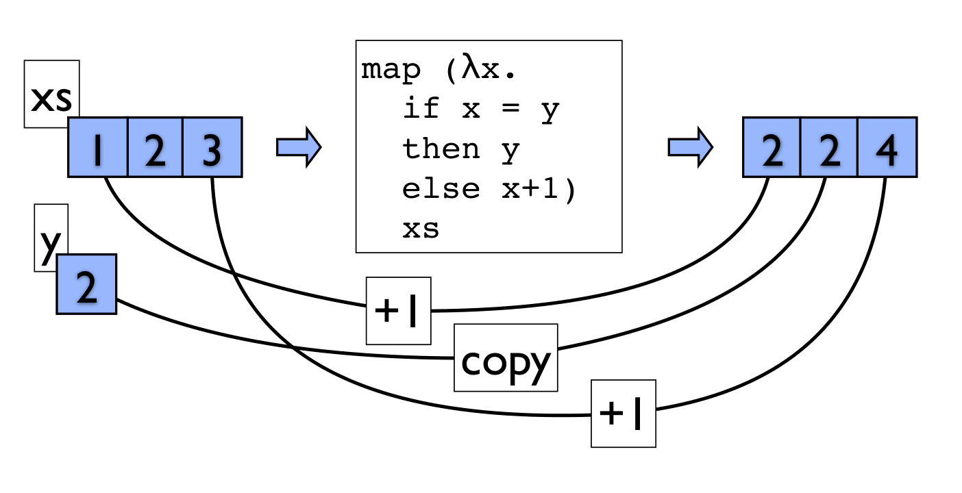
Figure 1 graphically illustrates these three forms of provenance on a single example: a simple function mapped over a list. This corresponds to the following TML sessions:

- val y = 2@L;
- fun f x = if x = y then y else x+1;
- val xs = [1@L1,2@L2,3@L3];
- val t = trace (map f xs);
val t = <trace> : ({L1:int,L2:int,L3:int}, int list) trace
- where t;
val it = [2@{},2@{L},4@{}]
- dependency t;
val it = [2@{L1,L},2@{L2,L},4@{L3,L}];
- expression t;
val it = [2@{L1+1},2@{L},4@{L3+1}];

Note that this illustrates much of the power of TML, including higher-order, recursive functions and sum, product and recursive types. We use this as a running example throughout the paper.

Refer to caption
Refer to caption
Refer to caption
Figure 1: Illustration of various forms of provenance

Provenance security.

The three models of provenance above represent useful forms of provenance that might increase users’ trust or confidence that they understand the results of a program. However, if the underlying data, or the structure of the computation, is sensitive, then making this information available may lead to inadvertent vulnerabilities, by making it possible for users to infer sensitive information that they cannot observe directly. This is a particular problem if we wish to disclose part of the result of a program, and provenance that justifies part of the result, while keeping other parts of the program’s execution, input, or output confidential.

As a simple example, consider a program 𝚒𝚏​x≠1​𝚝𝚑𝚎𝚗​(y,y)​𝚎𝚕𝚜𝚎​(z,w)\mathtt{if}~x\neq 1~\mathtt{then}~(y,y)~\mathtt{else}~(z,w). Suppose we wish to disclose some information about the computation to an untrusted recipient Alice (not necessarily a malicious attacker), that none of x,yx,y are visible to Alice, that z,wz,w are visible to Alice, and only the value of xx is confidential. If zz and ww happen to both equal a common value, say 4242, then the result is (42,42)(42,42). It is safe to disclose this result to Alice, because (without inspecting xx or yy) she cannot be certain whether x=1x=1, since there are two scenarios consistent with the result: x=1x=1 and y=42y=42 or x≠1x\neq 1 and yy arbitrary. However, any of the above forms of provenance make it possible to distinguish which branch was taken because the two different copies of 4242 in zz and ww will have different provenance. Thus, if the provenance information is released then a principal can infer that the second branch was taken, and hence, x=1x=1. In technical terms, we cannot disclose any of the above forms of provenance for the result while obfuscating the fact that x=1x=1.

To study these problems systematically, we introduce a single, general model of provenance that can be instantiated in different ways to obtain the other models mentioned above (among many others). Essentially, our approach is to record a detailed trace of evaluation, whose structure corresponds closely to that of a large-step operational semantics derivation. Other forms of provenance can then be extracted by traversing the trace, and the trace itself can be viewed as a form of provenance. Of course, naively recording such a detailed trace may be prohibitively expensive, and in this article we are not advocating that such traces be explicitly constructed in practical systems, only that they are useful as a formalism for understanding different forms of provenance and their security properties.

1.2 Summary

Contributions.

In this article, we build on, and refine, the provenance security framework previously introduced by Cheney [15]. We introduce a core language with replayable execution traces for a call-by-value, higher-order functional language, and make the following technical contributions:

  • •

    Refined definitions of obfuscation and disclosure (Sec. 2).

  • •

    A core calculus defining traced execution for a pure functional programming language (Sec. 3).

  • •

    A generic provenance extraction framework that includes several previously-studied forms of provenance as instances (Sec. 4).

  • •

    An analysis of disclosure and obfuscation guarantees provided by different forms of provenance, including techniques based on slicing execution traces (Sec. 5).

This article is a revised and expanded version of a conference paper [3]. Compared with the conference paper, this article includes detailed proofs, a more complete discussion of related work (including work published recently that was not covered in the conference paper), and additional examples and discussion of technical points. In addition, we encountered a problem with proving correctness of the disclosure slicing algorithm proposed in [3]; specifically, Lemma 2 in the conference version had a subtle problem, which we avoid through a reformulation of the disclosure slicing algorithm.

This article is also closely related to work on using traces for program slicing [40] published in ICFP 2012. The two papers present different aspects of a single research project; the trace model and some aspects of the slicing algorithms are closely related. However, the two papers make distinct contributions, and the system in the ICFP paper incorporates simplifications that are appropriate pragmatic choices for its application area (program slicing) but not appropriate for security analysis. Because of these differences we have chosen not to attempt to develop a unified presentation or implementation, to ensure that focus in this article remains on provenance security. We summarize the key differences below.

  • •

    In the ICFP paper, traces and slicing are defined in terms of an ad hoc semantics over partial values, and justified by a Galois connection between them. Here, we instead define slices for disclosure and obfuscation in terms of a standard operational semantics. One important consequence of these different choices is that unique minimal disclosure slices do not exist, whereas unique minimal backwards slices do exist in the ICFP paper.

  • •

    The slicing algorithms in the ICFP paper differ from those given here in certain technical details: specifically, we use value patterns and the ≂p\eqsim_{p} equivalence relation instead of partial values, and we use ◇{\Diamond}-patterns to support slicing of primitive operations instead of tagging primitive operations with the values of their inputs in traces.

  • •

    The ICFP paper did not present provenance extraction or explore the connection to provenance security that is the focus of this paper.

  • •

    The ICFP paper presents work on program slicing, differential slicing, and implementation techniques, topics that are beyond the scope of this article.

Outline.

Section 2 briefly recapitulates the framework introduced by Cheney [15] and refines some definitions. We present the (standard) syntax and tracing semantics of TML in Section 3. In Section 4 we introduce a framework for querying and extracting provenance views from traces, including the three models discussed above. Section 5 presents our main results about disclosure, obfuscation, and trace slicing. Section 6 presents related work and Section 7 concludes.

2 Background

We recapitulate the main components of the provenance security framework of Cheney [15]. The framework assumes a given set of abstract traces 𝒯\mathcal{T}, together with a collection 𝒬\mathcal{Q} of possible trace queries Q:𝒯→𝔹Q:\mathcal{T}\to\mathbb{B}, where 𝔹={0,1}\mathbb{B}=\{0,1\} is the set of Boolean truth values. These represent properties of traces that the system designer may want to protect or that legitimate users or attackers of the system may want to learn. In the previous paper, we considered refinements to take into account the knowledge of the principals about the possible system behaviors. In this article, we consider a single principal and assume that all traces 𝒯\mathcal{T} are considered possible, for simplicity.

Fix a set Ω\Omega of the possible provenance views, and a function P:𝒯→ΩP:\mathcal{T}\to\Omega mapping each trace to a provenance view of the trace. We may write (Ω,P:𝒯→Ω)(\Omega,P:\mathcal{T}\to\Omega) or just (Ω,P)(\Omega,P) for a provenance view. Also, we typically write q:Ω→𝔹q:\Omega\to\mathbb{B} for a provenance query, that is, a query on a provenance view.

Given this framework, we proposed the following definitions:

Definition 2.1  (Disclosure).

A query Q:𝒯→𝔹Q:\mathcal{T}\to\mathbb{B} is disclosed by a provenance view (Ω,P)(\Omega,P) if for every t,t′∈𝒯t,t^{\prime}\in\mathcal{T}, if P⁡(t)=P⁡(t′)P(t)=P(t^{\prime}) then Q⁡(t)=Q⁡(t′)Q(t)=Q(t^{\prime}).

In other words, disclosure means that there can be no traces t,t′t,t^{\prime} that have the same provenance view but where one satisfies the query and the other does not.

Definition 2.2  (Obfuscation).

A query Q:𝒯→𝔹Q:\mathcal{T}\to\mathbb{B} is obfuscated by a provenance view (Ω,P)(\Omega,P) if for every tt in 𝒯\mathcal{T}, there exists t′∈𝒯t^{\prime}\in\mathcal{T} such that P⁡(t)=P⁡(t′)P(t)=P(t^{\prime}) and Q⁡(t)≠Q⁡(t′)Q(t)\neq Q(t^{\prime}).

Thus, obfuscation is not exactly the opposite of disclosure; instead, it means that for every trace there is another trace with the same provenance view but different QQ-value. This means that a principal that has access to the provenance view but not the trace cannot be certain whether or not QQ is satisfied by the underlying trace.

In the previous paper, we gave several examples of instances of this framework. Here, for illustration, we just review one such instance, given by regular languages and finite automata.

Example 2.3  (Strings as traces).

Consider the regular sublanguage of {a,b}+\{a,b\}^{+} consisting of nonempty strings; these can be viewed as traces of an automaton or other sequential process. Some views of the traces of the automaton include a transducer T1T_{1} replacing each symbol with aa, a transducer T2T_{2} that deletes all of the aas, and a transducer T3T_{3} that deletes alternating symbols. A query over these traces can test whether the number of bbs is even; this is obfuscated by T1T_{1}, disclosed by T2T_{2}, and neither fully obfuscated nor fully disclosed by T3T_{3}.

When finite automata are used for queries and transducers for provenance views, we showed that disclosure is decidable for all queries and views and that obfuscation is decidable for all queries and views whose range is finite. It is unknown whether obfuscation is decidable in the general case.

The definitions above turn out to be too strong for our purposes; in this paper we will also consider some weaker versions of disclosure and obfuscation.

Definition 2.4.

A query Q:𝒯→𝔹Q:\mathcal{T}\to\mathbb{B} is positively disclosed by provenance view (Ω,P)(\Omega,P) via query q:Ω→𝔹q:\Omega\to\mathbb{B} if for every tt, if q⁡(P⁡(t))=1q(P(t))=1 then Q⁡(t)=1Q(t)=1.

A query Q:𝒯→𝔹Q:\mathcal{T}\to\mathbb{B} is negatively disclosed by provenance view (Ω,P)(\Omega,P) via query q:Ω→𝔹q:\Omega\to\mathbb{B} if for every tt, if q⁡(P⁡(t))=0q(P(t))=0 then Q⁡(t)=0Q(t)=0.

In other words, positive disclosure means that there is a query qq on the provenance that safely overapproximates QQ on the underlying trace. If q⁡(P⁡(t))q(P(t)) holds then we know Q⁡(t)Q(t) holds but otherwise we may not learn anything about tt. Dually, negative disclosure means that if q⁡(P⁡(t))q(P(t)) is false then we know Q⁡(t)Q(t) is also false, but otherwise learn nothing.

Example 2.5.

Suppose 𝒯=Ω={a,b}∗\mathcal{T}=\Omega=\{a,b\}^{*}. Define query Q⁡(t)Q(t) to be true if and only if tt is not of the form u⋅a​b​a​b⋅vu\cdot abab\cdot v for strings u,vu,v, and let P(a1a2⋯an)=a2a4⋯a⌊n2⌋P(a_{1}a_{2}\cdots a_{n})=a_{2}a_{4}\cdots a_{\lfloor\frac{n}{2}\rfloor}, the function that deletes alternate letters of its argument. Finally, let q⁡(t)q(t) be a query on Ω\Omega that is true if and only if tt has no substrings of the form a​aaa or b​bbb. Then QQ is positively disclosed by PP via qq, for if P⁡(t)P(t) has no a​aaa or b​bbb substring, then tt can have no a​b​a​babab substring. However, QQ is not negatively disclosed by PP (for any q′q^{\prime}), because, for example, P⁡(a​b​a​b)=b​b=P⁡(b​b​b​b)P(abab)=bb=P(bbbb).

Definition 2.6.

A query Q:𝒯→𝔹Q:\mathcal{T}\to\mathbb{B} is positively obfuscated by (Ω,P)(\Omega,P) if for every tt satisfying Q⁡(t)=1Q(t)=1 there exists a trace t′t^{\prime} such that Q⁡(t′)=0Q(t^{\prime})=0 and P⁡(t)=P⁡(t′)P(t)=P(t^{\prime}).

A query Q:𝒯→𝔹Q:\mathcal{T}\to\mathbb{B} is negatively obfuscated by (Ω,P)(\Omega,P) if for every tt satisfying Q⁡(t)=0Q(t)=0 there exists a trace t′t^{\prime} such that Q⁡(t′)=1Q(t^{\prime})=1 and P⁡(t)=P⁡(t′)P(t)=P(t^{\prime}).

In other words, positive obfuscation means that the provenance never reveals that QQ holds of the trace, but it may reveal that QQ fails. This weaker notion is useful for asserting that sensitive data is protected: if the sensitive data is not present in the trace then it is harmless to reveal this, but if the sensitive data is present then the provenance should hide enough information to make its presence uncertain. Dually, negative obfuscation means that the provenance view does not reveal ¬Q\neg Q.

Example 2.7.

Again suppose 𝒯=Ω={a,b}∗\mathcal{T}=\Omega=\{a,b\}^{*}. Define Q⁡(t)Q(t) to be true if and only if the number of aa symbols in tt is odd and false otherwise. Define P⁡(t)P(t) to be tt with all aas replaced by bbs. (In other words, P⁡(t)=b|t|P(t)=b^{|t|}, a string of bbs of the same length as tt.) PP positively obfuscates QQ because if Q⁡(t)Q(t) holds, then tt is a nonempty string with an odd number of aas, and we can form t′t^{\prime} such that P⁡(t)=P⁡(t′)P(t)=P(t^{\prime}) by replacing one of the aas of tt with a bb. However, PP does not negatively obfuscate QQ because P⁡(ϵ)=ϵP(\epsilon)=\epsilon and there is no other string t′t^{\prime} with Q⁡(t′)=t​r​u​eQ(t^{\prime})=true and P⁡(t′)=ϵP(t^{\prime})=\epsilon.

Proposition 2.8.

If PP both positively discloses and negatively discloses QQ via qq, then PP discloses QQ. Similarly, if PP both positively and negatively obfuscates QQ then PP obfuscates QQ.

Proof.

For the first part, suppose PP discloses QQ positively and negatively via qq. Let t,t′∈𝒯t,t^{\prime}\in\mathcal{T} be given where P⁡(t)=P⁡(t′)P(t)=P(t^{\prime}). If q⁡(P⁡(t))q(P(t)) holds then q⁡(P⁡(t′))q(P(t^{\prime})) holds so Q⁡(t)=1=Q⁡(t′)Q(t)=1=Q(t^{\prime}). If q⁡(P⁡(t))=0q(P(t))=0 then q⁡(P⁡(t′))=0q(P(t^{\prime}))=0 and so Q⁡(t)=0=Q⁡(t′)Q(t)=0=Q(t^{\prime}).

The argument for obfuscation is straightforward. ∎

Remark 2.9.

It may seem surprising that positive and negative disclosure specify a provenance query qq while full disclosure does not specify such a parameter. If full disclosure holds, then there is no need to mention the provenance query qq that answers trace queries over Ω\Omega, since it is the characteristic function of {P⁡(t)∣Q⁡(t)=1}\{P(t)\mid Q(t)=1\}. However, if we leave out (or existentially quantify over) the provenance query qq in positive or negative disclosure, then both definitions become trivial, since positive disclosure always holds for q⁡(x)=0q(x)=0 and negative disclosure always holds for q⁡(x)=1q(x)=1. Moreover, we want to be able to decompose proving full disclosure into proving positive and negative disclosure, but the argument given above requires that the positive and negative disclosure hold with respect to the same qq.

We now proceed to instantiate the framework with traces generated by a richer language, with corresponding notions of trace query and provenance view.

Typesτ:⁣:=b∣τ1×τ2∣τ1+τ2∣τ1→τ2∣μα.τ∣αType contextsΓ:⁣:=[x1:τ1,…,xn:τn]Code pointersκ:⁣:=f⁡(x).eMatchesm:⁣:={𝚒𝚗𝚕(x1).e1;𝚒𝚗𝚛(x2).e2}Valuesv:⁣:=c​∣(v1,v2)∣​𝚒𝚗𝚕​(v)​∣𝚒𝚗𝚛⁡(v)∣​⟨κ,γ⟩|𝚛𝚘𝚕𝚕⁡(v)Environmentsγ:⁣:=[x1↦v1,…,xn↦vn]Expressionse:⁣:=c|x​∣⊕(e¯)∣​𝚕𝚎𝚝​x=e1​𝚒𝚗​e2∣(e1,e2)​∣𝚏𝚜𝚝⁡(e)∣​𝚜𝚗𝚍​(e)∣𝚒𝚗𝚕⁡(e)​∣𝚒𝚗𝚛⁡(e)∣​𝚌𝚊𝚜𝚎​e​𝚘𝚏​m∣𝚏𝚞𝚗​κ|(e​e′)∣𝚛𝚘𝚕𝚕⁡(e)|𝚞𝚗𝚛𝚘𝚕𝚕⁡(e)TracesT:⁣:=c|x​∣⊕(T¯)∣​𝚕𝚎𝚝​x=T1​𝚒𝚗​T2∣(T1,T2)​∣𝚏𝚜𝚝⁡(T)∣​𝚜𝚗𝚍​(T)∣𝚒𝚗𝚕(T)∣𝚒𝚗𝚛(T)∣𝚌𝚊𝚜𝚎T⊳𝚒𝚗𝚕x.T1∣𝚌𝚊𝚜𝚎T⊳𝚒𝚗𝚛x.T2∣𝚏𝚞𝚗κ∣(T1T2)⊳κ,Γf(x).T∣𝚛𝚘𝚕𝚕⁡(T)|𝚞𝚗𝚛𝚘𝚕𝚕⁡(T)\begin{array}[]{@{}l@{\quad}r@{~~}c@{\quad}l}\mbox{Types}\hfil\hskip 9.24994pt&\tau&::=\hfil\hskip 9.24994pt&b\mid\tau_{1}\times\tau_{2}\mid\tau_{1}+\tau_{2}\mid\tau_{1}\rightarrow\tau_{2}\mid\mu{\alpha}.\tau\mid\alpha\\[2.84526pt] \mbox{Type contexts}\hfil\hskip 9.24994pt&\Gamma&::=\hfil\hskip 9.24994pt&[x_{1}:\tau_{1},\ldots,x_{n}:\tau_{n}]\\[2.84526pt] \mbox{Code pointers}\hfil\hskip 9.24994pt&\kappa&::=\hfil\hskip 9.24994pt&f(x).e\\[2.84526pt] \mbox{Matches}\hfil\hskip 9.24994pt&m&::=\hfil\hskip 9.24994pt&\{\mathtt{inl}(x_{1}).e_{1};\mathtt{inr}(x_{2}).e_{2}\}\\[2.84526pt] \mbox{Values}\hfil\hskip 9.24994pt&v&::=\hfil\hskip 9.24994pt&c\mid(v_{1},v_{2})\mid\mathtt{inl}(v)\mid\mathtt{inr}(v)\mid\langle\kappa,\gamma\rangle\mid\mathtt{roll}(v)\\[2.84526pt] \mbox{Environments}\hfil\hskip 9.24994pt&\gamma&::=\hfil\hskip 9.24994pt&[x_{1}\mapsto v_{1},\ldots,x_{n}\mapsto v_{n}]\\[2.84526pt] \mbox{Expressions}\hfil\hskip 9.24994pt&e&::=\hfil\hskip 9.24994pt&c\mid x\mid\oplus(\overline{e})\mid\mathtt{let}~{x=e_{1}}~\mathtt{in}~{e_{2}}\\[2.84526pt] \hfil\hskip 9.24994pt&&\mid\hfil\hskip 9.24994pt&(e_{1},e_{2})\mid\mathtt{fst}(e)\mid\mathtt{snd}(e)\\[2.84526pt] \hfil\hskip 9.24994pt&&\mid\hfil\hskip 9.24994pt&\mathtt{inl}(e)\mid\mathtt{inr}(e)\mid\mathtt{case}~e~\mathtt{of}~m\\[2.84526pt] \hfil\hskip 9.24994pt&&\mid\hfil\hskip 9.24994pt&\mathtt{fun}~\kappa\mid(e~e^{\prime})\\[2.84526pt] \hfil\hskip 9.24994pt&&\mid\hfil\hskip 9.24994pt&\mathtt{roll}(e)\mid\mathtt{unroll}(e)\\[5.69054pt] \mbox{Traces}\hfil\hskip 9.24994pt&T&::=\hfil\hskip 9.24994pt&c\mid x\mid\oplus(\overline{T})\mid\mathtt{let}~{x=T_{1}}~\mathtt{in}~{T_{2}}\\[2.84526pt] \hfil\hskip 9.24994pt&&\mid\hfil\hskip 9.24994pt&(T_{1},T_{2})\mid\mathtt{fst}(T)\mid\mathtt{snd}(T)\\[2.84526pt] \hfil\hskip 9.24994pt&&\mid\hfil\hskip 9.24994pt&\mathtt{inl}(T)\mid\mathtt{inr}(T)\mid\mathtt{case}~T\triangleright_{\mathtt{inl}}x.T_{1}\mid\mathtt{case}~T\triangleright_{\mathtt{inr}}x.T_{2}\\[2.84526pt] \hfil\hskip 9.24994pt&&\mid\hfil\hskip 9.24994pt&\mathtt{fun}~\kappa\mid(T_{1}~T_{2})\triangleright_{\kappa,\Gamma}f(x).T\\[2.84526pt] \hfil\hskip 9.24994pt&&\mid\hfil\hskip 9.24994pt&\mathtt{roll}(T)\mid\mathtt{unroll}(T)\end{array}
Figure 2: Abstract syntax of Core TML.

3 Core Language

We will develop a core language for provenance based on a standard, typed, call-by-value, pure language, called Transparent ML, or TML. For the purpose of this article, we focus on terminating runs of pure computations. We only consider terminating runs since otherwise there is no trace or end result to analyze; the question of how to deal with provenance in nonterminating or effectful programs is interesting, but left for future work. Allowing for effects or moving to a small-step semantics each seem likely to complicate the trace semantics (and subsequent analysis) considerably.

The syntax of TML types, expressions, and other syntactic classes is shown in Figure 2. The syntax of expressions and values is standard, following common textbook treatments of languages with binary pairs, binary sums, recursive types, and recursive functions [41]; constructs such as boolean conditionals, records, datatypes, or mutually recursive functions can be added without difficulty following the same pattern. We parameterize the syntax and semantics over primitive operations ⊕\oplus that take inputs of base type only; for example, equality on integers, arithmetic and boolean operations. In f⁡(x).ef(x).e, both ff and xx are variable names; ff is the name of the recursively defined function while xx is the name of the argument. Both ff and xx are bound in ee in an expression of the form f⁡(x).ef(x).e; generally, we adhere to the convention that in an expression of the form x.ex.e, variable xx is bound in ee.

We abbreviate functional terms of the form f⁡(x).ef(x).e using the letter κ\kappa, when convenient; similarly, we often abbreviate the expression {𝚒𝚗𝚕(x1).e1;𝚒𝚗𝚛(x2).e2}\{\mathtt{inl}(x_{1}).e_{1};\mathtt{inr}(x_{2}).e_{2}\} as mm. We sometimes refer to κ\kappa or mm as a code pointer or match pointer respectively; in a fixed program, there are a fixed finite number of such terms and so we can share them instead of explicitly copying them when used in traces.

The syntax of traces is also defined in Figure 2. Trace expressions TT have many syntactic forms in common with expressions; they differ primarily in the case and application trace forms, which include additional information showing how an application or case expression was evaluated. Traces can be viewed as witnessing terms for the operational derivation of an expression, and so their meaning is explained below along with that of the operational semantics rules. We will refer to trace expressions TT as TML-traces when necessary to distinguish them from abstract traces 𝒯\mathcal{T} introduced in the previous section.

3.1 Dynamic Semantics

γ,e⇓v,T\gamma,e\Downarrow v,T

γ,c⇓c,c​γ,x⇓γ⁡(x),x​γ,e¯⇓v¯,T¯γ,⊕(e¯)⇓⊕^​(v¯),⊕(T¯)​γ,e1⇓v1,T1γ[x↦v1],e2⇓v2,T2γ,𝚕𝚎𝚝​x=e1​𝚒𝚗​e2⇓v2,𝚕𝚎𝚝​x=T1​𝚒𝚗​T2​γ,e1⇓v1,T1​γ,e2⇓v2,T2γ,(e1,e2)⇓(v1,v2),(T1,T2)​γ,e⇓(v1,v2),Tγ,𝚏𝚜𝚝⁡(e)⇓v1,𝚏𝚜𝚝⁡(T)​γ,e⇓(v1,v2),Tγ,𝚜𝚗𝚍⁡(e)⇓v2,𝚜𝚗𝚍⁡(T)​γ,e⇓v,Tγ,𝚒𝚗𝚕⁡(e)⇓𝚒𝚗𝚕⁡(v),𝚒𝚗𝚕⁡(T)​(𝚒𝚗𝚕(x1).e1∈m)γ,e⇓𝚒𝚗𝚕(v),Tγ[x1↦v],e1⇓v1,T1γ,𝚌𝚊𝚜𝚎e𝚘𝚏m⇓v1,𝚌𝚊𝚜𝚎T⊳𝚒𝚗𝚕x1.T1​γ,e⇓v,Tγ,𝚒𝚗𝚛⁡(e)⇓𝚒𝚗𝚛⁡(v),𝚒𝚗𝚛⁡(T)​(𝚒𝚗𝚛(x2).e2∈m)γ,e⇓𝚒𝚗𝚛(v),Tγ[x2↦v],e2⇓v2,T2γ,𝚌𝚊𝚜𝚎e𝚘𝚏m⇓v2,𝚌𝚊𝚜𝚎T⊳𝚒𝚗𝚛x2.T2​γ,e⇓v,Tγ,𝚛𝚘𝚕𝚕⁡(e)⇓𝚛𝚘𝚕𝚕⁡(v),𝚛𝚘𝚕𝚕⁡(T)​γ,e⇓𝚛𝚘𝚕𝚕⁡(v),Tγ,𝚞𝚗𝚛𝚘𝚕𝚕⁡(e)⇓v,𝚞𝚗𝚛𝚘𝚕𝚕⁡(T)​γ,𝚏𝚞𝚗​κ⇓⟨κ,γ⟩,𝚏𝚞𝚗​κ​γ,e1⇓⟨κ,γ′⟩,T1(κ=f(x).e)γ,e2⇓v2,T2γ′[f↦⟨κ,γ′⟩,x↦v2],e⇓v,Tγ,(e1e2)⇓v,(T1T2)⊳κf(x).T\frac{}{\gamma,c\Downarrow c,c}\frac{}{\gamma,x\Downarrow\gamma(x),x}\frac{\gamma,\overline{e}\Downarrow\overline{v},\overline{T}}{\gamma,\oplus(\overline{e})\Downarrow\hat{\oplus}(\overline{v}),\oplus(\overline{T})}\frac{\gamma,e_{1}\Downarrow v_{1},T_{1}\hskip 9.24994pt\gamma[x\mapsto v_{1}],e_{2}\Downarrow v_{2},T_{2}}{\gamma,\mathtt{let}~{x=e_{1}}~\mathtt{in}~{e_{2}}\Downarrow v_{2},\mathtt{let}~{x=T_{1}}~\mathtt{in}~{T_{2}}}\\ \frac{\gamma,e_{1}\Downarrow v_{1},T_{1}\hskip 9.24994pt\gamma,e_{2}\Downarrow v_{2},T_{2}}{\gamma,(e_{1},e_{2})\Downarrow(v_{1},v_{2}),(T_{1},T_{2})}\frac{\gamma,e\Downarrow(v_{1},v_{2}),T}{\gamma,\mathtt{fst}(e)\Downarrow v_{1},\mathtt{fst}(T)}\frac{\gamma,e\Downarrow(v_{1},v_{2}),T}{\gamma,\mathtt{snd}(e)\Downarrow v_{2},\mathtt{snd}(T)}\\ \frac{\gamma,e\Downarrow v,T}{\gamma,\mathtt{inl}(e)\Downarrow\mathtt{inl}(v),\mathtt{inl}(T)}\frac{(\mathtt{inl}(x_{1}).e_{1}\in m)\hskip 9.24994pt\gamma,e\Downarrow\mathtt{inl}(v),T\hskip 9.24994pt\gamma[x_{1}\mapsto v],e_{1}\Downarrow v_{1},T_{1}}{\gamma,\mathtt{case}~e~\mathtt{of}~m\Downarrow v_{1},\mathtt{case}~T\triangleright_{\mathtt{inl}}x_{1}.T_{1}}\frac{\gamma,e\Downarrow v,T}{\gamma,\mathtt{inr}(e)\Downarrow\mathtt{inr}(v),\mathtt{inr}(T)}\frac{(\mathtt{inr}(x_{2}).e_{2}\in m)\hskip 9.24994pt\gamma,e\Downarrow\mathtt{inr}(v),T\hskip 9.24994pt\gamma[x_{2}\mapsto v],e_{2}\Downarrow v_{2},T_{2}}{\gamma,\mathtt{case}~e~\mathtt{of}~m\Downarrow v_{2},\mathtt{case}~T\triangleright_{\mathtt{inr}}x_{2}.T_{2}}\\ \frac{\gamma,e\Downarrow v,T}{\gamma,\mathtt{roll}(e)\Downarrow\mathtt{roll}(v),\mathtt{roll}(T)}\frac{\gamma,e\Downarrow\mathtt{roll}(v),T}{\gamma,\mathtt{unroll}(e)\Downarrow v,\mathtt{unroll}(T)}\\ \frac{}{\gamma,\mathtt{fun}~\kappa\Downarrow\langle\kappa,\gamma\rangle,\mathtt{fun}~\kappa}\frac{\gamma,e_{1}\Downarrow\langle\kappa,\gamma^{\prime}\rangle,T_{1}\hskip 9.24994pt(\kappa=f(x).e)\hskip 9.24994pt\gamma,e_{2}\Downarrow v_{2},T_{2}\hskip 9.24994pt\gamma^{\prime}[f\mapsto\langle\kappa,\gamma^{\prime}\rangle,x\mapsto v_{2}],e\Downarrow v,T}{\gamma,(e_{1}~e_{2})\Downarrow v,(T_{1}~T_{2})\triangleright_{\kappa}f(x).T}
Figure 3: Dynamic semantics of Core TML: rules for expression evaluation.

We augment a standard large-step operational semantics for TML by adding a parameter TT, which records a trace of the evaluation of the expression. The judgment γ,e⇓v,T\gamma,e\Downarrow v,T, defined in Figure 3, says that in environment γ\gamma, expression ee evaluates to value vv with trace TT.

If we ignore the trace parameter in this judgment, then the rules are essentially the standard ones for a call-by-value, pure functional language with pairs, sums, and recursive types and functions [41]. In particular, pairs are constructed by pairing and can be taken apart using the 𝚏𝚜𝚝\mathtt{fst} and 𝚜𝚗𝚍\mathtt{snd} operations. Values of sum type are constructed using the left and right injection operations 𝚒𝚗𝚕,𝚒𝚗𝚛\mathtt{inl},\mathtt{inr} and can be analyzed using the case expression, which examines a value of type τ1+τ2\tau_{1}+\tau_{2} and calls the appropriate branch with the injected value bound to a variable. Values of recursive type μ​α.τ\mu\alpha.\tau are constructed using 𝚛𝚘𝚕𝚕\mathtt{roll} and destructed using 𝚞𝚗𝚛𝚘𝚕𝚕\mathtt{unroll}; these operations indicate the explicit isomorphisms in the isorecursive treatment of recursive types. Finally, functions are (as usual) constructed using the function expression 𝚏𝚞𝚗​f​(x).e\mathtt{fun}~f(x).e and applied using function application e1​e2e_{1}~e_{2}.

Now if we consider the trace parameter, note that each rule has its own trace form, which builds the trace up from sub-traces obtained by the hypotheses of the rule. Traces can contain bound variables, reflecting the binding structure of the original expression. To illustrate, for let expressions, traces are similar to expressions:

𝚕𝚎𝚝​x=T1​𝚒𝚗​T2\mathtt{let}~{x=T_{1}}~\mathtt{in}~{T_{2}}

where we bind the variable in T2T_{2}.

The case and application evaluation traces record additional information about control flow. In either case, the first argument is evaluated to determine what expression to evaluate to obtain the final result. For case expressions, traces are of the form:

𝚌𝚊𝚜𝚎T⊳𝚒𝚗𝚕x1.T1𝚌𝚊𝚜𝚎T⊳𝚒𝚗𝚛x2.T2\mathtt{case}~T\triangleright_{\mathtt{inl}}x_{1}.T_{1}\quad\mathtt{case}~T\triangleright_{\mathtt{inr}}x_{2}.T_{2}

where we record the trace of the case scrutinee TT and the taken branch (T1T_{1} or T2T_{2}), and we re-bind the variable (x1x_{1} or x2x_{2}) in the trace of the taken branch. The subscript indicates which branch was taken. Similarly, for an application expression:

(T1T2)⊳κf(x).T(T_{1}~T_{2})\triangleright_{\kappa}f(x).T

we record the traces of the function subexpression T1T_{1}, the argument subexpression T2T_{2}, and the trace TT of the evaluation of the body of the function. The subscript κ=⟨f(x).e,Γ⟩\kappa=\langle f(x).e,\Gamma\rangle is a code pointer indicating the function and the typing environment of the call. The Γ\Gamma annotation is needed only to typecheck traces, so we usually elide it. Again, since the body trace can mention the function and argument names as free variables, we re-bind these variables.

We want to emphasize at this point that we do not necessarily expect that implementations routinely construct fully detailed traces along the above lines. Rather, the trace semantics is proposed here as a candidate for the most detailed form of provenance we will consider. Recording and compressing or filtering relevant information from traces in an efficient way is beyond the scope of this paper. However, some preliminary experiments in this direction have been performed in a recent paper on slicing for higher-order functional programs, based on a similar trace model [40].

Example 3.1.

Consider the factorial program expressed in Core TML:

let f = fun f(x). if x = 0 then 1 else x*(f(x-1))
in f 4

The trace of this program has the form

let f = fun f(x). e
in f 4    |> f(x).(e |>_else x * (
    f(x-1) |> f(x).(e |>_else x * (
     f(x-1) |> f(x).(e |>_else x * (
      f(x-1) |> f(x).(e |>_else x * (
       f(x-1) |> f(x).(e |>_then 1)))))))))

where e = if x = 0 then 1 else x*(f(x-1)). The trace reflects that ff calls itself four additional times when evaluating f​4f~4 and the 𝚎𝚕𝚜𝚎\mathtt{else}-branch is taken four times, and finally the 𝚝𝚑𝚎𝚗\mathtt{then}-branch is taken. Here, we use subscripts 𝚝𝚑𝚎𝚗\mathtt{then} and 𝚎𝚕𝚜𝚎\mathtt{else} to indicate the branch taken instead of 𝚒𝚗𝚕\mathtt{inl} and 𝚒𝚗𝚛\mathtt{inr}.

Remark 3.2.

The syntax of traces and expressions, and their corresponding evaluation rules, exhibit some redundancy. The syntax and semantics of expressions and traces could be fused so that both fall out as subsystems of one joint syntax / semantics. We adopt an explicit treatment for clarity, despite the resulting redundancy.

The operational semantics rules in Figures 3 and 4 illustrate a recipe that appears straightforward to follow in order to extend the system to a more realistic (pure) language; it is less clear how to extend the trace semantics to handle effects, nontermination, or other features. It may be interesting to try to capture the recipe as a formal construction over operational semantic specifications.

Trace Replay.

γ,T↷v\gamma,T\curvearrowright v

γ,c↷c​γ,x↷γ⁡(x)​γ,T¯↷v¯γ,⊕(T¯)↷⊕^​(v¯)​γ,T1↷v1γ[x↦v1],T2↷v2γ,𝚕𝚎𝚝​x=T1​𝚒𝚗​T2↷v2​γ,T1↷v1​γ,T2↷v2γ,(T1,T2)↷(v1,v2)​γ,T↷(v1,v2)γ,𝚏𝚜𝚝⁡(T)↷v1​γ,T↷(v1,v2)γ,𝚜𝚗𝚍⁡(T)↷v2​γ,T↷vγ,𝚒𝚗𝚕⁡(T)↷𝚒𝚗𝚕⁡(v)​γ,T↷𝚒𝚗𝚕(v)γ[x1↦v],T1↷v1γ,𝚌𝚊𝚜𝚎T⊳𝚒𝚗𝚕x1.T1↷v1​γ,T↷vγ,𝚒𝚗𝚛⁡(T)↷𝚒𝚗𝚛⁡(v)​γ,T↷𝚒𝚗𝚛(v)γ[x2↦v],T2↷v2γ,𝚌𝚊𝚜𝚎T⊳𝚒𝚗𝚛x2.T2↷v2​γ,T↷vγ,𝚛𝚘𝚕𝚕⁡(T)↷𝚛𝚘𝚕𝚕⁡(v)​γ,T↷𝚛𝚘𝚕𝚕⁡(v)γ,𝚞𝚗𝚛𝚘𝚕𝚕⁡(T)↷v​γ,𝚏𝚞𝚗​κ↷⟨κ,γ⟩​γ,T1↷⟨κ,γ′⟩γ,T2↷v2γ′[f↦⟨κ,γ′⟩,x↦v2],T↷vγ,(T1T2)⊳κf(x).T↷v\ \frac{}{\gamma,c\curvearrowright c}\frac{}{\gamma,x\curvearrowright\gamma(x)}\frac{\gamma,\overline{T}\curvearrowright\overline{v}}{\gamma,\oplus(\overline{T})\curvearrowright\hat{\oplus}(\overline{v})}\frac{\gamma,T_{1}\curvearrowright v_{1}\hskip 9.24994pt\gamma[x\mapsto v_{1}],T_{2}\curvearrowright v_{2}}{\gamma,\mathtt{let}~{x=T_{1}}~\mathtt{in}~{T_{2}}\curvearrowright v_{2}}\\ \frac{\gamma,T_{1}\curvearrowright v_{1}\hskip 9.24994pt\gamma,T_{2}\curvearrowright v_{2}\hskip 9.24994pt}{\gamma,(T_{1},T_{2})\curvearrowright(v_{1},v_{2})}\frac{\gamma,T\curvearrowright(v_{1},v_{2})}{\gamma,\mathtt{fst}(T)\curvearrowright v_{1}}\frac{\gamma,T\curvearrowright(v_{1},v_{2})}{\gamma,\mathtt{snd}(T)\curvearrowright v_{2}}\\ \frac{\gamma,T\curvearrowright v}{\gamma,\mathtt{inl}(T)\curvearrowright\mathtt{inl}(v)}\frac{\gamma,T\curvearrowright\mathtt{inl}(v)\hskip 9.24994pt\gamma[x_{1}\mapsto v],T_{1}\curvearrowright v_{1}}{\gamma,\mathtt{case}~T\triangleright_{\mathtt{inl}}x_{1}.T_{1}\curvearrowright v_{1}}\\ \frac{\gamma,T\curvearrowright v}{\gamma,\mathtt{inr}(T)\curvearrowright\mathtt{inr}(v)}\frac{\gamma,T\curvearrowright\mathtt{inr}(v)\hskip 9.24994pt\gamma[x_{2}\mapsto v],T_{2}\curvearrowright v_{2}}{\gamma,\mathtt{case}~T\triangleright_{\mathtt{inr}}x_{2}.T_{2}\curvearrowright v_{2}}\\ \frac{\gamma,T\curvearrowright v}{\gamma,\mathtt{roll}(T)\curvearrowright\mathtt{roll}(v)}\frac{\gamma,T\curvearrowright\mathtt{roll}(v)}{\gamma,\mathtt{unroll}(T)\curvearrowright{v}}\\ \frac{}{\gamma,\mathtt{fun}~\kappa\curvearrowright\langle\kappa,\gamma\rangle}\frac{\gamma,T_{1}\curvearrowright\langle\kappa,\gamma^{\prime}\rangle\hskip 9.24994pt\gamma,T_{2}\curvearrowright v_{2}\hskip 9.24994pt\gamma^{\prime}[f\mapsto\langle\kappa,\gamma^{\prime}\rangle,x\mapsto v_{2}],T\curvearrowright v}{\gamma,(T_{1}~T_{2})\triangleright_{\kappa}f(x).T\curvearrowright v}
Figure 4: Dynamic semantics of Core TML: rules for trace replay.

We equip traces with a semantics that relates them to expressions. We write γ,T↷v\gamma,T\curvearrowright v for the replay relation that reruns a trace on an environment (possibly different from the one originally used to construct TT). Figure 4 shows the rules for replaying traces. The rules for most trace forms are the same as the standard rules for evaluating the corresponding expression forms. Essentially, these rules require that the same control flow branches are taken as in the original run. If the input environment is different enough that the same branches cannot be taken, then replay fails.

Remark 3.3.

This behavior should be contrasted with traces used in self-adjusting computation [4, 2]. Such traces must always recompute the updated result; however, they typically operate at a coarser granularity by tracking reads and writes to memory locations. Moreover, the traces are essentially graphs built in memory using references and closures, so it is not straightforward to traverse such traces to obtain fine-grained information about what happened at run-time, as we shall do in Section 4.

Like evaluation, replay is deterministic, in that if a trace can be replayed on an environment then the resulting value is unique:

Theorem 3.4.

If γ,T↷v1\gamma,T\curvearrowright v_{1} and γ,T↷v2\gamma,T\curvearrowright v_{2} then v1=v2v_{1}=v_{2}.

Proof.

Proof is by (straightforward) structural induction on the first derivation and inversion on the second. ∎

3.2 Basic Properties of Traces

In this section, we identify key properties of traces, including type safety, and the consistency and fidelity properties that characterize how traces record the evaluation of an expression.

Determinacy and Type Safety.

We employ a standard type system for expressions. Figure 6 shows the (standard) typing rules for expressions and Figure 6 shows the rules for values and environments. Type checking requires a variable context Γ\Gamma that maps variables to types. We write Γ⊢e:τ\Gamma\vdash e:\tau to indicate that ee has type τ\tau in context Γ\Gamma. Similarly, we write Γ⊢𝚃T:τ\Gamma\vdash_{\mathtt{T}}T:\tau to indicate that TT is a well-formed trace of type τ\tau in context Γ\Gamma. Figure 7 shows the typing rules for traces. The unusual rules are those for case and application traces, whose form differs from the corresponding expression forms. One important point is that in the rule for application traces, the trace of the function body needs to typecheck in the same context Γ′\Gamma^{\prime} as the body of ee. This is why we allow the annotation Γ′\Gamma^{\prime} indicating the environment of the called function in application traces.

As noted above, expressions (and hence also traces) can be well-formed at more than one type, but this does not matter since we are not concerned with typechecking algorithms here.

Γ⊢e:τ\Gamma\vdash e:\tau

c:τ∈ΣΓ⊢c:τx:τ∈ΓΓ⊢x:τΓ⊢e¯:τ¯⊕:τ¯→τ′∈ΣΓ⊢⊕(e¯):τ′Γ⊢e1:τ1​Γ,x:τ1⊢e2:τ2Γ⊢𝚕𝚎𝚝​x=e1​𝚒𝚗​e2:τ2Γ⊢e1:τ1​Γ⊢e2:τ2Γ⊢(e1,e2):τ1×τ2Γ⊢e:τ1×τ2Γ⊢𝚏𝚜𝚝⁡(e):τ1Γ⊢e:τ1×τ2Γ⊢𝚜𝚗𝚍⁡(e):τ2Γ⊢e:τ1Γ⊢𝚒𝚗𝚕⁡(e):τ1+τ2Γ⊢e:τ2Γ⊢𝚒𝚗𝚛⁡(e):τ1+τ2Γ⊢e:τ1+τ2​Γ,x1:τ1⊢e1:τ​Γ,x2:τ2⊢e2:τΓ⊢𝚌𝚊𝚜𝚎x1𝚘𝚏{𝚒𝚗𝚕(e1).x2;𝚒𝚗𝚛(e2).e}:τΓ,f:τ1→τ2,x:τ1⊢e:τ2Γ⊢𝚏𝚞𝚗​f​(x).e:τ1→τ2Γ⊢e1:τ1→τ2​Γ⊢e2:τ1Γ⊢(e1​e2):τ2Γ⊢e:μ​α.τΓ⊢𝚞𝚗𝚛𝚘𝚕𝚕(e):τ[μα.τ/α]Γ⊢e:τ[μα.τ/α]Γ⊢𝚛𝚘𝚕𝚕⁡(e):μ​α.τ\frac{c:\tau\in\Sigma}{\Gamma\vdash c:\tau}\frac{x:\tau\in\Gamma}{\Gamma\vdash x:\tau}\frac{\Gamma\vdash\overline{e}:\overline{\tau}\hskip 9.24994pt\oplus:\overline{\tau}\to\tau^{\prime}\in\Sigma}{\Gamma\vdash\oplus(\overline{e}):\tau^{\prime}}\frac{\Gamma\vdash e_{1}:\tau_{1}\hskip 9.24994pt\Gamma,x:\tau_{1}\vdash e_{2}:\tau_{2}\hskip 9.24994pt}{\Gamma\vdash\mathtt{let}~{x=e_{1}}~\mathtt{in}~{e_{2}}:\tau_{2}}\\ \frac{\Gamma\vdash e_{1}:\tau_{1}\hskip 9.24994pt\Gamma\vdash e_{2}:\tau_{2}}{\Gamma\vdash(e_{1},e_{2}):\tau_{1}\times\tau_{2}}\frac{\Gamma\vdash e:\tau_{1}\times\tau_{2}}{\Gamma\vdash\mathtt{fst}(e):\tau_{1}}\frac{\Gamma\vdash e:\tau_{1}\times\tau_{2}}{\Gamma\vdash\mathtt{snd}(e):\tau_{2}}\\ \frac{\Gamma\vdash e:\tau_{1}}{\Gamma\vdash\mathtt{inl}(e):\tau_{1}+\tau_{2}}\frac{\Gamma\vdash e:\tau_{2}}{\Gamma\vdash\mathtt{inr}(e):\tau_{1}+\tau_{2}}\frac{\Gamma\vdash e:\tau_{1}+\tau_{2}\hskip 9.24994pt\Gamma,x_{1}:\tau_{1}\vdash e_{1}:\tau\hskip 9.24994pt\Gamma,x_{2}:\tau_{2}\vdash e_{2}:\tau}{\Gamma\vdash\mathtt{case}~x_{1}~\mathtt{of}~\{\mathtt{inl}(e_{1}).x_{2};\mathtt{inr}(e_{2}).e\}:\tau}\\ \frac{\Gamma,f:\tau_{1}\to\tau_{2},x:\tau_{1}\vdash e:\tau_{2}}{\Gamma\vdash\mathtt{fun}~f(x).e:\tau_{1}\to\tau_{2}}\frac{\Gamma\vdash e_{1}:\tau_{1}\to\tau_{2}\hskip 9.24994pt\Gamma\vdash e_{2}:\tau_{1}}{\Gamma\vdash(e_{1}~e_{2}):\tau_{2}}\\ \frac{\Gamma\vdash e:\mu{\alpha}.\tau}{\Gamma\vdash\mathtt{unroll}(e):\tau[\mu{\alpha}.\tau/\alpha]}\frac{\Gamma\vdash e:\tau[\mu{\alpha}.\tau/\alpha]}{\Gamma\vdash\mathtt{roll}(e):\mu{\alpha}.\tau}
Figure 5: Well-typed expressions of TML.

⊢v:τ\vdash v:\tau

c:τ∈Σ⊢c:τ⊢v1:τ1⊢v2:τ2⊢(v1,v2):τ1×τ2⊢v:τ1⊢𝚒𝚗𝚕⁡(v):τ1+τ2⊢v:τ2⊢𝚒𝚗𝚛⁡(v):τ1+τ2⊢γ:Γ​Γ,f:τ1→τ2,x:τ1⊢e:τ2⊢⟨⟨f(x).e,Γ⟩,γ⟩:τ1→τ2⊢v:τ[μα.τ/α]⊢𝚛𝚘𝚕𝚕⁡(v):μ​α.τ⊢v1:τ1⋯⊢vn:τn⊢[x1↦v1,…,xn↦vn]:[x1:τ1,…,xn:τn]\frac{c:\tau\in\Sigma}{\vdash c:\tau}\frac{\vdash v_{1}:\tau_{1}\hskip 9.24994pt\vdash v_{2}:\tau_{2}}{\vdash(v_{1},v_{2}):\tau_{1}\times\tau_{2}}\frac{\vdash v:\tau_{1}}{\vdash\mathtt{inl}(v):\tau_{1}+\tau_{2}}\frac{\vdash v:\tau_{2}}{\vdash\mathtt{inr}(v):\tau_{1}+\tau_{2}}\frac{\vdash\gamma:\Gamma\hskip 9.24994pt\Gamma,f:\tau_{1}\to\tau_{2},x:\tau_{1}\vdash e:\tau_{2}}{\vdash\langle\langle f(x).e,\Gamma\rangle,\gamma\rangle:\tau_{1}\to\tau_{2}}\frac{\vdash v:\tau[\mu{\alpha}.\tau/\alpha]}{\vdash\mathtt{roll}(v):\mu{\alpha}.\tau}\frac{\vdash v_{1}:\tau_{1}\hskip 9.24994pt\cdots\hskip 9.24994pt\vdash v_{n}:\tau_{n}}{\vdash[x_{1}\mapsto v_{1},\ldots,x_{n}\mapsto v_{n}]:[x_{1}:\tau_{1},\ldots,x_{n}:\tau_{n}]}
Figure 6: Value and environment typing.

Γ⊢𝚃T:τ\Gamma\vdash_{\mathtt{T}}T:\tau

c:τ∈ΣΓ⊢𝚃c:τx:τ∈ΓΓ⊢𝚃x:τΓ⊢𝚃T¯:τ¯⊕:τ¯→τ′∈ΣΓ⊢𝚃⊕(T¯):τ′Γ⊢𝚃T1:τ1Γ,x:τ1⊢𝚃T2:τ2Γ⊢𝚃𝚕𝚎𝚝x=T1𝚒𝚗T2:τ2Γ⊢𝚃T1:τ1Γ⊢𝚃T2:τ2Γ⊢𝚃(T1,T2):τ1×τ2Γ⊢𝚃T:τ1×τ2Γ⊢𝚃𝚏𝚜𝚝(T):τ1Γ⊢𝚃T:τ1×τ2Γ⊢𝚃𝚜𝚗𝚍(T):τ2Γ⊢𝚃T:τ1Γ⊢𝚃𝚒𝚗𝚕(T):τ1+τ2Γ⊢𝚃T:τ1+τ2Γ,x1:τ1⊢e1:τΓ,x2:τ2⊢e2:τΓ,x1:τ1⊢𝚃T1:τΓ⊢𝚃𝚌𝚊𝚜𝚎T𝚘𝚏{𝚒𝚗𝚕(x1).e1;𝚒𝚗𝚛(x2).e2}⊳𝚒𝚗𝚕x1.T1:τΓ⊢𝚃T:τ2Γ⊢𝚃𝚒𝚗𝚛(T):τ1+τ2Γ⊢𝚃T:τ1+τ2Γ,x1:τ1⊢e1:τΓ,x2:τ2⊢e2:τΓ,x2:τ2⊢𝚃T2:τΓ⊢𝚃𝚌𝚊𝚜𝚎T𝚘𝚏{𝚒𝚗𝚕(x1).e1;𝚒𝚗𝚛(x2).e2}⊳𝚒𝚗𝚛x2.T2:τΓ,f:τ1→τ2,x:τ1⊢e:τ2Γ⊢𝚃𝚏𝚞𝚗f(x).e:τ1→τ2Γ⊢𝚃T1:τ1→τ2Γ′,f:τ1→τ2,x:τ1⊢e:τ2Γ⊢𝚃T2:τ1Γ′,f:τ1→τ2,x:τ1⊢𝚃T:τ2Γ⊢𝚃(T1T2)⊳f⁡(x).e,Γ′f(x).T:τ2Γ⊢𝚃T:μα.τΓ⊢𝚃𝚞𝚗𝚛𝚘𝚕𝚕(T):τ[μα.τ/α]Γ⊢𝚃T:τ[μα.τ/α]Γ⊢𝚃𝚛𝚘𝚕𝚕(T):μα.τ\frac{c:\tau\in\Sigma}{\Gamma\vdash_{\mathtt{T}}c:\tau}\frac{x:\tau\in\Gamma}{\Gamma\vdash_{\mathtt{T}}x:\tau}\frac{\Gamma\vdash_{\mathtt{T}}\overline{T}:\overline{\tau}\hskip 9.24994pt\oplus:\overline{\tau}\to\tau^{\prime}\in\Sigma}{\Gamma\vdash_{\mathtt{T}}\oplus(\overline{T}):\tau^{\prime}}\frac{\Gamma\vdash_{\mathtt{T}}T_{1}:\tau_{1}\hskip 9.24994pt\Gamma,x:\tau_{1}\vdash_{\mathtt{T}}T_{2}:\tau_{2}\hskip 9.24994pt}{\Gamma\vdash_{\mathtt{T}}\mathtt{let}~{x=T_{1}}~\mathtt{in}~{T_{2}}:\tau_{2}}\\ \frac{\Gamma\vdash_{\mathtt{T}}T_{1}:\tau_{1}\hskip 9.24994pt\Gamma\vdash_{\mathtt{T}}T_{2}:\tau_{2}}{\Gamma\vdash_{\mathtt{T}}(T_{1},T_{2}):\tau_{1}\times\tau_{2}}\frac{\Gamma\vdash_{\mathtt{T}}T:\tau_{1}\times\tau_{2}}{\Gamma\vdash_{\mathtt{T}}\mathtt{fst}(T):\tau_{1}}\frac{\Gamma\vdash_{\mathtt{T}}T:\tau_{1}\times\tau_{2}}{\Gamma\vdash_{\mathtt{T}}\mathtt{snd}(T):\tau_{2}}\\ \frac{\Gamma\vdash_{\mathtt{T}}T:\tau_{1}}{\Gamma\vdash_{\mathtt{T}}\mathtt{inl}(T):\tau_{1}+\tau_{2}}\frac{\Gamma\vdash_{\mathtt{T}}T:\tau_{1}+\tau_{2}\hskip 9.24994pt\Gamma,x_{1}:\tau_{1}\vdash e_{1}:\tau\hskip 9.24994pt\Gamma,x_{2}:\tau_{2}\vdash e_{2}:\tau\hskip 9.24994pt\Gamma,x_{1}:\tau_{1}\vdash_{\mathtt{T}}T_{1}:\tau\hskip 9.24994pt}{\Gamma\vdash_{\mathtt{T}}\mathtt{case}~T~\mathtt{of}~\{\mathtt{inl}(x_{1}).e_{1};\mathtt{inr}(x_{2}).e_{2}\}\triangleright_{\mathtt{inl}}x_{1}.T_{1}:\tau}\\ \frac{\Gamma\vdash_{\mathtt{T}}T:\tau_{2}}{\Gamma\vdash_{\mathtt{T}}\mathtt{inr}(T):\tau_{1}+\tau_{2}}\frac{\Gamma\vdash_{\mathtt{T}}T:\tau_{1}+\tau_{2}\hskip 9.24994pt\Gamma,x_{1}:\tau_{1}\vdash e_{1}:\tau\hskip 9.24994pt\Gamma,x_{2}:\tau_{2}\vdash e_{2}:\tau\hskip 9.24994pt\Gamma,x_{2}:\tau_{2}\vdash_{\mathtt{T}}T_{2}:\tau\hskip 9.24994pt}{\Gamma\vdash_{\mathtt{T}}\mathtt{case}~T~\mathtt{of}~\{\mathtt{inl}(x_{1}).e_{1};\mathtt{inr}(x_{2}).e_{2}\}\triangleright_{\mathtt{inr}}x_{2}.T_{2}:\tau}\\ \frac{\Gamma,f:\tau_{1}\to\tau_{2},x:\tau_{1}\vdash e:\tau_{2}}{\Gamma\vdash_{\mathtt{T}}\mathtt{fun}~f(x).e:\tau_{1}\to\tau_{2}}\frac{\Gamma\vdash_{\mathtt{T}}T_{1}:\tau_{1}\to\tau_{2}\hskip 9.24994pt\Gamma^{\prime},f{:}\tau_{1}\to\tau_{2},x{:}\tau_{1}\vdash e:\tau_{2}\hskip 9.24994pt\Gamma\vdash_{\mathtt{T}}T_{2}:\tau_{1}\hskip 9.24994pt\Gamma^{\prime},f{:}\tau_{1}\to\tau_{2},x{:}\tau_{1}\vdash_{\mathtt{T}}T:\tau_{2}}{\Gamma\vdash_{\mathtt{T}}(T_{1}~T_{2})\triangleright_{f(x).e,\Gamma^{\prime}}f(x).T:\tau_{2}}\\ \frac{\Gamma\vdash_{\mathtt{T}}T:\mu{\alpha}.\tau}{\Gamma\vdash_{\mathtt{T}}\mathtt{unroll}(T):\tau[\mu{\alpha}.\tau/\alpha]}\frac{\Gamma\vdash_{\mathtt{T}}T:\tau[\mu{\alpha}.\tau/\alpha]}{\Gamma\vdash_{\mathtt{T}}\mathtt{roll}(T):\mu{\alpha}.\tau}
Figure 7: Well-typed traces of TML.
Theorem 3.5.

If Γ⊢e:τ\Gamma\vdash e:\tau and ⊢γ:Γ\vdash\gamma:\Gamma and γ,e⇓v,T\gamma,e\Downarrow v,T then ⊢v:τ\vdash v:\tau and Γ⊢𝚃T:τ\Gamma\vdash_{\mathtt{T}}T:\tau.

Proof.

Proof is by induction on the structure of the evaluation derivation, using inversion on the typing derivation. The only nonstandard cases are for the well-formedness of the trace, but these cases are straightforward. ∎

Replay is also type-safe in the obvious sense:

Theorem 3.6.

If Γ⊢𝚃T:τ\Gamma\vdash_{\mathtt{T}}T:\tau and ⊢γ:Γ\vdash\gamma:\Gamma and γ,T↷v\gamma,T\curvearrowright v then ⊢v:τ\vdash v:\tau.

Proof.

Proof is by induction on the structure of the replay derivation; most cases are similar to analogous cases for Theorem 3.5. ∎

Consistency and Fidelity.

We say that a trace TT is consistent with an environment γ\gamma if there exists vv such that γ,T↷v\gamma,T\curvearrowright v. A trace can easily be inconsistent with an environment, either because it is untyped nonsense and can never run (e.g. 𝚏𝚜𝚝⁡(42)\mathtt{fst}(42)), or, more interestingly, because replaying leads to situations that disagree with the control flow of the trace (e.g. while replaying 𝚌𝚊𝚜𝚎T⊳𝚒𝚗𝚕x1.T1\mathtt{case}~T\triangleright_{\mathtt{inl}}x_{1}.T_{1}, the replay of TT yields 𝚒𝚗𝚛⁡(v)\mathtt{inr}(v)).

Evaluation produces consistent traces, and replaying a trace on the same input yields the same value:

Theorem 3.7  (Consistency).

If γ,e⇓v,T\gamma,e\Downarrow v,T then γ,T↷v\gamma,T\curvearrowright v.

Proof.

Proof is by (straightforward) induction on the structure of derivations. ∎

The converse does not hold: a trace can be consistent without ever being produced by running a program. In particular, consistency does not check that the traces corresponding to bodies of function calls match the code pointers recorded in the trace. It is possible to refine the definition of replay so that the function bodies are checked against the traces, providing a stronger notion of consistency. However, this would complicate the replay semantics. In the rest of this article we usually consider traces obtained by running the tracing semantics. When this is the case, the derivation of γ,e⇓v,T\gamma,e\Downarrow v,T is itself a witness to this, so there is no need to introduce an additional judgment that captures this invariant.

Furthermore, the trace produced by evaluation is faithful to the original expression, in the sense that whenever the trace can be successfully replayed on a different input, the result (and its trace) is the same as what we would obtain by rerunning ee from scratch, and the resulting trace is the same as well. We call this property fidelity.

Theorem 3.8  (Fidelity).

If γ,e⇓v,T\gamma,e\Downarrow v,T and γ′,T↷v′\gamma^{\prime},T\curvearrowright v^{\prime} then γ′,e⇓v′,T\gamma^{\prime},e\Downarrow v^{\prime},T.

Proof.

Straightforward proof by induction on the structure of derivations. The interesting cases are for case and application expressions; in each case, the induction hypothesis ensures that the intermediate sum or function value encountered when recomputing ee in γ′\gamma^{\prime} matches that in the original derivation, so that the subtraces contingent on this value can be reused. ∎

Intuitively, fidelity corresponds to a repeatability or reproducibility property: it does not just guarantee that we get the same results when the trace is replayed on the same input, it also guarantees that the trace tells us what would happen if we rerun on inputs that are similar enough to the original input that replay can succeed. Thus, traces correspond to a form of explanation, analogous to forms of explanation explored in causal models and workflow provenance [14, 30, 31]. While we do not make more of this connection here, fidelity is also related to the correctness properties for various forms of slicing, including disclosure slicing (as discussed in Section 5).

Remark 3.9.

As noted at the beginning of the section, we made two simplifying assumptions: we consider traces only for terminating runs, and we exclude side-effects from the language. These assumptions are reasonable for many application areas of provenance (for example, in scientific computation and databases), but it is naturally of interest to consider extending our approaches to trace nonterminating or effectful computations. These raise potential complications: for example, adapting the trace semantics to a small-step semantics seems nontrivial, and it is not as clear what the appropriate correctness properties are for traces involving effects (including nondeterminism or allocation). These are interesting areas for exploration in future work.

4 Provenance Views and Extraction

In this section we consider different kinds of views and queries over provenance traces. To be specific, we consider a consistent triple (γ,T,v)(\gamma,T,v) where γ,T↷v\gamma,T\curvearrowright v to be the “traces” in the sense of the provenance security framework. Then queries over these triples correspond to sets of triples (generally definable using some compact syntax), and views correspond to functions from triples to some other data. We first consider a general class of views definable using annotation propagation, by giving a generic framework for extracting other kinds of provenance from execution traces. These forms of provenance induce provenance views in a natural way if we allow for initial annotations that uniquely identify each part of a value by a path.

4.1 Annotations, Paths, and Provenance Extraction

Many previous approaches to provenance can be viewed as performing a form of annotation propagation. The idea is to decorate the input with annotations (often, initially, unique identifiers) and propagate the annotations through the evaluation. For example, in where-provenance, annotations are optional tags that can be thought of as pointers showing where output data was copied from in the source [11, 10]. Other techniques, such as why-, how-, and dependency provenance, can also be defined in terms of annotation propagation [28, 27, 9, 18]. We gave similar definitions of different forms of provenance using a common framework for XQuery [13]; some of the properties proved are generalizations of properties shown there or in [10].

Based on this observation, we define a provenance extraction framework in which values are decorated with annotations and extraction functions take traces and return annotated values that can be interpreted as useful provenance information. We first define annotated values and give a generic annotation-propagation operation. We apply this framework to specify several concrete annotation schemes and extraction functions.

Annotations.

Let AA be an arbitrary set of annotations aa, which we usually assume includes a blank annotation ⊥\bot and a countably infinite set of identifiers ℓ∈Loc\ell\in\mathrm{Loc}, called locations. We define AA-annotated values v^\widehat{v} (or just annotated values, when AA is clear) using the following grammar:

v^\displaystyle\widehat{v} :⁣:=\displaystyle::= wa\displaystyle w^{a}
γ^\displaystyle\widehat{\gamma} :⁣:=\displaystyle::= [x1↦v^1,…,xn↦v^n]\displaystyle[x_{1}\mapsto\widehat{v}_{1},\ldots,x_{n}\mapsto\widehat{v}_{n}]
w\displaystyle w :⁣:=\displaystyle::= c​∣(v^1,v^2)∣​𝚒𝚗𝚕​(v^)​∣𝚒𝚗𝚛⁡(v^)∣​⟨κ,γ^⟩|𝚛𝚘𝚕𝚕⁡(v^)\displaystyle c\mid(\widehat{v}_{1},\widehat{v}_{2})\mid\mathtt{inl}(\widehat{v})\mid\mathtt{inr}(\widehat{v})\mid\langle\kappa,\widehat{\gamma}\rangle\mid\mathtt{roll}(\widehat{v})

We write γ^\widehat{\gamma} for annotated environments mapping variables to annotated values. We define an erasure function |v^||\widehat{v}| that maps each annotated value to an ordinary value by erasing the annotations. Similarly, |γ^||\widehat{\gamma}| is the ordinary environment obtained by erasing the annotations from the values of γ^\widehat{\gamma}. This function is defined mutually recursively on annotated values and environments as shown in Figure 9. We also introduce a notation for the set of annotated values occurring in a value in Figure 9. Moreover, we write

𝑜𝑐𝑐⊥̸(v^)={wa∈𝑜𝑐𝑐(v^)∣a≠⊥}\mathit{occ}^{\not\bot}(\widehat{v})=\{w^{a}\in\mathit{occ}(\widehat{v})\mid a\neq\bot\}

for the set of annotated values with annotation a≠⊥a\neq\bot.

|[x1↦v1,…,xn↦vn]|\displaystyle|[x_{1}\mapsto v_{1},\ldots,x_{n}\mapsto v_{n}]| =\displaystyle= [x1↦|v1|,…,xn↦|vn|]\displaystyle[x_{1}\mapsto|v_{1}|,\ldots,x_{n}\mapsto|v_{n}|]
|ca|\displaystyle|c^{a}| =\displaystyle= c\displaystyle c
|(v^1,v^2)a|\displaystyle|(\widehat{v}_{1},\widehat{v}_{2})^{a}| =\displaystyle= (|v^1|,|v^2|)\displaystyle(|\widehat{v}_{1}|,|\widehat{v}_{2}|)
|𝚒𝚗𝚕​(v^)a|\displaystyle|\mathtt{inl}(\widehat{v})^{a}| =\displaystyle= 𝚒𝚗𝚕⁡(|v^|)\displaystyle\mathtt{inl}(|\widehat{v}|)
|𝚒𝚗𝚛​(v^)a|\displaystyle|\mathtt{inr}(\widehat{v})^{a}| =\displaystyle= 𝚒𝚗𝚛⁡(|v^|)\displaystyle\mathtt{inr}(|\widehat{v}|)
|⟨κ,γ^⟩a|\displaystyle|\langle\kappa,\widehat{\gamma}\rangle^{a}| =\displaystyle= ⟨κ,|γ^|⟩\displaystyle\langle\kappa,|\widehat{\gamma}|\rangle
|𝚛𝚘𝚕𝚕​(v^)a|\displaystyle|\mathtt{roll}(\widehat{v})^{a}| =\displaystyle= 𝚛𝚘𝚕𝚕⁡(|v^|)\displaystyle\mathtt{roll}(|\widehat{v}|)
Figure 8: Erasure operation.
𝑜𝑐𝑐⁡(ca)\displaystyle\mathit{occ}(c^{a}) =\displaystyle= {ca}\displaystyle\{c^{a}\}
𝑜𝑐𝑐⁡((v^1,v^2)a)\displaystyle\mathit{occ}((\widehat{v}_{1},\widehat{v}_{2})^{a}) =\displaystyle= {(v^1,v^2)a}∪𝑜𝑐𝑐⁡(v^1)∪𝑜𝑐𝑐⁡(v^2)\displaystyle\{(\widehat{v}_{1},\widehat{v}_{2})^{a}\}\cup\mathit{occ}(\widehat{v}_{1})\cup\mathit{occ}(\widehat{v}_{2})
𝑜𝑐𝑐⁡((𝚒𝚗𝚕⁡(v^))a)\displaystyle\mathit{occ}((\mathtt{inl}(\widehat{v}))^{a}) =\displaystyle= {(𝚒𝚗𝚕⁡(v^))a}∪𝑜𝑐𝑐⁡(v^)\displaystyle\{(\mathtt{inl}(\widehat{v}))^{a}\}\cup\mathit{occ}(\widehat{v})
𝑜𝑐𝑐⁡((𝚒𝚗𝚛⁡(v^))a)\displaystyle\mathit{occ}((\mathtt{inr}(\widehat{v}))^{a}) =\displaystyle= {(𝚒𝚗𝚛⁡(v^))a}∪𝑜𝑐𝑐⁡(v^)\displaystyle\{(\mathtt{inr}(\widehat{v}))^{a}\}\cup\mathit{occ}(\widehat{v})
𝑜𝑐𝑐⁡((𝚛𝚘𝚕𝚕⁡(v^))a)\displaystyle\mathit{occ}((\mathtt{roll}(\widehat{v}))^{a}) =\displaystyle= {(𝚛𝚘𝚕𝚕⁡(v^))a}∪𝑜𝑐𝑐⁡(v^)\displaystyle\{(\mathtt{roll}(\widehat{v}))^{a}\}\cup\mathit{occ}(\widehat{v})
𝑜𝑐𝑐⁡(⟨κ,γ^⟩a)\displaystyle\mathit{occ}(\langle\kappa,\widehat{\gamma}\rangle^{a}) =\displaystyle= {⟨κ,γ^⟩a}∪𝑜𝑐𝑐⁡(γ^)\displaystyle\{\langle\kappa,\widehat{\gamma}\rangle^{a}\}\cup\mathit{occ}(\widehat{\gamma})
𝑜𝑐𝑐⁡(γ^)\displaystyle\mathit{occ}(\widehat{\gamma}) =\displaystyle= ⋃x∈dom⁡(γ^)𝑜𝑐𝑐​(γ^​(x))\displaystyle\bigcup_{x\in\mathrm{dom}(\widehat{\gamma})}\mathit{occ}(\widehat{\gamma}(x))
Figure 9: Occurrences of annotated values.

Paths as annotations.

For annotations to be useful when the full input is unavailable, we consider annotations where the locations ℓ\ell are paths that uniquely address parts of the input environment. Paths π\pi have syntax:

π::=ϵ∣x.π∣1.π∣2.π\pi::=\epsilon\mid x.\pi\mid 1.\pi\mid 2.\pi

and we consider path concatenation π.π′\pi.\pi^{\prime} to be associative with unit ϵ\epsilon, so that we may write π.i\pi.i to construct a pattern ending in ii. Paths address parts of values or environments; we write v⁡[π]v[\pi] or γ⁡[π]\gamma[\pi] for the part of vv or γ\gamma addressed by π\pi, defined in Figure 10.

v⁡[ϵ]\displaystyle v[\epsilon] =\displaystyle= v\displaystyle v
(v1,v2)[1.π]\displaystyle(v_{1},v_{2})[1.\pi] =\displaystyle= v1​[π]\displaystyle v_{1}[\pi]
(v1,v2)[2.π]\displaystyle(v_{1},v_{2})[2.\pi] =\displaystyle= v2​[π]\displaystyle v_{2}[\pi]
(𝚒𝚗𝚕(v))[1.π]\displaystyle(\mathtt{inl}(v))[1.\pi] =\displaystyle= v⁡[π]\displaystyle v[\pi]
(𝚒𝚗𝚛(v))[1.π]\displaystyle(\mathtt{inr}(v))[1.\pi] =\displaystyle= v⁡[π]\displaystyle v[\pi]
(𝚛𝚘𝚕𝚕(v))[1.π]\displaystyle(\mathtt{roll}(v))[1.\pi] =\displaystyle= v⁡[π]\displaystyle v[\pi]
(⟨κ,γ⟩)[1.π]\displaystyle(\langle\kappa,\gamma\rangle)[1.\pi] =\displaystyle= γ⁡[π]\displaystyle\gamma[\pi]
γ[x.π]\displaystyle\gamma[x.\pi] =\displaystyle= γ​(x)​[π]\displaystyle\gamma(x)[\pi]
Figure 10: Path lookup operation.

We write 𝗉𝖺𝗍𝗁⁡(γ)\mathsf{path}(\gamma) for the environment γ\gamma with each component annotated with the path to that component. More generally, we define 𝗉𝖺𝗍𝗁π​(γCLOSE\mathsf{path}_{\pi}(\gamma) and 𝗉𝖺𝗍𝗁π​(v)\mathsf{path}_{\pi}(v) as shown in Figure 11. Then 𝗉𝖺𝗍𝗁​(v)=𝗉𝖺𝗍𝗁ϵ​(v)\mathsf{path}(v)=\mathsf{path}_{\epsilon}(v) and 𝗉𝖺𝗍𝗁⁡(γ)=𝗉𝖺𝗍𝗁ϵ​(γ)\mathsf{path}(\gamma)=\mathsf{path}_{\epsilon}(\gamma). For example, 𝗉𝖺𝗍𝗁([x↦(1,2),y↦𝚒𝚗𝚕(4)])=[x↦(1x​.1,2x​.2)x,y↦𝚒𝚗𝚕(4y​.1)y]\mathsf{path}([x\mapsto(1,2),y\mapsto\mathtt{inl}(4)])=[x\mapsto(1^{x.1},2^{x.2})^{x},y\mapsto\mathtt{inl}(4^{y.1})^{y}].

𝗉𝖺𝗍𝗁π​(γ)\displaystyle\mathsf{path}_{\pi}(\gamma) =\displaystyle= [x1↦𝗉𝖺𝗍𝗁π.x1(γ(x1)),…,xn↦𝗉𝖺𝗍𝗁π.xn(γ(xn))]\displaystyle[x_{1}\mapsto\mathsf{path}_{\pi.x_{1}}(\gamma(x_{1})),\ldots,x_{n}\mapsto\mathsf{path}_{\pi.x_{n}}(\gamma(x_{n}))]
𝗉𝖺𝗍𝗁π​(c)\displaystyle\mathsf{path}_{\pi}(c) =\displaystyle= cπ\displaystyle c^{\pi}
𝗉𝖺𝗍𝗁π​((v1,v2))\displaystyle\mathsf{path}_{\pi}((v_{1},v_{2})) =\displaystyle= (𝗉𝖺𝗍𝗁π​.1​(v1),𝗉𝖺𝗍𝗁π​.2​(v2))π\displaystyle(\mathsf{path}_{\pi.1}(v_{1}),\mathsf{path}_{\pi.2}(v_{2}))^{\pi}
𝗉𝖺𝗍𝗁π​(𝚒𝚗𝚕​(v))\displaystyle\mathsf{path}_{\pi}(\mathtt{inl}(v)) =\displaystyle= 𝚒𝚗𝚕​(𝗉𝖺𝗍𝗁π​.1​(v))π\displaystyle\mathtt{inl}(\mathsf{path}_{\pi.1}(v))^{\pi}
𝗉𝖺𝗍𝗁π​(𝚒𝚗𝚛​(v))\displaystyle\mathsf{path}_{\pi}(\mathtt{inr}(v)) =\displaystyle= 𝚒𝚗𝚛​(𝗉𝖺𝗍𝗁π​.1​(v))π\displaystyle\mathtt{inr}(\mathsf{path}_{\pi.1}(v))^{\pi}
𝗉𝖺𝗍𝗁π​(⟨κ,γ⟩)\displaystyle\mathsf{path}_{\pi}(\langle\kappa,\gamma\rangle) =\displaystyle= ⟨κ,𝗉𝖺𝗍𝗁π​.1​(γ)⟩π\displaystyle\langle\kappa,\mathsf{path}_{\pi.1}(\gamma)\rangle^{\pi}
Figure 11: Path annotation operation.

Extraction framework.

We will define a family of provenance extraction functions 𝖥⁡(T,γ^)\mathsf{F}(T,\widehat{\gamma}) that take a trace TT and an environment γ^\widehat{\gamma} and return an annotated value. Each such 𝖥\mathsf{F} can be specified by giving the following annotation-propagation functions:

𝖥c,𝖥κ\displaystyle\mathsf{F}_{c},\mathsf{F}_{\kappa} :\displaystyle: A\displaystyle A
𝖥1,𝖥2,𝖥L,𝖥R,𝖥𝚊𝚙𝚙,𝖥𝚞𝚗𝚛𝚘𝚕𝚕\displaystyle\mathsf{F}_{1},\mathsf{F}_{2},\mathsf{F}_{L},\mathsf{F}_{R},\mathsf{F}_{\mathtt{app}},\mathsf{F}_{\mathtt{unroll}} :\displaystyle: A×A→A\displaystyle A\times A\to A
𝖥⊕\displaystyle\mathsf{F}_{\oplus} :\displaystyle: An→A(where ⊕ is n-ary)\displaystyle A^{n}\to A\qquad(\text{where $\oplus$ is $n$-ary})

Each function shows how the annotations involved in the corresponding computational step propagate to the result. For example, 𝖥1​(a,b)\mathsf{F}_{1}(a,b) gives the annotation on the result of a 𝚏𝚜𝚝\mathtt{fst}-projection, where aa is the annotation on the pair and bb is the annotation of the first element. Figure 12 shows how to propagate annotations through a trace given basic annotation-propagation functions.

𝖥⁡(x,γ^)=γ^​(x)𝖥⁡(𝚕𝚎𝚝​x=T1​𝚒𝚗​T2,γ^)=𝖥(T2,γ^[x↦𝖥(T1,γ^)])𝖥⁡(c,γ^)=c𝖥c𝖥⁡(⊕(T1,…,Tn),γ^)=(⊕^​(c1,…,cn))𝖥⊕​(a1,…,an)whereciai=𝖥⁡(Ti,γ^)𝖥⁡((T1,T2),γ^)=(𝖥⁡(T1,γ^),𝖥⁡(T2,γ^))⊥𝖥⁡(𝚏𝚜𝚝⁡(T),γ^)=v1𝖥1​(a,b)where(v1b,v^2)a=𝖥⁡(T,γ^)𝖥⁡(𝚜𝚗𝚍⁡(T),γ^)=v2𝖥2​(a,b)where(v^1,v2b)a=𝖥⁡(T,γ^)𝖥⁡(𝚒𝚗𝚕⁡(T),γ^)=𝚒𝚗𝚕​(𝖥⁡(T,γ^))⊥𝖥⁡(𝚒𝚗𝚛⁡(T),γ^)=𝚒𝚗𝚛​(𝖥⁡(T,γ^))⊥𝖥((𝚌𝚊𝚜𝚎T)⊳𝚒𝚗𝚕x.T1,γ^)=v𝖥L​(a,b)where𝚒𝚗𝚕​(v^)a=𝖥⁡(T,γ^)andvb=𝖥(T1,γ^[y↦v^])𝖥((𝚌𝚊𝚜𝚎T)⊳𝚒𝚗𝚛y.T2,γ^)=v𝖥R​(a,b)where𝚒𝚗𝚛​(v^)a=𝖥⁡(T,γ^)andvb=𝖥(T2,γ^[y↦v^])𝖥⁡(𝚏𝚞𝚗​κ,γ^)=⟨κ,γ^⟩𝖥κ𝖥((T1T2)⊳κf(x).T,γ^)=v𝖥𝚊𝚙𝚙​(a,b)where⟨κ,γ^′⟩a=𝖥⁡(T1,γ^)andv^2=𝖥⁡(T2,γ^)andvb=𝖥(T,γ^′[f↦⟨κ,γ^′⟩a,x↦v^2]))𝖥⁡(𝚛𝚘𝚕𝚕⁡(T),γ^)=𝚛𝚘𝚕𝚕​(𝖥⁡(T,γ^))⊥𝖥⁡(𝚞𝚗𝚛𝚘𝚕𝚕⁡(T),γ^)=v𝖥𝚞𝚗𝚛𝚘𝚕𝚕​(a,b)where𝚛𝚘𝚕𝚕​(vb)a=𝖥⁡(T,γ^)\small\begin{array}[]{rclll}\mathsf{F}(x,\widehat{\gamma})&=&\widehat{\gamma}(x)\\[1.0pt] \mathsf{F}(\mathtt{let}~{x=T_{1}}~\mathtt{in}~{T_{2}},\widehat{\gamma})&=&\mathsf{F}(T_{2},\widehat{\gamma}[x{\mapsto}\mathsf{F}(T_{1},\widehat{\gamma})])\\[1.0pt] \mathsf{F}(c,\widehat{\gamma})&=&c^{\mathsf{F}_{c}}\\[1.0pt] \mathsf{F}(\oplus(T_{1},\ldots,T_{n}),\widehat{\gamma})&=&(\hat{\oplus}(c_{1},\ldots,c_{n}))^{\mathsf{F}_{\oplus}(a_{1},\ldots,a_{n})}&\text{where}&c_{i}^{a_{i}}=\mathsf{F}(T_{i},\widehat{\gamma})\\[1.0pt] \mathsf{F}((T_{1},T_{2}),\widehat{\gamma})&=&(\mathsf{F}(T_{1},\widehat{\gamma}),\mathsf{F}(T_{2},\widehat{\gamma}))^{\bot}\\[1.0pt] \mathsf{F}(\mathtt{fst}(T),\widehat{\gamma})&=&v_{1}^{\mathsf{F}_{1}(a,b)}&\text{where}&(v_{1}^{b},\widehat{v}_{2})^{a}=\mathsf{F}(T,\widehat{\gamma})\\[1.0pt] \mathsf{F}(\mathtt{snd}(T),\widehat{\gamma})&=&v_{2}^{\mathsf{F}_{2}(a,b)}&\text{where}&(\widehat{v}_{1},v_{2}^{b})^{a}=\mathsf{F}(T,\widehat{\gamma})\\[1.0pt] \mathsf{F}(\mathtt{inl}(T),\widehat{\gamma})&=&\mathtt{inl}(\mathsf{F}(T,\widehat{\gamma}))^{\bot}\\[1.0pt] \mathsf{F}(\mathtt{inr}(T),\widehat{\gamma})&=&\mathtt{inr}(\mathsf{F}(T,\widehat{\gamma}))^{\bot}\\[1.0pt] \mathsf{F}((\mathtt{case}~T)\triangleright_{\mathtt{inl}}x.T_{1},\widehat{\gamma})&=&v^{\mathsf{F}_{L}(a,b)}&\text{where}&\mathtt{inl}(\widehat{v})^{a}=\mathsf{F}(T,\widehat{\gamma})\\ &&&\text{and}&v^{b}=\mathsf{F}(T_{1},\widehat{\gamma}[y{\mapsto}\widehat{v}])\\[1.0pt] \mathsf{F}((\mathtt{case}~T)\triangleright_{\mathtt{inr}}y.T_{2},\widehat{\gamma})&=&v^{\mathsf{F}_{R}(a,b)}&\text{where}&\mathtt{inr}(\widehat{v})^{a}=\mathsf{F}(T,\widehat{\gamma})\\ &&&\text{and}&v^{b}=\mathsf{F}(T_{2},\widehat{\gamma}[y{\mapsto}\widehat{v}])\\[1.0pt] \mathsf{F}(\mathtt{fun}~\kappa,\widehat{\gamma})&=&\langle\kappa,\widehat{\gamma}\rangle^{\mathsf{F}_{\kappa}}\\[1.0pt] \mathsf{F}((T_{1}~T_{2})\triangleright_{\kappa}f(x).T,\widehat{\gamma})&=&v^{\mathsf{F}_{\mathtt{app}}(a,b)}&\text{where}&\langle\kappa,\widehat{\gamma}^{\prime}\rangle^{a}=\mathsf{F}(T_{1},\widehat{\gamma})\\ &&&\text{and}&\widehat{v}_{2}=\mathsf{F}(T_{2},\widehat{\gamma})\\ &&&\text{and}&v^{b}=\mathsf{F}(T,\widehat{\gamma}^{\prime}[f{\mapsto}\langle\kappa,\widehat{\gamma}^{\prime}\rangle^{a},x{\mapsto}\widehat{v}_{2}]))\\[1.0pt] \mathsf{F}(\mathtt{roll}(T),\widehat{\gamma})&=&\mathtt{roll}(\mathsf{F}(T,\widehat{\gamma}))^{\bot}\\[1.0pt] \mathsf{F}(\mathtt{unroll}(T),\widehat{\gamma})&=&v^{\mathsf{F}_{\mathtt{unroll}}(a,b)}&\text{where}&\mathtt{roll}(v^{b})^{a}=\mathsf{F}(T,\widehat{\gamma})\end{array}
Figure 12: Generic extraction.
Remark 4.1.

The extraction framework hard-wires the behavior of certain operations such as 𝚕𝚎𝚝\mathtt{let}, 𝚒𝚗𝚕⁡()\mathtt{inl}(), 𝚒𝚗𝚛⁡()\mathtt{inr}(),𝚛𝚘𝚕𝚕⁡()\mathtt{roll}(), and pairing, using ⊥\bot to handle all of them. On the other hand, even though these constructors are hard-wired so that the top-level annotation is always ⊥\bot, this does not imply that the first arguments supplied to the corresponding extraction functions 𝖥1,𝖥2\mathsf{F}_{1},\mathsf{F}_{2}, etc. are always ⊥\bot; see Example 4.13 for an illustration of this point.

It would also be possible to extend the framework to allow greater customization; however, this functionality is not needed by any of the forms of provenance in this article. We believe that the framework presented in this paper is general enough to be of use beyond the three provenance models we considered, but we do not know how one could prove that it is general enough for all purposes — or how one could prove that any alternative framework is general enough for all purposes. It is also possible that there are natural forms of provenance that do not fit (a reasonable generalization of) the framework.

Theorem 4.2.

Every generic provenance extraction function is compatible with replay: that is, for any γ^,T,v\widehat{\gamma},T,v, if |γ^|,T↷v|\widehat{\gamma}|,T\curvearrowright v then |𝖥⁡(T,γ^)|=v|\mathsf{F}(T,\widehat{\gamma})|=v.

Proof.

Straightforward induction on replay derivations. ∎

Remark 4.3.

Consider the trivial annotation structure 𝖳𝗋𝗂𝗏\mathsf{Triv} with underlying annotation set {⊥}\{\bot\}. In this setting, the erasure function |−||-| is bijective; its inverse just decorates each part of a value with ⊥\bot. Consider also a trivial instance of the generic provenance framework for {⊥}\{\bot\} such that 𝖳𝗋𝗂𝗏κ=⊥\mathsf{Triv}_{\kappa}=\bot and 𝖳𝗋𝗂𝗏c=⊥\mathsf{Triv}_{c}=\bot and all of the annotation-propagation functions are constant functions returning ⊥\bot, that is, 𝖳𝗋𝗂𝗏1(x,y)=⊥\mathsf{Triv}_{1}(x,y)=\bot, etc. This instance of the provenance framework is essentially the same as the trace replay semantics defined by the judgment γ,T↷v\gamma,T\curvearrowright v. Thus, the generic extraction framework can be viewed as a denotational presentation of the replay semantics of traces, generalized to allow for annotated values.

Where-provenance.

Where-provenance can be defined via an annotation-propagating semantics where annotations are either labels ℓ\ell or the blank annotation ⊥\bot. Intuitively, for where-provenance, an explicit label ℓ\ell annotating a part of the input indicates that that part “comes from” a part of the input with the same label; an annotation ⊥\bot provides no information about where the output part “comes from” in the input (if anywhere). We define the where-provenance semantics 𝖶⁡(T,γ^)\mathsf{W}(T,\widehat{\gamma}) using the following annotation-propagation functions:

𝖶c,𝖶κ\displaystyle\mathsf{W}_{c},\mathsf{W}_{\kappa} =\displaystyle= ⊥\displaystyle\bot
𝖶1,𝖶2,𝖶L,𝖶R,𝖶𝚊𝚙𝚙,𝖶𝚞𝚗𝚛𝚘𝚕𝚕\displaystyle\mathsf{W}_{1},\mathsf{W}_{2},\mathsf{W}_{L},\mathsf{W}_{R},\mathsf{W}_{\mathtt{app}},\mathsf{W}_{\mathtt{unroll}} =\displaystyle= λ⁡(x,y).y\displaystyle\lambda(x,y).y
𝖶⊕\displaystyle\mathsf{W}_{\oplus} =\displaystyle= λ⁡(a1,…,an).⊥\displaystyle\lambda(a_{1},\ldots,a_{n}).\bot

Essentially, these functions preserve the annotations of data that are copied, and annotate computed or constructed data with ⊥\bot. This semantics is similar to that in Buneman et al. [10] and previous treatments of where-provenance in databases, adapted to TML. Figure 13 shows the generic semantics specialized to where-provenance. Note that for a function like “factorial”, the where-provenance of the output is always ⊥\bot.

𝖶⁡(c,γ^)=c⊥𝖶⁡(⊕(T1,…,Tn),γ^)=(⊕^​(c1,…,cn))⊥whereciai=𝖶⁡(Ti,γ^)𝖶⁡(𝚏𝚜𝚝⁡(T),γ^)=v^1where(v^1,v^2)a=𝖶⁡(T,γ^)𝖶⁡(𝚜𝚗𝚍⁡(T),γ^)=v^2where(v^1,v^2)a=𝖶⁡(T,γ^)𝖶((𝚌𝚊𝚜𝚎T)⊳𝚒𝚗𝚕x.T1,γ^)=𝖶(T1,γ^[x↦v^])where𝚒𝚗𝚕​(v^)a=𝖶⁡(T,γ^)𝖶((𝚌𝚊𝚜𝚎T)⊳𝚒𝚗𝚛y.T2,γ^)=𝖶(T2,γ^[y↦v^])where𝚒𝚗𝚛​(v^)a=𝖶⁡(T,γ^)𝖶⁡(𝚏𝚞𝚗​κ,γ^)=⟨κ,γ^⟩⊥𝖶((T1T2)⊳κf(x).T,γ^)=𝖶(T,γ^′[f↦⟨κ,γ^′⟩a,x↦v^])where⟨κ,γ^′⟩a=𝖶⁡(T1,γ^)andv^=𝖶⁡(T2,γ^)𝖶⁡(𝚞𝚗𝚛𝚘𝚕𝚕⁡(T),γ^)=v^where𝚛𝚘𝚕𝚕​(v^)a=𝖶⁡(T,γ^)\small\begin{array}[]{rclll}\mathsf{W}(c,\widehat{\gamma})&=&c^{\bot}\\[1.0pt] \mathsf{W}(\oplus(T_{1},\ldots,T_{n}),\widehat{\gamma})&=&(\hat{\oplus}(c_{1},\ldots,c_{n}))^{\bot}&\text{where}&c_{i}^{a_{i}}=\mathsf{W}(T_{i},\widehat{\gamma})\\[1.0pt] \mathsf{W}(\mathtt{fst}(T),\widehat{\gamma})&=&\widehat{v}_{1}&\text{where}&(\widehat{v}_{1},\widehat{v}_{2})^{a}=\mathsf{W}(T,\widehat{\gamma})\\[1.0pt] \mathsf{W}(\mathtt{snd}(T),\widehat{\gamma})&=&\widehat{v}_{2}&\text{where}&(\widehat{v}_{1},\widehat{v}_{2})^{a}=\mathsf{W}(T,\widehat{\gamma})\\[1.0pt] \mathsf{W}((\mathtt{case}~T)\triangleright_{\mathtt{inl}}x.T_{1},\widehat{\gamma})&=&\mathsf{W}(T_{1},\widehat{\gamma}[x{\mapsto}\widehat{v}])&\text{where}&\mathtt{inl}(\widehat{v})^{a}=\mathsf{W}(T,\widehat{\gamma})\\[1.0pt] \mathsf{W}((\mathtt{case}~T)\triangleright_{\mathtt{inr}}y.T_{2},\widehat{\gamma})&=&\mathsf{W}(T_{2},\widehat{\gamma}[y{\mapsto}\widehat{v}])&\text{where}&\mathtt{inr}(\widehat{v})^{a}=\mathsf{W}(T,\widehat{\gamma})\\[1.0pt] \mathsf{W}(\mathtt{fun}~\kappa,\widehat{\gamma})&=&\langle\kappa,\widehat{\gamma}\rangle^{\bot}\\[1.0pt] \mathsf{W}((T_{1}~T_{2})\triangleright_{\kappa}f(x).T,\widehat{\gamma})&=&\mathsf{W}(T,\widehat{\gamma}^{\prime}[f{\mapsto}\langle\kappa,\widehat{\gamma}^{\prime}\rangle^{a},x{\mapsto}\widehat{v}])&\text{where}&\langle\kappa,\widehat{\gamma}^{\prime}\rangle^{a}=\mathsf{W}(T_{1},\widehat{\gamma})\\ &&&\text{and}&\widehat{v}=\mathsf{W}(T_{2},\widehat{\gamma})\\[1.0pt] \mathsf{W}(\mathtt{unroll}(T),\widehat{\gamma})&=&\widehat{v}&\text{where}&\mathtt{roll}(\widehat{v})^{a}=\mathsf{W}(T,\widehat{\gamma})\end{array}
Figure 13: Where-provenance extraction (selected cases).
Example 4.4.

Recall the example program from Section 1.1:

let y = 2@L in
let f x = if x = y then y else x+1 in
map f [1@L1,2@L2,3@L3]

The result of the where-provenance extraction semantics applied to this program is [2,2L,4][2,2^{L},4], as shown graphically in Figure 1, showing that the second result element is copied from yy and giving no information about the other two.

To state the key property of where-provenance, we use the function 𝑜𝑐𝑐\mathit{occ} introduced earlier in this section. The key property of where-provenance is that if an annotated value waw^{a} appears in 𝖶⁡(T,γ^)\mathsf{W}(T,\widehat{\gamma}) with annotation a≠⊥a\neq\bot, then waw^{a} is an exact copy (including any nested annotations) of a part of γ^\widehat{\gamma}.

Theorem 4.5.

Suppose |γ^|,e⇓v,T|\widehat{\gamma}|,e\Downarrow v,T. Then 𝑜𝑐𝑐⊥̸​(𝖶⁡(T,γ^))⊆𝑜𝑐𝑐⊥̸​(γ^)\mathit{occ}^{\not\bot}(\mathsf{W}(T,\widehat{\gamma}))\subseteq\mathit{occ}^{\not\bot}(\widehat{\gamma}).

Proof.

See Appendix A.1. ∎

Remark 4.6.

Buneman et al. [10] consider a where-provenance semantics for database query and update languages (with nested collection types and pairs, but no recursion or datatypes), which we adapt here to a conventional functional language (with recursion and datatypes, but no collection types). The basic idea, propagating annotations from the input to output when data are copied, is the same. They did not propose a tracing model of their calculus, but instead defined where-provenance via a syntactic translation that inserts annotation propagation code. The correctness property we discuss here corresponds to their copying property [10, Prop. 5.5]. They studied additional query normalization and semantic expressiveness properties that we do not address here.

Expression provenance.

To model expression provenance, we consider expression annotations tt consisting of labels ℓ\ell, blanks ⊥\bot, constants cc, or primitive function applications ⊕(t1,…,tn)\oplus(t_{1},\ldots,t_{n}).

t::=ℓ|c​∣⊕(t1,…,tn)∣⊥t::=\ell\mid c\mid\oplus(t_{1},\ldots,t_{n})\mid\bot

Intuitively, a label ℓ\ell indicates that a part of the output is copied from a part of the input with the same label; a constant cc indicates an output part that is built by evaluating constant in the program; a term ⊕(t1,…,tn)\oplus(t_{1},\ldots,t_{n}) indicates a part of the output that is computed by evaluating ⊕\oplus on values obtained from t1,…,tnt_{1},\ldots,t_{n}, and ⊥\bot provides no information about how a part of the output was computed from the input. We define expression-provenance extraction 𝖤⁡(T,γ^)\mathsf{E}(T,\widehat{\gamma}) in much the same way as 𝖶\mathsf{W}, with the following differences:

𝖤c=c𝖤⊕​(t1,…,tn)=⊕(t1,…,tn)\mathsf{E}_{c}=c\qquad\mathsf{E}_{\oplus}(t_{1},\ldots,t_{n})=\oplus(t_{1},\ldots,t_{n})

Figure 14 shows the generic semantics specialized to expression-provenance.

𝖤⁡(c,γ^)=cc𝖤⁡(⊕(T1,…,Tn),γ^)=(⊕^​(c1,…,cn))⊕(t1,…,tn)whereciti=𝖤⁡(Ti,γ^)𝖤⁡(𝚏𝚜𝚝⁡(T),γ^)=v^1where(v^1,v^2)t=𝖤⁡(T,γ^)𝖤⁡(𝚜𝚗𝚍⁡(T),γ^)=v^2where(v^1,v^2)t=𝖤⁡(T,γ^)𝖤((𝚌𝚊𝚜𝚎T)⊳𝚒𝚗𝚕x.T1,γ^)=𝖤(T1,γ^[x↦v^])where𝖤⁡(T,γ^)=𝚒𝚗𝚕​(v^)t𝖤((𝚌𝚊𝚜𝚎T)⊳𝚒𝚗𝚛y.T2,γ^)=𝖤(T2,γ^[y↦v^])where𝖤⁡(T,γ^)=𝚒𝚗𝚛​(v^)t𝖤⁡(𝚏𝚞𝚗​κ,γ^)=⟨κ,γ^⟩⊥𝖤((T1T2)⊳κf(x).T,γ^)=𝖤(T,γ^′[f↦⟨κ,γ^′⟩t,x↦v^)whereOPEN⟨κ,γ^′⟩t=𝖤⁡(T1,γ^))andv^=𝖤⁡(T2,γ^)𝖤⁡(𝚞𝚗𝚛𝚘𝚕𝚕⁡(T),γ^)=v^where𝚛𝚘𝚕𝚕​(v^)t=𝖤⁡(T,γ^)\small\begin{array}[]{rclll}\mathsf{E}(c,\widehat{\gamma})&=&c^{c}\\[1.0pt] \mathsf{E}(\oplus(T_{1},\ldots,T_{n}),\widehat{\gamma})&=&(\hat{\oplus}(c_{1},\ldots,c_{n}))^{\oplus(t_{1},\ldots,t_{n})}&\text{where}&c_{i}^{t_{i}}=\mathsf{E}(T_{i},\widehat{\gamma})\\[1.0pt] \mathsf{E}(\mathtt{fst}(T),\widehat{\gamma})&=&\widehat{v}_{1}&\text{where}&(\widehat{v}_{1},\widehat{v}_{2})^{t}=\mathsf{E}(T,\widehat{\gamma})\\[1.0pt] \mathsf{E}(\mathtt{snd}(T),\widehat{\gamma})&=&\widehat{v}_{2}&\text{where}&(\widehat{v}_{1},\widehat{v}_{2})^{t}=\mathsf{E}(T,\widehat{\gamma})\\[1.0pt] \mathsf{E}((\mathtt{case}~T)\triangleright_{\mathtt{inl}}x.T_{1},\widehat{\gamma})&=&\mathsf{E}(T_{1},\widehat{\gamma}[x\mapsto\widehat{v}])&\text{where}&\mathsf{E}(T,\widehat{\gamma})=\mathtt{inl}(\widehat{v})^{t}\\[1.0pt] \mathsf{E}((\mathtt{case}~T)\triangleright_{\mathtt{inr}}y.T_{2},\widehat{\gamma})&=&\mathsf{E}(T_{2},\widehat{\gamma}[y\mapsto\widehat{v}])&\text{where}&\mathsf{E}(T,\widehat{\gamma})=\mathtt{inr}(\widehat{v})^{t}\\[1.0pt] \mathsf{E}(\mathtt{fun}~\kappa,\widehat{\gamma})&=&\langle\kappa,\widehat{\gamma}\rangle^{\bot}\\[1.0pt] \mathsf{E}((T_{1}~T_{2})\triangleright_{\kappa}f(x).T,\widehat{\gamma})&=&\mathsf{E}(T,\widehat{\gamma}^{\prime}[f{\mapsto}\langle\kappa,\widehat{\gamma}^{\prime}\rangle^{t},x{\mapsto}\widehat{v})&\text{where}&\langle\kappa,\widehat{\gamma}^{\prime}\rangle^{t}=\mathsf{E}(T_{1},\widehat{\gamma}))\\ &&&\text{and}&\widehat{v}=\mathsf{E}(T_{2},\widehat{\gamma})\\ \mathsf{E}(\mathtt{unroll}(T),\widehat{\gamma})&=&\widehat{v}&\text{where}&\mathtt{roll}(\widehat{v})^{t}=\mathsf{E}(T,\widehat{\gamma})\end{array}
Figure 14: Expression provenance extraction (selected cases).
Example 4.7.

Continuing with the m​a​pmap example from Section 1.1, the result of the expressione-provenance extraction semantics applied to this program is [2L1+1,2L,4L3+1][2^{L_{1}+1},2^{L},4^{L_{3}+1}], as shown graphically in Figure 1. This shows that the second result element is copied from yy and the other two arguments are computed by incrementing the first and last elements of the input, respectively. Observe that this is strictly more informative than the where-provenance.

The correctness property for expression provenance states that the expression annotation correctly recomputes the value it annotates. To formalize this, we use the auxiliary definitions 𝑜𝑐𝑐​(),𝑜𝑐𝑐⊥̸​()\mathit{occ}(),\mathit{occ}^{\not\bot}() introduced for where-provenance. Let h:Loc→Valh:\mathrm{Loc}\to\mathrm{Val} be a function from locations to values, and let h⁡(t)h(t) be the value obtained by evaluating annotation term tt with values from hh substituted for locations in tt. We say that hh is consistent with v^\widehat{v} if whenever wt∈𝑜𝑐𝑐⊥̸​(v^)w^{t}\in\mathit{occ}^{\not\bot}(\widehat{v}), we have h⁡(t)=|w|h(t)=|w|. Similarly, hh is consistent with γ^\widehat{\gamma} if whenever wt∈𝑜𝑐𝑐⊥̸​(γ^)w^{t}\in\mathit{occ}^{\not\bot}(\widehat{\gamma}), we have h⁡(t)=|w|h(t)=|w|. We note that for any distinctly-annotated value, for example 𝗉𝖺𝗍𝗁⁡(γ)\mathsf{path}(\gamma), there is always a consistent mapping hh, obtained by mapping ℓ\ell to |w||w| whenever wℓ∈𝑜𝑐𝑐⁡(γ^)w^{\ell}\in\mathit{occ}(\widehat{\gamma}).

Example 4.8.

Consider γ=[x↦(1,2),y↦𝚒𝚗𝚕(3)]\gamma=[x\mapsto(1,2),y\mapsto\mathtt{inl}(3)] and γ^=𝗉𝖺𝗍𝗁(γ)=[x↦(1x​.1,2x​.2)x,y↦𝚒𝚗𝚕(3y.1)]\widehat{\gamma}=\mathsf{path}(\gamma)=[x\mapsto(1^{x.1},2^{x.2})^{x},y\mapsto\mathtt{inl}(3^{y}.1)]. Then the consistent mapping hh is defined as follows:

h⁡(x)=(1,2)h⁡(x​.1)=1h⁡(x​.2)=2h⁡(y)=𝚒𝚗𝚕⁡(3)h⁡(y​.1)=3\begin{array}[]{rclcrclcrcl}h(x)&=&(1,2)&&h(x.1)&=&1&&h(x.2)&=&2\\ h(y)&=&\mathtt{inl}(3)&&h(y.1)&=&3\end{array}

Observe in particular that this illustrates that |γ^||\widehat{\gamma}| is typically not a consistent mapping for γ^\widehat{\gamma} (since in this example, |γ^|=γ≠h|\widehat{\gamma}|=\gamma\neq h).

Theorem 4.9.

Suppose |γ^|,e⇓v′,T|\widehat{\gamma}|,e\Downarrow v^{\prime},T. Then if hh is consistent with γ^\widehat{\gamma}, then hh is also consistent with 𝖤⁡(T,γ^)\mathsf{E}(T,\widehat{\gamma}).

Proof.

Similar to the proof of Theorem 4.5. See Appendix A.2. ∎

Dependency provenance.

To extract dependency provenance (adapting the definition from [17]) we will use annotations ϕ\phi that are sets of source locations {ℓ1,…,ℓn}\{\ell_{1},\ldots,\ell_{n}\}, and we take the default annotation ⊥\bot to be the empty set ∅\emptyset. Initial annotations consist of disjoint singleton sets {ℓ}\{\ell\}. We define (v^)+a(\widehat{v})^{+a} to mean adding annotations aa to the top-level of v^=wa\widehat{v}=w^{a}; that is, (wa)+b=wa∪b(w^{a})^{+b}=w^{a\cup b}. We define 𝖣⁡(T,γ^)\mathsf{D}(T,\widehat{\gamma}) using the following propagation functions:

𝖣c,𝖣κ\displaystyle\mathsf{D}_{c},\mathsf{D}_{\kappa} =\displaystyle= ∅\displaystyle\emptyset
𝖣1,𝖣2,𝖣L,𝖣R,𝖣𝚊𝚙𝚙,𝖣𝚞𝚗𝚛𝚘𝚕𝚕\displaystyle\mathsf{D}_{1},\mathsf{D}_{2},\mathsf{D}_{L},\mathsf{D}_{R},\mathsf{D}_{\mathtt{app}},\mathsf{D}_{\mathtt{unroll}} =\displaystyle= λ⁡(x,y).x∪y\displaystyle\lambda(x,y).x\cup y
𝖣⊕\displaystyle\mathsf{D}_{\oplus} =\displaystyle= λ⁡(a1,…,an).a1∪⋯∪an\displaystyle\lambda(a_{1},\ldots,a_{n}).a_{1}\cup\cdots\cup a_{n}

This semantics is based on the dynamic provenance tracking semantics given by Cheney et al. [17], generalized to TML. Figure 15 shows the generic semantics specialized to dependency-provenance.

𝖣⁡(c,γ^)=c∅𝖣⁡(⊕(T1,…,Tn),γ^)=(⊕^​(c1,…,cn))⋃iϕiwhereciϕi=𝖣⁡(Ti,γ^)𝖣⁡(𝚏𝚜𝚝⁡(T),γ^)=(v^1)+ϕwhere(v^1,v^2)ϕ=𝖣⁡(T,γ^)𝖣⁡(𝚜𝚗𝚍⁡(T),γ^)=(v^2)+ϕwhere(v^1,v^2)ϕ=𝖣⁡(T,γ^)𝖣((𝚌𝚊𝚜𝚎T)⊳𝚒𝚗𝚕x.T1,γ^)=𝖣(T1,γ^[x↦v^])+ϕwhere𝚒𝚗𝚕​(v^)ϕ=𝖣⁡(T,γ^)𝖣((𝚌𝚊𝚜𝚎T)⊳𝚒𝚗𝚛y.T2,γ^)=𝖣(T2,γ^[y↦v^])+ϕwhere𝚒𝚗𝚛​(v^)ϕ=𝖣⁡(T,γ^)𝖣⁡(𝚏𝚞𝚗​κ,γ^)=⟨κ,γ^⟩∅𝖣((T1T2)⊳κf(x).T,γ^)=𝖣(T,γ^′[f↦⟨κ,γ^′⟩ϕ,x↦v^])+ϕwhere⟨κ,γ^′⟩ϕ=𝖣⁡(T1,γ^)andv^=𝖣⁡(T2,γ^)𝖣⁡(𝚞𝚗𝚛𝚘𝚕𝚕⁡(T),γ^)=(v^)+ϕwhere𝚛𝚘𝚕𝚕​(v^)ϕ=𝖣⁡(T,γ^)\small\begin{array}[]{rclll}\mathsf{D}(c,\widehat{\gamma})&=&c^{\emptyset}\\[1.0pt] \mathsf{D}(\oplus(T_{1},\ldots,T_{n}),\widehat{\gamma})&=&(\hat{\oplus}(c_{1},\ldots,c_{n}))^{\bigcup_{i}\phi_{i}}&\text{where}&c_{i}^{\phi_{i}}=\mathsf{D}(T_{i},\widehat{\gamma})\\[1.0pt] \mathsf{D}(\mathtt{fst}(T),\widehat{\gamma})&=&(\widehat{v}_{1})^{+\phi}&\text{where}&(\widehat{v}_{1},\widehat{v}_{2})^{\phi}=\mathsf{D}(T,\widehat{\gamma})\\[1.0pt] \mathsf{D}(\mathtt{snd}(T),\widehat{\gamma})&=&(\widehat{v}_{2})^{+\phi}&\text{where}&(\widehat{v}_{1},\widehat{v}_{2})^{\phi}=\mathsf{D}(T,\widehat{\gamma})\\[1.0pt] \mathsf{D}((\mathtt{case}~T)\triangleright_{\mathtt{inl}}x.T_{1},\widehat{\gamma})&=&\mathsf{D}(T_{1},\widehat{\gamma}[x{\mapsto}\widehat{v}])^{+\phi}&\text{where}&\mathtt{inl}(\widehat{v})^{\phi}=\mathsf{D}(T,\widehat{\gamma})\\[1.0pt] \mathsf{D}((\mathtt{case}~T)\triangleright_{\mathtt{inr}}y.T_{2},\widehat{\gamma})&=&\mathsf{D}(T_{2},\widehat{\gamma}[y{\mapsto}\widehat{v}])^{+\phi}&\text{where}&\mathtt{inr}(\widehat{v})^{\phi}=\mathsf{D}(T,\widehat{\gamma})\\[1.0pt] \mathsf{D}(\mathtt{fun}~\kappa,\widehat{\gamma})&=&\langle\kappa,\widehat{\gamma}\rangle^{\emptyset}\\[1.0pt] \mathsf{D}((T_{1}~T_{2})\triangleright_{\kappa}f(x).T,\widehat{\gamma})&=&\mathsf{D}(T,\widehat{\gamma}^{\prime}[f{\mapsto}\langle\kappa,\widehat{\gamma}^{\prime}\rangle^{\phi},x{\mapsto}\widehat{v}])^{+\phi}&\text{where}&\langle\kappa,\widehat{\gamma}^{\prime}\rangle^{\phi}=\mathsf{D}(T_{1},\widehat{\gamma})\\ &&&\text{and}&\widehat{v}=\mathsf{D}(T_{2},\widehat{\gamma})\\[1.0pt] \mathsf{D}(\mathtt{unroll}(T),\widehat{\gamma})&=&(\widehat{v})^{+\phi}&\text{where}&\mathtt{roll}(\widehat{v})^{\phi}=\mathsf{D}(T,\widehat{\gamma})\end{array}
Figure 15: Dependency provenance extraction.
Example 4.10.

Continuing with the m​a​pmap example from Section 1.1, the result of the dependency-provenance extraction semantics applied to this program is [2L1,L,2L1,L,4L3,L][2^{L_{1},L},2^{L_{1},L},4^{L_{3},L}], as shown graphically in Figure 1. This shows that all three arguments depend on both LL and on the respective element of the input list. This information is not computable from the where-provenance or expression-provenance, or vice versa.

This definition satisfies the dependency-correctness property introduced in [17]. As explained in Cheney et al. [17], dependency-correctness is intuitively motivated by analogy to dependency-tracking and information flow analyses, following the dependency core calculus of Abadi et al. [1]. Analogously to noninterference in information flow security, we define an auxiliary relation ≈ℓ\approx_{\ell}, where v≈ℓv′v\approx_{\ell}v^{\prime} intuitively says that two annotated values are equal except (possibly) at parts labeled by ℓ\ell, defined as shown in Figure 16. The ≈l\approx_{l} relation is reflexive, symmetric and transitive, and in particular c≈ℓcc\approx_{\ell}c for any ℓ\ell, since c=cc=c, whereas cℓ≈ℓdℓc^{\ell}\approx_{\ell}d^{\ell} holds even though c≠dc\neq d, because both are labeled by ℓ\ell.

As discussed in [17], for distinctly-annotated values, v≈ℓv′v\approx_{\ell}v^{\prime} holds if and only if vv and v′v^{\prime} are of the form C⁡[v0]C[v_{0}] and C⁡[v0′]C[v_{0}^{\prime}], where C⁡[]C[] is a context capturing the common parts of vv and v′v^{\prime} (above ℓ\ell), and v0v_{0} and v0′v_{0}^{\prime} are subvalues showing where vv and v′v^{\prime} differ (below OPENℓ)\ell). However, during propagation of dependency annotations, values do not remain distinctly-annotated, and the ≈ℓ\approx_{\ell} relation is an appropriate generalization of this property.

v^≈ℓv^′\widehat{v}\approx_{\ell}\widehat{v}^{\prime}

w≈ℓw′wϕ≈ℓ(w′)ϕℓ∈ϕ∩ϕ′wϕ≈ℓ(w′)ϕ′c≈ℓcv^1≈ℓv^1′v^2≈ℓv^2′(v^1,v^2)≈ℓ(v^1′,v^2′)v^≈ℓv^′𝚒𝚗𝚕(v^)≈ℓ𝚒𝚗𝚕(v^′)v^≈ℓv^′𝚒𝚗𝚛(v^)≈ℓ𝚒𝚗𝚛(v^′)v^≈ℓv^′𝚛𝚘𝚕𝚕(v^)≈ℓ𝚛𝚘𝚕𝚕(v^′)γ≈ℓγ′⟨κ,γ⟩≈ℓ⟨κ,γ′⟩γ≈ℓγ′⇔∀x∈dom(γ)∪dom(γ′).γ(x)≈ℓγ′(x)\frac{w\approx_{\ell}w^{\prime}}{w^{\phi}\approx_{\ell}(w^{\prime})^{\phi}}\frac{\ell\in\phi\cap\phi^{\prime}}{w^{\phi}\approx_{\ell}(w^{\prime})^{\phi^{\prime}}}\frac{}{c\approx_{\ell}c}\\ \frac{\widehat{v}_{1}\approx_{\ell}\widehat{v}_{1}^{\prime}\hskip 9.24994pt\widehat{v}_{2}\approx_{\ell}\widehat{v}_{2}^{\prime}}{(\widehat{v}_{1},\widehat{v}_{2})\approx_{\ell}(\widehat{v}_{1}^{\prime},\widehat{v}_{2}^{\prime})}\frac{\widehat{v}\approx_{\ell}\widehat{v}^{\prime}}{\mathtt{inl}(\widehat{v})\approx_{\ell}\mathtt{inl}(\widehat{v}^{\prime})}\frac{\widehat{v}\approx_{\ell}\widehat{v}^{\prime}}{\mathtt{inr}(\widehat{v})\approx_{\ell}\mathtt{inr}(\widehat{v}^{\prime})}\frac{\widehat{v}\approx_{\ell}\widehat{v}^{\prime}}{\mathtt{roll}(\widehat{v})\approx_{\ell}\mathtt{roll}(\widehat{v}^{\prime})}\frac{\gamma\approx_{\ell}\gamma^{\prime}}{\langle\kappa,\gamma\rangle\approx_{\ell}\langle\kappa,\gamma^{\prime}\rangle}\\ \gamma\approx_{\ell}\gamma^{\prime}\iff\forall x\in\mathrm{dom}(\gamma)\cup\mathrm{dom}(\gamma^{\prime}).~\gamma(x)\approx_{\ell}\gamma^{\prime}(x)
Figure 16: Equal-except-at relation

Then we can show:

Theorem 4.11.

Suppose |γ^|,e⇓v,T|\widehat{\gamma}|,e\Downarrow v,T and γ^′≈ℓγ^\widehat{\gamma}^{\prime}\approx_{\ell}\widehat{\gamma} and |γ^′|,e⇓v′,T′|\widehat{\gamma}^{\prime}|,e\Downarrow v^{\prime},T^{\prime}. Then we have 𝖣(T,γ^)≈ℓ𝖣(T′,γ^′)\mathsf{D}(T,\widehat{\gamma})\approx_{\ell}\mathsf{D}(T^{\prime},\widehat{\gamma}^{\prime}).

Proof.

See Appendix A.3. ∎

This says that the label of a value in the input propagates to all parts of the output where changing the value can have an impact on the result.

Example 4.12.

Revisiting the previous example, dependency-correctness has several implications for output [2L1,L,2L2,L,4L3,L][2^{L_{1},L},2^{L_{2},L},4^{L_{3},L}]. Taking ℓ=L\ell=L, dependency-correctness tells us that if the value of yy were changed, all three parts of the output list might change. If ℓ=L1\ell=L_{1}, then dependency-correctness implies that the output will be of the form [v,2,4][v,2,4] for some value vv (which by type-safety must be an integer also). Similarly, dependency-correctness implies that if L2L_{2} or L3L_{3} change then the output will be of the form [2,v,4][2,v,4] or [2,2,v][2,2,v] respectively.

Dependency-correctness does not provide a guarantee concerning the effects of multiple, independent changes at different locations (although an approximation of this information is available by using a single location that includes both changes). Also, in all cases, the structure of the output list cannot change, because we cannot change the length of the input list by changing yy or changing the values of elements of the list.

Example 4.13.

Consider a trace T=𝚏𝚜𝚝⁡(x)T=\mathtt{fst}(x) evaluated in environment γ=[x↦(1a,2b)c]\gamma=[x\mapsto(1^{a},2^{b})^{c}], whose result is 𝖣⁡(T,γ)=1D1​({a},{b})=1a,b\mathsf{D}(T,\gamma)=1^{D_{1}(\{a\},\{b\})}=1^{a,b}. This can naturally happen if the pair is a part of the (annotated) input, rather than being constructed by the program. This example illustrates that although the annotations of pairs, sum injections, and other constructors are hard-wired to be ⊥\bot, this does not mean that the binary functions 𝖥1,𝖥2\mathsf{F}_{1},\mathsf{F}_{2} etc. are always called with ⊥\bot as the first argument.

Remark 4.14.

Cheney et al. [17] considered a query language with nested collection types (similar to that used by Buneman et al. [10]). That language included an equality operation at all types, and the dependency provenance semantics for equality made use of another operation ‖v^‖\|\widehat{v}\| that collects all of the annotations in v^\widehat{v}. Here, we only consider equality at base types, and so it suffices to consider only local annotations during propagation.

5 Disclosure and obfuscation analysis

In the previous sections we have defined a trace model for Core TML and defined certain classes of trace queries, provenance views, and introduced technical machinery such as paths and partial values. In this section we put these components to work by investigating the disclosure and obfuscation problems for Core TML traces and provenance views. We confine attention to queries that test properties of the input or output. Investigating queries that capture properties of the trace is more difficult, since traces involve variable binding, whereas for values we have restricted attention to queries formulated in terms of partial values.

5.1 Patterns, partial traces, and trace queries

In section  2, we reviewed and refined a general provenance framework with definitions of disclosure and obfuscation, formulated in terms of abstract sets of traces. We now introduce additional concepts needed to formulate the TML model of provenance as an instance of the abstract provenance framework in section 2, so that we can analyze the security properties of TML-traces. Specifically, we will consider a consistent triple (γ,T,v)(\gamma,T,v) as an abstract trace, we will define some provenance queries over such traces, and we will consider some approaches to defining provenance views of the traces. The queries and views rely on notions of patterns and partial traces; specifically, we will consider queries based on testing whether a partial value is present in the input or output, and we will consider views based on deleting information from the trace, input or output.

We introduce patterns for values, environments and traces. The syntax of patterns (pattern environments) is similar to that of values (respectively environments), extended with special holes:

p\displaystyle p :⁣:=\displaystyle::= c|(p1,p2)​∣𝚒𝚗𝚕⁡(p)​∣𝚒𝚗𝚛⁡(p)​∣𝚛𝚘𝚕𝚕⁡(p)∣​⟨κ,ρ⟩∣​◇∣​□\displaystyle c\mid(p_{1},p_{2})\mid\mathtt{inl}(p)\mid\mathtt{inr}(p)\mid\mathtt{roll}(p)\mid\langle\kappa,\rho\rangle\mid{\Diamond}\mid\square
ρ\displaystyle\rho :⁣:=\displaystyle::= [x1↦p1,…,xn↦pn]\displaystyle[x_{1}\mapsto p_{1},\ldots,x_{n}\mapsto p_{n}]

Patterns actually denote binary relations on values. The hole symbol □\square denotes the total relation, while the exact-match symbol ◇{\Diamond} denotes the identity relation. The ◇{\Diamond} pattern is a technical device used later in this section in backward disclosure slicing; we sometimes refer to ◇{\Diamond}-free patterns that do not contain ◇{\Diamond}.

We say that vv matches v′v^{\prime} modulo pp (written v≂pv′v\eqsim_{p}v^{\prime}) if vv and v′v^{\prime} match the structure of pp, and are equal at corresponding positions denoted by ◇{\Diamond}. Moreover, we write p⊔p′p\sqcup p^{\prime} for the least upper bound (join) of two patterns and define p⊑p′p\sqsubseteq p^{\prime} to hold if p′=p⊔p′p^{\prime}=p\sqcup p^{\prime}. Rules defining ≂p\eqsim_{p} and ⊔\sqcup are given in Figures 17 and 18. In the equations defining p⊔◇p\sqcup{\Diamond}, we use notation p⁡[◇/□]p[{\Diamond}/\square] to denote the result of replacing all occurrences of □\square in pp with ◇{\Diamond}.

When p⊑vp\sqsubseteq v, we write v|pv|_{p} for the pattern obtained by replacing all of the ◇{\Diamond}-holes in pp with the corresponding values in vv, defined as follows:

v|□\displaystyle v|_{\square} =\displaystyle= □\displaystyle\square
v|◇\displaystyle v|_{\Diamond} =\displaystyle= v\displaystyle v
c|c\displaystyle c|_{c} =\displaystyle= c\displaystyle c
(v1,v2)|(p1,p2)\displaystyle(v_{1},v_{2})|_{(p_{1},p_{2})} =\displaystyle= (v1|p1,v2|p2)\displaystyle(v_{1}|_{p_{1}},v_{2}|_{p_{2}})
𝚒𝚗𝚕⁡(v)|𝚒𝚗𝚕⁡(p)\displaystyle\mathtt{inl}(v)|_{\mathtt{inl}(p)} =\displaystyle= 𝚒𝚗𝚕⁡(v|p)\displaystyle\mathtt{inl}(v|_{p})
𝚒𝚗𝚛⁡(v)|𝚒𝚗𝚛⁡(p)\displaystyle\mathtt{inr}(v)|_{\mathtt{inr}(p)} =\displaystyle= 𝚒𝚗𝚛⁡(v|p)\displaystyle\mathtt{inr}(v|_{p})
𝚛𝚘𝚕𝚕⁡(v)|𝚛𝚘𝚕𝚕⁡(p)\displaystyle\mathtt{roll}(v)|_{\mathtt{roll}(p)} =\displaystyle= 𝚛𝚘𝚕𝚕⁡(v|p)\displaystyle\mathtt{roll}(v|_{p})
⟨κ,γ⟩|⟨κ,ρ⟩\displaystyle\langle\kappa,\gamma\rangle|_{\langle\kappa,\rho\rangle} =\displaystyle= ⟨κ,γ|ρ⟩\displaystyle\langle\kappa,\gamma|_{\rho}\rangle
[x1↦v1,…,xn↦vn]|[x1↦p1,…,xn↦pn]\displaystyle{}[x_{1}\mapsto v_{1},\ldots,x_{n}\mapsto v_{n}]|_{[x_{1}\mapsto p_{1},\ldots,x_{n}\mapsto p_{n}]} =\displaystyle= [x1:=v1|p1,…,xn:=vn|pn]\displaystyle[x_{1}:=v_{1}|_{p_{1}},\ldots,x_{n}:=v_{n}|_{p_{n}}]

For example, (1,2)|(◇,□)=(1,□)(1,2)|_{({\Diamond},\square)}=(1,\square).

Lemma 5.1.

For any vv and p⊑vp\sqsubseteq v, we have v≂pv|pv\eqsim_{p}v|_{p}.

Lemma 5.2.

The set {p∣p⊑v}\{p\mid p\sqsubseteq v\} of partial values matching a given value vv is an upper semilattice with least element □\square, greatest element vv and the least upper bound operation ⊔\sqcup as defined in Figure 18.

Lemma 5.3.

For each pp, ≂p\eqsim_{p} is a partial equivalence relation. Moreover, whenever p⊔p′p\sqcup p^{\prime} is defined, we have (≂p⊔p′)=(≂p)∩(≂p′)(\eqsim_{p\sqcup p^{\prime}})=(\eqsim_{p})\cap(\eqsim_{p^{\prime}}), and whenever p⊑p′p\sqsubseteq p^{\prime} we have (≂p)⊇(≂p′)(\eqsim_{p})\supseteq(\eqsim_{p^{\prime}}).

Proof.

To show ≂p\eqsim_{p} is a partial equivalence relation, we must show that it is symmetric and transitive (but not necessarily reflexive). Symmetry follows by straightforward induction on derivations. Transitivity is by induction on pp. The second part follows by induction on the (partial recursive) definition of ⊔\sqcup. The third part follows from the second by the fact that p⊑p′p\sqsubseteq p^{\prime} holds if and only if p⊔p′=p′p\sqcup p^{\prime}=p^{\prime}. Full details of the proof are in Appendix A.4. ∎

Lemma 5.4.

If v≂pv′v\eqsim_{p}v^{\prime} then p⊑vp\sqsubseteq v and p⊑v′p\sqsubseteq v^{\prime}. Conversely, if p⊑vp\sqsubseteq v then v≂pvv\eqsim_{p}v.

Proof.

By induction on derivations. By symmetry it suffices to show by induction that v≂pv′v\eqsim_{p}v^{\prime} implies p⊑vp\sqsubseteq v. The second part is straightforward. ∎

v≂pv′v\eqsim_{p}v^{\prime}

v≂□v′​v≂◇v​c≂cc​v1≂p1v1′v2≂p2v2′(v1,v2)≂(p1,p2)(v1′,v2′)​v≂pv′𝚒𝚗𝚕(v)≂𝚒𝚗𝚕⁡(p)𝚒𝚗𝚕(v′)​v≂pv′𝚒𝚗𝚛(v)≂𝚒𝚗𝚛⁡(p)𝚒𝚗𝚛(v′)​v≂pv′𝚛𝚘𝚕𝚕(v)≂𝚛𝚘𝚕𝚕⁡(p)𝚛𝚘𝚕𝚕(v′)​γ≂ργ′⟨κ,γ⟩≂⟨κ,ρ⟩⟨κ,γ′⟩\frac{}{v\eqsim_{\square}v^{\prime}}\frac{}{v\eqsim_{{\Diamond}}v}\frac{}{c\eqsim_{c}c}\frac{v_{1}\eqsim_{p_{1}}v_{1}^{\prime}\hskip 9.24994ptv_{2}\eqsim_{p_{2}}v_{2}^{\prime}}{(v_{1},v_{2})\eqsim_{(p_{1},p_{2})}(v_{1}^{\prime},v_{2}^{\prime})}\frac{v\eqsim_{p}v^{\prime}}{\mathtt{inl}(v)\eqsim_{\mathtt{inl}(p)}\mathtt{inl}(v^{\prime})}\frac{v\eqsim_{p}v^{\prime}}{\mathtt{inr}(v)\eqsim_{\mathtt{inr}(p)}\mathtt{inr}(v^{\prime})}\frac{v\eqsim_{p}v^{\prime}}{\mathtt{roll}(v)\eqsim_{\mathtt{roll}(p)}\mathtt{roll}(v^{\prime})}\frac{\gamma\eqsim_{\rho}\gamma^{\prime}}{\langle\kappa,\gamma\rangle\eqsim_{\langle\kappa,\rho\rangle}\langle\kappa,\gamma^{\prime}\rangle}
γ≂ργ′\displaystyle\gamma\eqsim_{\rho}\gamma^{\prime} ⇔\displaystyle\iff ∀x∈dom(ρ).γ(x)≂ρ⁡(x)γ′(x)\displaystyle\forall x\in\mathrm{dom}(\rho).~\gamma(x)\eqsim_{\rho(x)}\gamma^{\prime}(x)
Figure 17: Equality modulo patterns.
□⊔p=p⊔□=p◇⊔p=p⊔◇=p⁡[◇/□](p1,p2)⊔(p1′,p2′)=(p1⊔p1′,p2⊔p2′)c⊔c=c𝚒𝚗𝚕⁡(p)⊔𝚒𝚗𝚕⁡(p′)=𝚒𝚗𝚕⁡(p⊔p′)𝚒𝚗𝚛⁡(p)⊔𝚒𝚗𝚛⁡(p′)=𝚒𝚗𝚛⁡(p⊔p′)𝚛𝚘𝚕𝚕⁡(p)⊔𝚛𝚘𝚕𝚕⁡(p′)=𝚛𝚘𝚕𝚕⁡(p⊔p′)⟨κ,ρ⟩⊔⟨κ,ρ′⟩=⟨κ,ρ⊔ρ′⟩(ρ⊔ρ′)​(x)={ρ​(x)⊔ρ′​(x)x∈dom⁡(ρ)∪dom⁡(ρ′)ρ⁡(x)x∈dom⁡(ρ)\dom⁡(ρ′)ρ′​(x)x∈dom⁡(ρ′)\dom⁡(ρ)\small\begin{array}[]{rcl}\square\sqcup p=p\sqcup\square&=&p\\[2.84526pt] {\Diamond}\sqcup p=p\sqcup{\Diamond}&=&p[{\Diamond}/\square]\\[2.84526pt] (p_{1},p_{2})\sqcup(p_{1}^{\prime},p_{2}^{\prime})&=&(p_{1}\sqcup p_{1}^{\prime},p_{2}\sqcup p_{2}^{\prime})\\[2.84526pt] c\sqcup c&=&c\\[2.84526pt] \mathtt{inl}(p)\sqcup\mathtt{inl}(p^{\prime})&=&\mathtt{inl}(p\sqcup p^{\prime})\\[2.84526pt] \mathtt{inr}(p)\sqcup\mathtt{inr}(p^{\prime})&=&\mathtt{inr}(p\sqcup p^{\prime})\\[2.84526pt] \mathtt{roll}(p)\sqcup\mathtt{roll}(p^{\prime})&=&\mathtt{roll}(p\sqcup p^{\prime})\\[2.84526pt] \langle\kappa,\rho\rangle\sqcup\langle\kappa,\rho^{\prime}\rangle&=&\langle\kappa,\rho\sqcup\rho^{\prime}\rangle\\[2.84526pt] (\rho\sqcup\rho^{\prime})(x)&=&\left\{\begin{array}[]{ll}\rho(x)\sqcup\rho^{\prime}(x)&x\in\mathrm{dom}(\rho)\cup\mathrm{dom}(\rho^{\prime})\\ \rho(x)&x\in\mathrm{dom}(\rho)\backslash\mathrm{dom}(\rho^{\prime})\\ \rho^{\prime}(x)&x\in\mathrm{dom}(\rho^{\prime})\backslash\mathrm{dom}(\rho)\end{array}\right.\end{array}
Figure 18: Least upper bounds of patterns and environments.

We also consider partial traces, usually written SS, which are trace expressions where some subexpressions have been replaced with □\square:

S\displaystyle S :⁣:=\displaystyle::= ⋯|□\displaystyle\cdots\mid\square

As with patterns, we write S⊑TS\sqsubseteq T to indicate that TT matches SS, that is, SS can be made equal to TT by filling in some holes.

As mentioned at the beginning of this section, for the purpose of disclosure and obfuscation analysis, we will consider the “traces” to be triples (γ,T,v)(\gamma,T,v) where TT is consistent with γ\gamma and vv, that is, γ,T↷v\gamma,T\curvearrowright v. We refer to such a triple as a consistent triple. We consider trace or provenance queries built out of partial values and partial traces.

Definition 5.5.
  1. 1.

    Let ϕ⁡(γ)\phi(\gamma) be a predicate on input environments. An input query 𝖨𝖭​γ.ϕ⁡(γ)\mathsf{IN}{\gamma.\phi(\gamma)} is defined as {(γ,T,v)∣γ,T↷v and ϕ(γ)}\{(\gamma,T,v)\mid\gamma,T\curvearrowright v\text{ and }\phi(\gamma)\}. (Here, 𝖨𝖭\mathsf{IN} binds xx in ϕ⁡(x)\phi(x).) As a special case, we write 𝖨𝖭ρ\mathsf{IN}_{\rho} for 𝖨𝖭​γ.(ρ⊑γ)\mathsf{IN}{\gamma.(\rho\sqsubseteq\gamma)}.

  2. 2.

    Let ϕ⁡(v)\phi(v) be a predicate on output values. An output query 𝖮𝖴𝖳​v.ϕ⁡(v)\mathsf{OUT}{v.\phi(v)} is defined as {(γ,T,v)∣γ,T↷v and ϕ(v)}\{(\gamma,T,v)\mid\gamma,T\curvearrowright v\text{ and }\phi(v)\}. (Here, 𝖮𝖴𝖳\mathsf{OUT} binds xx in ϕ⁡(x)\phi(x).) As a special case, we write 𝖮𝖴𝖳p\mathsf{OUT}_{p} for 𝖮𝖴𝖳​v.(p⊑v)\mathsf{OUT}{v.(p\sqsubseteq v)}.

Remark 5.6.

The 𝖨𝖭​γ.ϕ⁡(γ)\mathsf{IN}{\gamma.\phi(\gamma)} and 𝖮𝖴𝖳​v.ϕ⁡(v)\mathsf{OUT}{v.\phi(v)} notations are chosen to resemble quantifiers; they should be read as “In the input of the trace, ϕ\phi holds” or “In the output of the trace, ϕ\phi holds”. One can also think of them as higher-order functions, for example 𝖨𝖭:(Env→𝔹)→𝒯→𝔹\mathsf{IN}:(\mathrm{Env}\to\mathbb{B})\to\mathcal{T}\to\mathbb{B} and 𝖮𝖴𝖳:(Val→𝔹)→𝒯→𝔹\mathsf{OUT}:(\mathrm{Val}\to\mathbb{B})\to\mathcal{T}\to\mathbb{B}, and regard 𝖨𝖭​γ.ϕ⁡(γ)\mathsf{IN}{\gamma.\phi(\gamma)} and 𝖮𝖴𝖳​v.ϕ⁡(v)\mathsf{OUT}{v.\phi(v)} respectively as syntactic sugar for 𝖨𝖭(Λγ.ϕ(γ)\mathsf{IN}(\Lambda\gamma.\phi(\gamma) and 𝖮𝖴𝖳(Λv.ϕ(v))\mathsf{OUT}(\Lambda v.\phi(v)).

To analyze forms of provenance based on annotation (as considered in Section 4) we will also consider consistent annotated triples (γ^,T,v^)(\widehat{\gamma},T,\widehat{v}) where v^=𝖥⁡(T,γ^)\widehat{v}=\mathsf{F}(T,\widehat{\gamma}). We will later also consider corresponding queries derived from different forms of provenance, based on annotated triples.

5.2 Disclosure

We first consider properties disclosed by various forms of provenance considered above. Both where-provenance and expression provenance disclose useful information about the input. Dependency provenance does not disclose input information in an easy-to-analyze way, but is useful for obfuscation, as discussed in Section 5.3.

For where-provenance, we consider input queries

𝖨𝖭v0,π𝖶=𝖨𝖭γ.(γ[π]=v0))\mathsf{IN}^{\mathsf{W}}_{v_{0},\pi}=\mathsf{IN}{\gamma.~(\gamma[\pi]=v_{0})})

and output queries

𝖮𝖴𝖳v0,π𝖶=𝖮𝖴𝖳​v^.(wπ∈𝑜𝑐𝑐⁡(v^)∧|w|=v0)\mathsf{OUT}^{\mathsf{W}}_{v_{0},\pi}=\mathsf{OUT}{\hat{v}.~(w^{\pi}\in\mathit{occ}(\widehat{v})\wedge|w|=v_{0})}

where π\pi is a path and v0v_{0} is a value. Such a query tests whether γ\gamma or vv contains a value v0v_{0} with the provided annotation.

Theorem 5.7.

The where-provenance view (γ,T,v)↦𝖶⁡(T,𝗉𝖺𝗍𝗁⁡(γ))(\gamma,T,v)\mapsto\mathsf{W}(T,\mathsf{path}(\gamma)) positively discloses 𝖨𝖭v0,π𝖶\mathsf{IN}^{\mathsf{W}}_{v_{0},\pi} via 𝖮𝖴𝖳v0,π𝖶\mathsf{OUT}^{\mathsf{W}}_{v_{0},\pi}.

Proof.

If 𝖮𝖴𝖳v0,π𝖶\mathsf{OUT}^{\mathsf{W}}_{v_{0},\pi} holds of 𝖶⁡(T,𝗉𝖺𝗍𝗁⁡(γ))\mathsf{W}(T,\mathsf{path}(\gamma)) then by Theorem 4.5 we know that γ\gamma contains a copy of v0v_{0} annotated by π\pi, hence 𝖨𝖭v0,π𝖶\mathsf{IN}^{\mathsf{W}}_{v_{0},\pi} holds of 𝗉𝖺𝗍𝗁⁡(γ)\mathsf{path}(\gamma). ∎

For expression-provenance, suppose tt is an expression over paths (that is, locations ℓ\ell in tt are paths π\pi). We define γ⁡(t)\gamma(t) to be the result of evaluating tt in γ\gamma with all paths π\pi replaced by their values γ⁡[π]\gamma[\pi] in γ\gamma. This is defined as follows:

γ(x.π)\displaystyle\gamma(x.\pi) =\displaystyle= γ​(x)​[π]\displaystyle\gamma(x)[\pi]
γ⁡(c)\displaystyle\gamma(c) =\displaystyle= c\displaystyle c
γ⁡(⊕(t1,…,tn))\displaystyle\gamma(\oplus(t_{1},\ldots,t_{n})) =\displaystyle= ⊕^​(γ⁡(t1),…,γ⁡(tn))\displaystyle\hat{\oplus}(\gamma(t_{1}),\ldots,\gamma(t_{n}))
γ⁡(⊥)\displaystyle\gamma(\bot) =\displaystyle= ⊥\displaystyle\bot

We consider queries 𝖨𝖭v0,t𝖤=𝖨𝖭​γ.(γ⁡(t)=v0)\mathsf{IN}^{\mathsf{E}}_{v_{0},t}=\mathsf{IN}{\gamma.~(\gamma(t)=v_{0})}, where tt is an expression provenance annotation and v0v_{0} is a value. Such a query tests whether evaluating an expression tt over γ\gamma yields the specified value. For example, 𝖨𝖭​γ.x​.1+y​.2=4\mathsf{IN}{\gamma.~x.1+y.2=4} holds for γ=[x=(1,2),y=(2,3)]\gamma=[x=(1,2),y=(2,3)], because γ⁡(x​.1)+γ⁡(y​.2)=1+3=4\gamma(x.1)+\gamma(y.2)=1+3=4. We also consider output queries 𝖮𝖴𝖳v0,t𝖤=𝖮𝖴𝖳​v^.(wt∈𝑜𝑐𝑐⁡(v^)∧|w|=v0)\mathsf{OUT}^{\mathsf{E}}_{v_{0},t}=\mathsf{OUT}{\widehat{v}.~(w^{t}\in\mathit{occ}(\widehat{v})\wedge|w|=v_{0})}, that simply test whether an annotated copy of v0v_{0} appears in the output with annotation tt.

Theorem 5.8.

The expression-provenance view (γ,T,v)↦𝖤⁡(T,𝗉𝖺𝗍𝗁⁡(γ))(\gamma,T,v)\mapsto\mathsf{E}(T,\mathsf{path}(\gamma)) positively discloses 𝖨𝖭v0,t𝖤\mathsf{IN}^{\mathsf{E}}_{v_{0},t} via 𝖮𝖴𝖳v0,t𝖤\mathsf{OUT}^{\mathsf{E}}_{v_{0},t}.

Proof.

Similarly to where-provenance, using Theorem 4.9 we show that if 𝖮𝖴𝖳v0,t𝖤\mathsf{OUT}^{\mathsf{E}}_{v_{0},t} holds on 𝖤⁡(T,γ)\mathsf{E}(T,\gamma) then γ⁡(t)=v0\gamma(t)=v_{0}, which implies 𝖨𝖭v0,t𝖤\mathsf{IN}^{\mathsf{E}}_{v_{0},t}. ∎

For example, if the annotated output is 42x+y42^{x+y}, then we know that the annotated value is equal to the sum of γ⁡(x)\gamma(x) and γ⁡(y)\gamma(y), but we do not know anything more about the values of xx and yy beyond the equation x+y=42x+y=42. However, if the output is (42x+y,17x−y)(42^{x+y},17^{x-y}) then we know that xx and yy are the (unique) solution to the linear equations

x+y\displaystyle x+y =\displaystyle= 42\displaystyle 42
x−y\displaystyle x-y =\displaystyle= 17,\displaystyle 17\,,

that is, x=29.5,y=12.5x=29.5,y=12.5.

Expression provenance and where-provenance are also related in the following sense:

Theorem 5.9.

Where-provenance is computable from expression-provenance.

Proof.

Where-provenance annotations can be extracted from expression-provenance annotations by mapping locations ℓ\ell to themselves and all other expressions to ⊥\bot. ∎

Hence, any query disclosed by where-provenance is disclosed by expression-provenance, and any query obfuscated by expression-provenance is also obfuscated by where-provenance.

p,T⟶𝖽𝗂𝗌𝖼S,ρp,T\stackrel{{\scriptstyle\mathrel{\mathsf{disc}}}}{{\longrightarrow}}S,\rho

□,T⟶𝖽𝗂𝗌𝖼□,[]​p,x⟶𝖽𝗂𝗌𝖼x,[x↦p]​c,c⟶𝖽𝗂𝗌𝖼c,[]​⟨κ,ρ⟩,𝚏𝚞𝚗​κ⟶𝖽𝗂𝗌𝖼𝚏𝚞𝚗​κ,ρ​p2,T2⟶𝖽𝗂𝗌𝖼S2,ρ2[x↦p1]p1,T1⟶𝖽𝗂𝗌𝖼S1,ρ1p2,𝚕𝚎𝚝​x=T1​𝚒𝚗​T2⟶𝖽𝗂𝗌𝖼𝚕𝚎𝚝​x=S1​𝚒𝚗​S2,ρ1⊔ρ2​◇,T1⟶𝖽𝗂𝗌𝖼S1,ρ1⋯◇,Tn⟶𝖽𝗂𝗌𝖼Sn,ρnp,⊕(T1,…,Tn)⟶𝖽𝗂𝗌𝖼⊕(S1,…,Sn),ρ1⊔⋯⊔ρn​p1,T1⟶𝖽𝗂𝗌𝖼S1,ρ1​p2,T2⟶𝖽𝗂𝗌𝖼S2,ρ2(p1,p2),(T1,T2)⟶𝖽𝗂𝗌𝖼(S1,S2),ρ1⊔ρ2​(p,□),T⟶𝖽𝗂𝗌𝖼S,ρp,𝚏𝚜𝚝⁡(T)⟶𝖽𝗂𝗌𝖼𝚏𝚜𝚝⁡(S),ρ​(□,p),T⟶𝖽𝗂𝗌𝖼S,ρp,𝚜𝚗𝚍⁡(T)⟶𝖽𝗂𝗌𝖼𝚜𝚗𝚍⁡(S),ρ​p,T⟶𝖽𝗂𝗌𝖼S,ρ𝚒𝚗𝚕⁡(p),𝚒𝚗𝚕⁡(T)⟶𝖽𝗂𝗌𝖼𝚒𝚗𝚕⁡(S),ρ​p,T⟶𝖽𝗂𝗌𝖼S,ρ𝚒𝚗𝚛⁡(p),𝚒𝚗𝚛⁡(T)⟶𝖽𝗂𝗌𝖼𝚒𝚗𝚛⁡(S),ρ​p,T⟶𝖽𝗂𝗌𝖼S,ρ𝚛𝚘𝚕𝚕⁡(p),𝚛𝚘𝚕𝚕⁡(T)⟶𝖽𝗂𝗌𝖼𝚛𝚘𝚕𝚕⁡(S),ρ​𝚛𝚘𝚕𝚕⁡(p),T⟶𝖽𝗂𝗌𝖼S,ρp,𝚞𝚗𝚛𝚘𝚕𝚕⁡(T)⟶𝖽𝗂𝗌𝖼𝚞𝚗𝚛𝚘𝚕𝚕⁡(S),ρ​p1,T1⟶𝖽𝗂𝗌𝖼S1,ρ1[x1↦p]𝚒𝚗𝚕(p),T⟶𝖽𝗂𝗌𝖼S,ρp1,𝚌𝚊𝚜𝚎T⊳𝚒𝚗𝚕x1.T1⟶𝖽𝗂𝗌𝖼𝚌𝚊𝚜𝚎S⊳𝚒𝚗𝚕x1.S1,ρ⊔ρ1​p2,T2⟶𝖽𝗂𝗌𝖼S2,ρ2[x2↦p]𝚒𝚗𝚛(p),T⟶𝖽𝗂𝗌𝖼S,ρp2,𝚌𝚊𝚜𝚎T⊳𝚒𝚗𝚛x2.T2⟶𝖽𝗂𝗌𝖼𝚌𝚊𝚜𝚎S⊳𝚒𝚗𝚛x2.S2,ρ⊔ρ2​p,T⟶𝖽𝗂𝗌𝖼S,ρ[f↦p1,x↦p2]p1⊔⟨κ,ρ⟩,T1⟶𝖽𝗂𝗌𝖼S1,ρ1p2,T2⟶𝖽𝗂𝗌𝖼S2,ρ2p,(T1T2)⊳κf(x).T⟶𝖽𝗂𝗌𝖼(S1S2)⊳κf(x).S,ρ1⊔ρ2​f​v​s​(κ)={x1,…,xn}◇,𝚏𝚞𝚗κ⟶𝖽𝗂𝗌𝖼𝚏𝚞𝚗κ,[x1↦◇,…,xn↦◇]​◇,T1⟶𝖽𝗂𝗌𝖼S1,ρ1​◇,T2⟶𝖽𝗂𝗌𝖼S2,ρ2◇,(T1,T2)⟶𝖽𝗂𝗌𝖼(S1,S2),ρ1⊔ρ2​◇,T⟶𝖽𝗂𝗌𝖼S,ρ◇,𝚒𝚗𝚕⁡(T)⟶𝖽𝗂𝗌𝖼𝚒𝚗𝚕⁡(S),ρ​◇,T⟶𝖽𝗂𝗌𝖼S,ρ◇,𝚒𝚗𝚛⁡(T)⟶𝖽𝗂𝗌𝖼𝚒𝚗𝚛⁡(S),ρ​◇,T⟶𝖽𝗂𝗌𝖼S,ρ◇,𝚛𝚘𝚕𝚕⁡(T)⟶𝖽𝗂𝗌𝖼𝚛𝚘𝚕𝚕⁡(S),ρ\frac{}{\square,T\stackrel{{\scriptstyle\mathrel{\mathsf{disc}}}}{{\longrightarrow}}\square,[]}\frac{}{p,x\stackrel{{\scriptstyle\mathrel{\mathsf{disc}}}}{{\longrightarrow}}x,[x\mapsto p]}\frac{}{c,c\stackrel{{\scriptstyle\mathrel{\mathsf{disc}}}}{{\longrightarrow}}c,[]}\frac{}{\langle\kappa,\rho\rangle,\mathtt{fun}~\kappa\stackrel{{\scriptstyle\mathrel{\mathsf{disc}}}}{{\longrightarrow}}\mathtt{fun}~\kappa,\rho}\frac{p_{2},T_{2}\stackrel{{\scriptstyle\mathrel{\mathsf{disc}}}}{{\longrightarrow}}S_{2},\rho_{2}[x\mapsto p_{1}]\hskip 9.24994ptp_{1},T_{1}\stackrel{{\scriptstyle\mathrel{\mathsf{disc}}}}{{\longrightarrow}}S_{1},\rho_{1}}{p_{2},\mathtt{let}~{x=T_{1}}~\mathtt{in}~{T_{2}}\stackrel{{\scriptstyle\mathrel{\mathsf{disc}}}}{{\longrightarrow}}\mathtt{let}~{x=S_{1}}~\mathtt{in}~{S_{2}},\rho_{1}\sqcup\rho_{2}}\frac{{\Diamond},T_{1}\stackrel{{\scriptstyle\mathrel{\mathsf{disc}}}}{{\longrightarrow}}S_{1},\rho_{1}\hskip 9.24994pt\cdots\hskip 9.24994pt{\Diamond},T_{n}\stackrel{{\scriptstyle\mathrel{\mathsf{disc}}}}{{\longrightarrow}}S_{n},\rho_{n}}{p,\oplus(T_{1},\ldots,T_{n})\stackrel{{\scriptstyle\mathrel{\mathsf{disc}}}}{{\longrightarrow}}\oplus(S_{1},\ldots,S_{n}),\rho_{1}\sqcup\cdots\sqcup\rho_{n}}\frac{p_{1},T_{1}\stackrel{{\scriptstyle\mathrel{\mathsf{disc}}}}{{\longrightarrow}}S_{1},\rho_{1}\hskip 9.24994ptp_{2},T_{2}\stackrel{{\scriptstyle\mathrel{\mathsf{disc}}}}{{\longrightarrow}}S_{2},\rho_{2}}{(p_{1},p_{2}),(T_{1},T_{2})\stackrel{{\scriptstyle\mathrel{\mathsf{disc}}}}{{\longrightarrow}}(S_{1},S_{2}),\rho_{1}\sqcup\rho_{2}}\frac{(p,\square),T\stackrel{{\scriptstyle\mathrel{\mathsf{disc}}}}{{\longrightarrow}}S,\rho}{p,\mathtt{fst}(T)\stackrel{{\scriptstyle\mathrel{\mathsf{disc}}}}{{\longrightarrow}}\mathtt{fst}(S),\rho}\frac{(\square,p),T\stackrel{{\scriptstyle\mathrel{\mathsf{disc}}}}{{\longrightarrow}}S,\rho}{p,\mathtt{snd}(T)\stackrel{{\scriptstyle\mathrel{\mathsf{disc}}}}{{\longrightarrow}}\mathtt{snd}(S),\rho}\frac{p,T\stackrel{{\scriptstyle\mathrel{\mathsf{disc}}}}{{\longrightarrow}}S,\rho}{\mathtt{inl}(p),\mathtt{inl}(T)\stackrel{{\scriptstyle\mathrel{\mathsf{disc}}}}{{\longrightarrow}}\mathtt{inl}(S),{\rho}}\frac{p,T\stackrel{{\scriptstyle\mathrel{\mathsf{disc}}}}{{\longrightarrow}}S,\rho}{\mathtt{inr}(p),\mathtt{inr}(T)\stackrel{{\scriptstyle\mathrel{\mathsf{disc}}}}{{\longrightarrow}}\mathtt{inr}(S),{\rho}}\frac{p,T\stackrel{{\scriptstyle\mathrel{\mathsf{disc}}}}{{\longrightarrow}}S,\rho}{\mathtt{roll}(p),\mathtt{roll}(T)\stackrel{{\scriptstyle\mathrel{\mathsf{disc}}}}{{\longrightarrow}}\mathtt{roll}(S),{\rho}}\frac{\mathtt{roll}(p),T\stackrel{{\scriptstyle\mathrel{\mathsf{disc}}}}{{\longrightarrow}}S,\rho}{p,\mathtt{unroll}(T)\stackrel{{\scriptstyle\mathrel{\mathsf{disc}}}}{{\longrightarrow}}\mathtt{unroll}(S),\rho}\frac{p_{1},T_{1}\stackrel{{\scriptstyle\mathrel{\mathsf{disc}}}}{{\longrightarrow}}S_{1},\rho_{1}[x_{1}\mapsto p]\hskip 9.24994pt\mathtt{inl}(p),T\stackrel{{\scriptstyle\mathrel{\mathsf{disc}}}}{{\longrightarrow}}S,\rho}{p_{1},\mathtt{case}~T\triangleright_{\mathtt{inl}}x_{1}.T_{1}\stackrel{{\scriptstyle\mathrel{\mathsf{disc}}}}{{\longrightarrow}}\mathtt{case}~S\triangleright_{\mathtt{inl}}x_{1}.S_{1},\rho\sqcup\rho_{1}}\frac{p_{2},T_{2}\stackrel{{\scriptstyle\mathrel{\mathsf{disc}}}}{{\longrightarrow}}S_{2},\rho_{2}[x_{2}\mapsto p]\hskip 9.24994pt\mathtt{inr}(p),T\stackrel{{\scriptstyle\mathrel{\mathsf{disc}}}}{{\longrightarrow}}S,\rho}{p_{2},\mathtt{case}~T\triangleright_{\mathtt{inr}}x_{2}.T_{2}\stackrel{{\scriptstyle\mathrel{\mathsf{disc}}}}{{\longrightarrow}}\mathtt{case}~S\triangleright_{\mathtt{inr}}x_{2}.S_{2},\rho\sqcup\rho_{2}}\frac{p,T\stackrel{{\scriptstyle\mathrel{\mathsf{disc}}}}{{\longrightarrow}}S,\rho[f\mapsto p_{1},x\mapsto p_{2}]\hskip 9.24994ptp_{1}\sqcup\langle\kappa,\rho\rangle,T_{1}\stackrel{{\scriptstyle\mathrel{\mathsf{disc}}}}{{\longrightarrow}}S_{1},\rho_{1}\hskip 9.24994ptp_{2},T_{2}\stackrel{{\scriptstyle\mathrel{\mathsf{disc}}}}{{\longrightarrow}}S_{2},\rho_{2}}{p,(T_{1}~T_{2})\triangleright_{\kappa}f(x).T\stackrel{{\scriptstyle\mathrel{\mathsf{disc}}}}{{\longrightarrow}}(S_{1}~S_{2})\triangleright_{\kappa}f(x).S,\rho_{1}\sqcup\rho_{2}}\frac{fvs(\kappa)=\{x_{1},\ldots,x_{n}\}}{{\Diamond},\mathtt{fun}~\kappa\stackrel{{\scriptstyle\mathrel{\mathsf{disc}}}}{{\longrightarrow}}\mathtt{fun}~\kappa,[x_{1}\mapsto{\Diamond},\ldots,x_{n}\mapsto{\Diamond}]}\frac{{\Diamond},T_{1}\stackrel{{\scriptstyle\mathrel{\mathsf{disc}}}}{{\longrightarrow}}S_{1},\rho_{1}\hskip 9.24994pt{\Diamond},T_{2}\stackrel{{\scriptstyle\mathrel{\mathsf{disc}}}}{{\longrightarrow}}S_{2},\rho_{2}}{{\Diamond},(T_{1},T_{2})\stackrel{{\scriptstyle\mathrel{\mathsf{disc}}}}{{\longrightarrow}}(S_{1},S_{2}),\rho_{1}\sqcup\rho_{2}}\frac{{\Diamond},T\stackrel{{\scriptstyle\mathrel{\mathsf{disc}}}}{{\longrightarrow}}S,\rho}{{\Diamond},\mathtt{inl}(T)\stackrel{{\scriptstyle\mathrel{\mathsf{disc}}}}{{\longrightarrow}}\mathtt{inl}(S),{\rho}}\frac{{\Diamond},T\stackrel{{\scriptstyle\mathrel{\mathsf{disc}}}}{{\longrightarrow}}S,\rho}{{\Diamond},\mathtt{inr}(T)\stackrel{{\scriptstyle\mathrel{\mathsf{disc}}}}{{\longrightarrow}}\mathtt{inr}(S),{\rho}}\frac{{\Diamond},T\stackrel{{\scriptstyle\mathrel{\mathsf{disc}}}}{{\longrightarrow}}S,\rho}{{\Diamond},\mathtt{roll}(T)\stackrel{{\scriptstyle\mathrel{\mathsf{disc}}}}{{\longrightarrow}}\mathtt{roll}(S),{\rho}}
Figure 19: Disclosure slicing.

We now consider a form of trace slicing that takes a partial output value and removes information from the input and trace that is not needed to disclose part of the output. We show that such disclosure slices also disclose generic provenance views (Theorem 5.20). Thus, disclosure slices form a quite general form of provenance in their own right.

Definition 5.10.

Let γ,T↷v\gamma,T\curvearrowright v, and suppose S⊑TS\sqsubseteq T and ρ⊑γ\rho\sqsubseteq\gamma. We say (ρ,S)(\rho,S) is a disclosure slice with respect to partial value pp if for all γ′⊒ρ\gamma^{\prime}\sqsupseteq\rho and T′⊒ST^{\prime}\sqsupseteq S such that if γ′,T′↷v′\gamma^{\prime},T^{\prime}\curvearrowright v^{\prime}, we have p⊑vp\sqsubseteq v iff p⊑v′p\sqsubseteq v^{\prime}.

The intuition is that a disclosure slice should contain enough information that any replay of a (completed) trace on a (completed) input environment (both extending the respective components of the slice) yields a result that matches pp; in other words, the slice is a (possibly smaller) “witness” to the construction of pp from the input. Note that by this definition, minimal disclosure slices exist (since there are finitely many slices) but need not be unique. For example, both □∨𝚝𝚛𝚞𝚎\square\vee\mathtt{true} and 𝚝𝚛𝚞𝚎∨□\mathtt{true}\vee\square are disclosure slices showing that 𝚝𝚛𝚞𝚎∨𝚝𝚛𝚞𝚎\mathtt{true}\vee\mathtt{true} evaluates to 𝚝𝚛𝚞𝚎\mathtt{true}, but □∨□\square\vee\square is not a disclosure slice.

Figure 19 shows rules defining a disclosure slicing judgment p,T⟶𝖽𝗂𝗌𝖼S,ρp,T\stackrel{{\scriptstyle\mathrel{\mathsf{disc}}}}{{\longrightarrow}}S,\rho. Basically, the idea is to push a partial value backwards through a trace to obtain a partial input environment and trace slice. The partial input environment is needed to handle local variables in traces. In the rule for 𝚕𝚎𝚝\mathtt{let}, we first slice through the body of the let, then identify the partial value showing the needed parts of the let-bound value, and use that to slice backwards through the first subtrace.

Example 5.11.

To illustrate the behavior of 𝚕𝚎𝚝\mathtt{let} and bound variables, consider:

(□,1),x⟶𝖽𝗂𝗌𝖼x,[x↦(□,1)]1,𝚜𝚗𝚍(x)⟶𝖽𝗂𝗌𝖼𝚜𝚗𝚍(x),[x↦(□,1)]​□,𝚏𝚜𝚝⁡(x)⟶𝖽𝗂𝗌𝖼□,[](1,□),(𝚜𝚗𝚍(x),𝚏𝚜𝚝(x))⟶𝖽𝗂𝗌𝖼(𝚜𝚗𝚍(x),□),[x↦(□,1)]□,y⟶𝖽𝗂𝗌𝖼□,[]1,z⟶𝖽𝗂𝗌𝖼z,[z↦1](□,1),(y,z)⟶𝖽𝗂𝗌𝖼(□,z),[z↦1](1,□),𝚕𝚎𝚝x=(y,z)𝚒𝚗(𝚜𝚗𝚍(x),𝚏𝚜𝚝(x))⟶𝖽𝗂𝗌𝖼𝚕𝚎𝚝x=(□,z)𝚒𝚗(𝚜𝚗𝚍(x),□),[z↦1]\frac{\frac{\frac{(\square,1),x\stackrel{{\scriptstyle\mathrel{\mathsf{disc}}}}{{\longrightarrow}}x,[x\mapsto(\square,1)]}{1,\mathtt{snd}(x)\stackrel{{\scriptstyle\mathrel{\mathsf{disc}}}}{{\longrightarrow}}\mathtt{snd}(x),[x\mapsto(\square,1)]}\hskip 8.19447pt\square,\mathtt{fst}(x)\stackrel{{\scriptstyle\mathrel{\mathsf{disc}}}}{{\longrightarrow}}\square,[]}{(1,\square),(\mathtt{snd}(x),\mathtt{fst}(x))\stackrel{{\scriptstyle\mathrel{\mathsf{disc}}}}{{\longrightarrow}}(\mathtt{snd}(x),\square),[x\mapsto(\square,1)]}\quad\frac{\square,y\stackrel{{\scriptstyle\mathrel{\mathsf{disc}}}}{{\longrightarrow}}\square,[]\hskip 8.19447pt1,z\stackrel{{\scriptstyle\mathrel{\mathsf{disc}}}}{{\longrightarrow}}z,[z\mapsto 1]}{(\square,1),(y,z)\stackrel{{\scriptstyle\mathrel{\mathsf{disc}}}}{{\longrightarrow}}(\square,z),[z\mapsto 1]}}{(1,\square),\mathtt{let}~{x=(y,z)}~\mathtt{in}~{(\mathtt{snd}(x),\mathtt{fst}(x))}\stackrel{{\scriptstyle\mathrel{\mathsf{disc}}}}{{\longrightarrow}}\mathtt{let}~{x=(\square,z)}~\mathtt{in}~{(\mathtt{snd}(x),\square)},[z\mapsto 1]}

Slicing for conditionals (case expressions) follows a similar pattern to let-binding. For example, consider a trace 𝚌𝚊𝚜𝚎T⊳𝚒𝚗𝚕x1.T1\mathtt{case}~T\triangleright_{\mathtt{inl}}x_{1}.T_{1} indicating that case expression mm was executed with argument computed by TT, evaluating to some value 𝚒𝚗𝚕⁡(v′)\mathtt{inl}(v^{\prime}) and the trace of the body of the 𝚒𝚗𝚕\mathtt{inl}-branch was T1T_{1}. If we wish to slice this with respect to pp, then we first slice the trace of the taken branch T1T_{1} with respect to TT, yielding trace slice S1S_{1} and pattern environment ρ1[x1↦p]\rho_{1}[x_{1}\mapsto p]. Since we know that the result of TT must been of the form 𝚒𝚗𝚕⁡(v′)\mathtt{inl}(v^{\prime}), we slice TT with respect to 𝚒𝚗𝚕⁡(p)\mathtt{inl}(p), yielding slice SS and pattern environment ρ\rho. The final result is slice 𝚌𝚊𝚜𝚎S⊳𝚒𝚗𝚕x1.S1\mathtt{case}~S\triangleright_{\mathtt{inl}}x_{1}.S_{1} with pattern environment ρ⊔ρ1\rho\sqcup\rho_{1}.

Slicing for application traces is similar to slicing for let and case constructs, but more complex due to the need to propagate partial values backwards through closure environments. Specifically, a trace of the form (T1T2)⊳κf(x).T(T_{1}~T_{2})\triangleright_{\kappa}f(x).T is sliced with respect to output pattern pp as follows. First, TT is sliced with respect to pp, yielding slice SS and partial environment ρ[f↦p1,x↦v2]\rho[f\mapsto p_{1},x\mapsto v_{2}]. Here, ρ\rho is the part of the closure needed to rerun the body of the function call. We then slice T1T_{1}, the subtrace that computed the called function, with respect to p1⊔⟨κ,ρ⟩p_{1}\sqcup\langle\kappa,\rho\rangle, since we know from the trace that κ\kappa was the called function and we know that the parts of the environment denoted ρ\rho were needed in the call, and we also know that p1p_{1} was needed to apply recursive calls of ff. (In particular, if ff was not called recursively in TT, then p1=□p_{1}=\square.) This yields a slice S1S_{1} and pattern environment ρ1\rho_{1}. We also slice T2T_{2} with respect to p2p_{2}, obtaining a slice S2S_{2} and pattern environment ρ2\rho_{2} that show what part of the trace and input environment were needed to compute the function argument. The final result is slice (S1S2)⊳κf(x).S(S_{1}~S_{2})\triangleright_{\kappa}f(x).S with pattern environment ρ1⊔ρ2\rho_{1}\sqcup\rho_{2}; any dependence on the environment in which the function closure was constructed is propagated to ρ1\rho_{1} via the slicing subderivation for T1T_{1}.

Note also that the special ◇{\Diamond} patterns are used to slice backwards through primitive operations even when we do not know the values of the inputs or results. This necessitates additional rules that deal with the cases where pp is ◇{\Diamond}. Another possibility is to annotate the traces of primitive operations with these values, an approach taken on related work on using traces for program slicing [40]; however, this approach does not work as well in this setting since our disclosure slicing criterion involves replaying the trace on changed inputs.

Lemma 5.12.

If γ,T↷v\gamma,T\curvearrowright v then for any p⊑vp\sqsubseteq v there exists S⊑TS\sqsubseteq T and ρ⊑γ\rho\sqsubseteq\gamma such that p,T⟶𝖽𝗂𝗌𝖼S,ρp,T\stackrel{{\scriptstyle\mathrel{\mathsf{disc}}}}{{\longrightarrow}}S,\rho.

Proof.

The first part follows by induction on the structure of the derivation of γ,T↷v\gamma,T\curvearrowright v. If p=□p=\square then the conclusion is immediate in any case. For each constructor case (pairs, 𝚒𝚗𝚕\mathtt{inl}, 𝚒𝚗𝚛\mathtt{inr}, 𝚏𝚞𝚗\mathtt{fun}, 𝚛𝚘𝚕𝚕\mathtt{roll}), if pp is not □\square then its toplevel constructor must match, so we can proceed by induction. The other cases, for primitive operations, pair projection, cases, function application, and unroll, are straightforward because there is no restriction on pp (though we need to check that the invariant p⊑vp\sqsubseteq v holds for the induction hypotheses). ∎

We define a function 𝖣𝗂𝗌𝖼p​(γ,T,v)\mathsf{Disc}_{p}(\gamma,T,v) on consistent triples (γ,T,v)(\gamma,T,v) as follows.

𝖣𝗂𝗌𝖼p​(γ,T,v)={(γ|ρ,S) if p⊑v and p,T⟶𝖽𝗂𝗌𝖼S,ρ(γ|ρ,S) if p⋢v and 𝖶𝗂𝗍𝗇𝖾𝗌𝗌⁡(p,v),T⟶𝖽𝗂𝗌𝖼S,ρ\mathsf{Disc}_{p}(\gamma,T,v)=\left\{\begin{array}[]{ll}(\gamma|_{\rho},S)&\text{ if $p\sqsubseteq v$ and $p,T\stackrel{{\scriptstyle\mathrel{\mathsf{disc}}}}{{\longrightarrow}}S,\rho$}\\ (\gamma|_{\rho},S)&\text{ if $p\not\sqsubseteq v$ and $\mathsf{Witness}(p,v),T\stackrel{{\scriptstyle\mathrel{\mathsf{disc}}}}{{\longrightarrow}}S,\rho$}\end{array}\right.

The idea is that when p⊑vp\sqsubseteq v, we slice using the rules in Figure 19 and then transform ρ\rho by filling in all ◇{\Diamond}-holes with the corresponding values in γ\gamma. However, when p⋢vp\not\sqsubseteq v, we do not use pp to slice, but instead use 𝖶𝗂𝗍𝗇𝖾𝗌𝗌⁡(p,v)\mathsf{Witness}(p,v), a pattern that contains enough of vv to show how vv fails to match pp. The 𝖶𝗂𝗍𝗇𝖾𝗌𝗌\mathsf{Witness} function is defined in Figure 20.

𝖶𝗂𝗍𝗇𝖾𝗌𝗌⁡(p,v)\displaystyle\mathsf{Witness}(p,v) =\displaystyle= □ if p⊑v\displaystyle\square\quad\text{ if $p\sqsubseteq v$}
𝖶𝗂𝗍𝗇𝖾𝗌𝗌⁡(c′,c)\displaystyle\mathsf{Witness}(c^{\prime},c) =\displaystyle= c\displaystyle c
𝖶𝗂𝗍𝗇𝖾𝗌𝗌⁡((p1,p2),(v1,v2))\displaystyle\mathsf{Witness}((p_{1},p_{2}),(v_{1},v_{2})) =\displaystyle= {(𝖶𝗂𝗍𝗇𝖾𝗌𝗌⁡(p1,v1),□)if p1⋢v1(□,𝖶𝗂𝗍𝗇𝖾𝗌𝗌⁡(p2,v2))if p1⊑v1 and p2⋢v2\displaystyle\left\{\begin{array}[]{ll}(\mathsf{Witness}(p_{1},v_{1}),\square)&\text{if $p_{1}\not\sqsubseteq v_{1}$}\\ (\square,\mathsf{Witness}(p_{2},v_{2}))&\text{if $p_{1}\sqsubseteq v_{1}$ and $p_{2}\not\sqsubseteq v_{2}$}\end{array}\right.
𝖶𝗂𝗍𝗇𝖾𝗌𝗌⁡(p,(v1,v2))\displaystyle\mathsf{Witness}(p,(v_{1},v_{2})) =\displaystyle= (□,□)otherwise\displaystyle(\square,\square)\quad\text{otherwise}
𝖶𝗂𝗍𝗇𝖾𝗌𝗌⁡(𝚒𝚗𝚕⁡(p),𝚒𝚗𝚕⁡(v))\displaystyle\mathsf{Witness}(\mathtt{inl}(p),\mathtt{inl}(v)) =\displaystyle= 𝚒𝚗𝚕⁡(𝖶𝗂𝗍𝗇𝖾𝗌𝗌⁡(p,v))\displaystyle\mathtt{inl}(\mathsf{Witness}(p,v))
𝖶𝗂𝗍𝗇𝖾𝗌𝗌⁡(p,𝚒𝚗𝚕⁡(v))\displaystyle\mathsf{Witness}(p,\mathtt{inl}(v)) =\displaystyle= 𝚒𝚗𝚕⁡(□)otherwise\displaystyle\mathtt{inl}(\square)\quad\text{otherwise}
𝖶𝗂𝗍𝗇𝖾𝗌𝗌⁡(𝚒𝚗𝚛⁡(p),𝚒𝚗𝚛⁡(v))\displaystyle\mathsf{Witness}(\mathtt{inr}(p),\mathtt{inr}(v)) =\displaystyle= 𝚒𝚗𝚛⁡(𝖶𝗂𝗍𝗇𝖾𝗌𝗌⁡(p,v))\displaystyle\mathtt{inr}(\mathsf{Witness}(p,v))
𝖶𝗂𝗍𝗇𝖾𝗌𝗌⁡(p,𝚒𝚗𝚛⁡(v))\displaystyle\mathsf{Witness}(p,\mathtt{inr}(v)) =\displaystyle= 𝚒𝚗𝚛⁡(□)otherwise\displaystyle\mathtt{inr}(\square)\quad\text{otherwise}
𝖶𝗂𝗍𝗇𝖾𝗌𝗌⁡(𝚛𝚘𝚕𝚕⁡(p),𝚛𝚘𝚕𝚕⁡(v))\displaystyle\mathsf{Witness}(\mathtt{roll}(p),\mathtt{roll}(v)) =\displaystyle= 𝚛𝚘𝚕𝚕⁡(𝖶𝗂𝗍𝗇𝖾𝗌𝗌⁡(p,v))\displaystyle\mathtt{roll}(\mathsf{Witness}(p,v))
𝖶𝗂𝗍𝗇𝖾𝗌𝗌⁡(p,𝚛𝚘𝚕𝚕⁡(v))\displaystyle\mathsf{Witness}(p,\mathtt{roll}(v)) =\displaystyle= 𝚛𝚘𝚕𝚕⁡(□)otherwise\displaystyle\mathtt{roll}(\square)\quad\text{otherwise}
𝖶𝗂𝗍𝗇𝖾𝗌𝗌⁡(⟨κ,ρ⟩,⟨κ,γ⟩)\displaystyle\mathsf{Witness}(\langle\kappa,\rho\rangle,\langle\kappa,\gamma\rangle) =\displaystyle= ⟨κ,[x1↦𝖶𝗂𝗍𝗇𝖾𝗌𝗌(ρ(x1),γ(x1)),…,xn↦𝖶𝗂𝗍𝗇𝖾𝗌𝗌(ρ(xn),γ(xn))]⟩\displaystyle\langle\kappa,[x_{1}\mapsto\mathsf{Witness}(\rho(x_{1}),\gamma(x_{1})),\ldots,x_{n}\mapsto\mathsf{Witness}(\rho(x_{n}),\gamma(x_{n}))]\rangle
  where dom⁡(ρ)=dom⁡(γ)={x1,…,xn}\mathrm{dom}(\rho)=\mathrm{dom}(\gamma)=\{x_{1},\ldots,x_{n}\}
𝖶𝗂𝗍𝗇𝖾𝗌𝗌⁡(□,⟨κ,γ⟩)\displaystyle\mathsf{Witness}(\square,\langle\kappa,\gamma\rangle) =\displaystyle= ⟨κ,[]⟩otherwise\displaystyle\langle\kappa,[]\rangle\quad\text{otherwise}
Figure 20: Witness function
Example 5.13.

Recall the running example m​a​p​f​x​smap~f~xs where

γ=[f↦𝚏𝚞𝚗f(x).𝚒𝚏x=y𝚝𝚑𝚎𝚗y𝚎𝚕𝚜𝚎x+1,xs=[1,2,3],y=2]\gamma=[f\mapsto\mathtt{fun}~f(x).\mathtt{if}~x=y~\mathtt{then}~y~\mathtt{else}~x+1,xs=[1,2,3],y=2]

and yielding result v=[2,2,4]v=[2,2,4]. We write a::la::l for the list construction operator, that is, [2,2,4]=2::2::4::[][2,2,4]=2::2::4::[]. Let TT be the trace obtained by running this example, i.e. γ,m​a​p​f​x​s⇓[2,2,4],T\gamma,map~f~xs\Downarrow[2,2,4],T.

  • •

    If p=[□,□,□]p=[\square,\square,\square] then 𝖣𝗂𝗌𝖼p(γ,T)=([f↦□,xs↦[□,□,□],y↦□],S)\mathsf{Disc}_{p}(\gamma,T)=([f\mapsto\square,xs\mapsto[\square,\square,\square],y\mapsto\square],S) where SS shows three recursive calls to m​a​pmap, each with a partial trace of ff.

  • •

    If p=[]p=[] then 𝖣𝗂𝗌𝖼p(γ,T)=([xs↦□::□],S)\mathsf{Disc}_{p}(\gamma,T)=([xs\mapsto\square::\square],S) where SS shows one recursive call to m​a​p​f​x​smap~f~xs in which x​sxs is inspected and found to be of the form v::v​sv::vs, the corresponding branch is taken and a nonempty list is constructed.

  • •

    If p=[2,□,□]p=[2,\square,\square] then 𝖣𝗂𝗌𝖼p(γ,T)=([f↦𝚏𝚞𝚗f(x).𝚒𝚏x=y𝚝𝚑𝚎𝚗y𝚎𝚕𝚜𝚎x+1,y↦2],S)\mathsf{Disc}_{p}(\gamma,T)=([f\mapsto\mathtt{fun}~f(x).\mathtt{if}~x=y~\mathtt{then}~y~\mathtt{else}~x+1,y\mapsto 2],S) where SS lists all three calls to m​a​p​f​x​smap~f~xs, two partial calls to ff and one complete call to ff on 11.

  • •

    If p=[□,3,□]p=[\square,3,\square] then 𝖣𝗂𝗌𝖼p(γ,T)=([f↦𝚏𝚞𝚗f(x).𝚒𝚏x=y𝚝𝚑𝚎𝚗y𝚎𝚕𝚜𝚎x+1,xsmapsto□::2::□,y↦2],S)\mathsf{Disc}_{p}(\gamma,T)=([f\mapsto\mathtt{fun}~f(x).\mathtt{if}~x=y~\mathtt{then}~y~\mathtt{else}~x+1,xsmapsto\square::2::\square,y\mapsto 2],S) where SS lists two calls to m​a​pmap, one partial call to ff and one complete call to ff on 22.

Correctness of disclosure slicing.

We now establish the key properties of disclosure slicing, culminating in the main result that 𝖣𝗂𝗌𝖼p\mathsf{Disc}_{p} discloses the output query 𝖮𝖴𝖳p\mathsf{OUT}_{p} (Theorem 5.19).

Lemma 5.14.

If p⋢vp\not\sqsubseteq v then p⋢𝖶𝗂𝗍𝗇𝖾𝗌𝗌⁡(p,v)p\not\sqsubseteq\mathsf{Witness}(p,v); moreover, for any v′⊒𝖶𝗂𝗍𝗇𝖾𝗌𝗌⁡(p,v)v^{\prime}\sqsupseteq\mathsf{Witness}(p,v) we have p⋢v′p\not\sqsubseteq v^{\prime}.

Proof.

The first part follows by induction on the structure of vv, with secondary case analysis on the possible forms of pp. The second part is immediate. ∎

The witness function can be replaced by any other function that has this property (for example, we could alter 𝖶𝗂𝗍𝗇𝖾𝗌𝗌\mathsf{Witness} to find a minimum-size pattern witnessing p⋢vp\not\sqsubseteq v.)

Recall the definition of v≂pv′v\eqsim_{p}v^{\prime} as shown in Figure 17. Using this relation, we can prove the correctness of the slicing relation as follows:

Lemma 5.15.

Assume γ,T↷v\gamma,T\curvearrowright v and p,T⟶𝖽𝗂𝗌𝖼S,ρp,T\stackrel{{\scriptstyle\mathrel{\mathsf{disc}}}}{{\longrightarrow}}S,\rho where p⊑vp\sqsubseteq v. Then for all γ′≂ργ\gamma^{\prime}\eqsim_{\rho}\gamma and T′⊒ST^{\prime}\sqsupseteq S, if γ′,T′↷v′\gamma^{\prime},T^{\prime}\curvearrowright v^{\prime} then v′≂pvv^{\prime}\eqsim_{p}v.

Proof.

See Appendix A.5. ∎

Correctness follows as a consequence of the above property. To simplify the argument, we prove positive and negative disclosure simultaneously using an auxiliary query on the provenance view. Specifically, we define a function on sliced traces and environments called 𝖱𝖾𝗉𝗅𝖺𝗒\mathsf{Replay} that, intuitively, computes a plausible output for the slice. Given slice (ρ,S)(\rho,S), we define the auxiliary function 𝖱𝖾𝗉𝗅𝖺𝗒\mathsf{Replay} as follows:

𝖱𝖾𝗉𝗅𝖺𝗒(ρ,S)=choose({v′∣∃γ′⊒ρ,T′⊒S.γ′,T′↷v′})\mathsf{Replay}(\rho,S)=choose(\{v^{\prime}\mid\exists\gamma^{\prime}\sqsupseteq\rho,T^{\prime}\sqsupseteq S.~\gamma^{\prime},T^{\prime}\curvearrowright v^{\prime}\})

In other words, 𝖱𝖾𝗉𝗅𝖺𝗒⁡(ρ,S)\mathsf{Replay}(\rho,S) chooses one of the possible values obtainable by replaying a complete trace extending SS on a complete environment extending ρ\rho, if such a value exists; otherwise, the result is arbitrary. Here, c​h​o​o​s​e:𝒫⁡(Val)→Valchoose:\mathcal{P}(\mathrm{Val})\to\mathrm{Val} is a choice function such that if X⊆ValX\subseteq\mathrm{Val} and X≠∅X\neq\emptyset then c​h​o​o​s​e​(X)∈Xchoose(X)\in X. If X=∅X=\emptyset, then c​h​o​o​s​e​(X)choose(X) is an arbitrary value, say 4242.

Remark 5.16.

Observe that this is not a constructive definition. We can use the Axiom of Choice to define c​h​o​o​s​echoose, or define a linear ordering on values to avoid appealing to the Axiom of Choice; however, it is not obvious whether 𝖱𝖾𝗉𝗅𝖺𝗒\mathsf{Replay} itself is computable. In any case, 𝖱𝖾𝗉𝗅𝖺𝗒\mathsf{Replay} is only needed as a technical device to help define the intermediate provenance query used to prove positive and negative disclosure; we never need to try to compute it directly.

Lemma 5.17.

𝖣𝗂𝗌𝖼p\mathsf{Disc}_{p} negatively discloses 𝖮𝖴𝖳p\mathsf{OUT}_{p} via 𝖮𝖴𝖳p∘𝖱𝖾𝗉𝗅𝖺𝗒\mathsf{OUT}_{p}\circ\mathsf{Replay}.

Proof.

We prove the contrapositive. Suppose 𝖮𝖴𝖳p​(γ,T,v)\mathsf{OUT}_{p}(\gamma,T,v) holds, that is, p⊑vp\sqsubseteq v. Then let (ρ,S)=𝖣𝗂𝗌𝖼p​(γ,T,v)(\rho,S)=\mathsf{Disc}_{p}(\gamma,T,v) be the computed slice, where p,T⟶𝖽𝗂𝗌𝖼S,ρp,T\stackrel{{\scriptstyle\mathrel{\mathsf{disc}}}}{{\longrightarrow}}S,\rho, and suppose v′=𝖱𝖾𝗉𝗅𝖺𝗒⁡(ρ,S)v^{\prime}=\mathsf{Replay}(\rho,S), where T′⊒ST^{\prime}\sqsupseteq S and γ′⊒ρ\gamma^{\prime}\sqsupseteq\rho are the complete trace and environment used by 𝖱𝖾𝗉𝗅𝖺𝗒\mathsf{Replay} to compute γ′,T′↷v′\gamma^{\prime},T^{\prime}\curvearrowright v^{\prime}. Thus, we have ρ⊑γ\rho\sqsubseteq\gamma and ρ⊑γ′\rho\sqsubseteq\gamma^{\prime}, which together with the fact that ρ\rho is ◇{\Diamond}-free (by definition of 𝖣𝗂𝗌𝖼\mathsf{Disc}) implies γ≂ργ′\gamma\eqsim_{\rho}\gamma^{\prime}. By Lemma 5.15 and Lemma 5.1 this implies v≂pv′v\eqsim_{p}v^{\prime} so p⊑v′p\sqsubseteq v^{\prime}. ∎

Lemma 5.18.

𝖣𝗂𝗌𝖼p\mathsf{Disc}_{p} positively discloses 𝖮𝖴𝖳p\mathsf{OUT}_{p} via 𝖮𝖴𝖳p∘𝖱𝖾𝗉𝗅𝖺𝗒\mathsf{OUT}_{p}\circ\mathsf{Replay}.

Proof.

We prove the contrapositive. Suppose that 𝖮𝖴𝖳p​(γ,T,v)\mathsf{OUT}_{p}(\gamma,T,v) fails, that is, p⋢vp\not\sqsubseteq v. We need to show that 𝖮𝖴𝖳p​(𝖱𝖾𝗉𝗅𝖺𝗒⁡(𝖣𝗂𝗌𝖼p​(γ,T,v)))\mathsf{OUT}_{p}(\mathsf{Replay}(\mathsf{Disc}_{p}(\gamma,T,v))) also fails. Since p⋢vp\not\sqsubseteq v, we know that 𝖣𝗂𝗌𝖼p​(γ,T,v)=(ρ,S)\mathsf{Disc}_{p}(\gamma,T,v)=(\rho,S) where 𝖶𝗂𝗍𝗇𝖾𝗌𝗌⁡(p,v),T⟶𝖽𝗂𝗌𝖼S,ρ\mathsf{Witness}(p,v),T\stackrel{{\scriptstyle\mathrel{\mathsf{disc}}}}{{\longrightarrow}}S,\rho. Thus, 𝖱𝖾𝗉𝗅𝖺𝗒⁡(ρ,S)=v′\mathsf{Replay}(\rho,S)=v^{\prime} for some v′v^{\prime} obtained by replaying T′⊒ST^{\prime}\sqsupseteq S and γ′⊒ρ\gamma^{\prime}\sqsupseteq\rho, that is, γ′,T′↷v′\gamma^{\prime},T^{\prime}\curvearrowright v^{\prime}. Since ρ⊑γ\rho\sqsubseteq\gamma and ρ\rho is ◇{\Diamond}-free we have that γ≂ργ′\gamma\eqsim_{\rho}\gamma^{\prime}. So, by Lemma 5.15, we know that v≂𝖶𝗂𝗍𝗇𝖾𝗌𝗌⁡(p,v)v′v\eqsim_{\mathsf{Witness}(p,v)}v^{\prime} holds, which implies 𝖶𝗂𝗍𝗇𝖾𝗌𝗌⁡(p,v)⊑v′\mathsf{Witness}(p,v)\sqsubseteq v^{\prime}, and by Lemma 5.14 this implies p⋢v′p\not\sqsubseteq v^{\prime}. This is what we need to show to conclude 𝖮𝖴𝖳p​(𝖱𝖾𝗉𝗅𝖺𝗒⁡(𝖣𝗂𝗌𝖼p​(γ,T,v)))=0\mathsf{OUT}_{p}(\mathsf{Replay}(\mathsf{Disc}_{p}(\gamma,T,v)))=0. ∎

Then by Proposition 2.8 and the previous two lemmas we have:

Theorem 5.19.

𝖣𝗂𝗌𝖼p\mathsf{Disc}_{p} discloses 𝖮𝖴𝖳p\mathsf{OUT}_{p}.

This is the main result about disclosure; we previously established some disclosure results for more restricted computational models [15], but this is the first such result for a general-purpose language. It means that the disclosure slicing algorithm can be used to identify a subset of the trace that is large enough to recompute a part of the output, provided the parts of the input specified by ρ\rho remain fixed. As noted elsewhere, this may not be a minimal slice, but it can be much smaller than the original trace. In particular, let (x,e)(x,e) be a program where ee is an arbitrarily complex expression, evaluated in a context with xx bound to 42. If all we care about is the first component of the result then the slice with respect to (◇,□)({\Diamond},\square) is ([x↦42],(x,□))([x\mapsto 42],(x,\square)), which can be arbitrarily smaller than the full trace.

This does not mean that there is no room for improvement in the disclosure slicing algorithm, for example by taking advantage of program analyses that can identify dead code or subprograms whose values are constant: this information can be used to further shrink the trace. Further investigation is needed to experiment with the syntactic disclosure slicing algorithm on realistic examples and identify areas for improvement.

Disclosure from slices.

Finally, we link disclosure for value patterns to disclosure for generic provenance views. Essentially, we show that for any 𝖥\mathsf{F}, the disclosure slice for pp positively discloses the 𝖥\mathsf{F}-provenance annotations of values matching pp. Informally, this means that disclosure slices provide a highly general form of provenance specialized to a part of the output: one can compute and reveal the disclosure slice and others can then compute any generic provenance view from the slice, without rerunning the original computation or consulting input data or subtraces that are dropped in the slice.

To state the desired property, we need to lift ≂−\eqsim_{-} to apply to annotated values. The definition is similar to that for unannotated values, with additional rules:

v≂pwva≂pwava≂□wbva≂◇va\frac{v\eqsim_{p}w}{\ v^{a}\eqsim_{p}w^{a}}\quad\frac{}{v^{a}\eqsim_{\square}w^{b}}\quad\frac{}{v^{a}\eqsim_{{\Diamond}}v^{a}}
Theorem 5.20.

Assume |γ^|,T↷v|\widehat{\gamma}|,T\curvearrowright v and p⊑vp\sqsubseteq v. Suppose p,T⟶𝖽𝗂𝗌𝖼S,ρp,T\stackrel{{\scriptstyle\mathrel{\mathsf{disc}}}}{{\longrightarrow}}S,\rho. Suppose that 𝖥\mathsf{F} is a generic extraction function. Then the annotations associated with pp in 𝖥⁡(T,γ^)\mathsf{F}(T,\widehat{\gamma}) can be correctly extracted from SS using only input parts needed by ρ\rho. That is, suppose we have γ^≂ργ^′\widehat{\gamma}\eqsim_{\rho}\widehat{\gamma}^{\prime} and T′⊒ST^{\prime}\sqsupseteq S, where |γ^′|,T′↷v′|\widehat{\gamma}^{\prime}|,T^{\prime}\curvearrowright v^{\prime}. Then we have 𝖥(T,γ^)≂p𝖥(T′,γ^′)\mathsf{F}(T,\widehat{\gamma})\eqsim_{p}\mathsf{F}(T^{\prime},\widehat{\gamma}^{\prime}).

Proof.

Straightforward induction on the structure of derivations of p,T⟶𝖽𝗂𝗌𝖼S,ρp,T\stackrel{{\scriptstyle\mathrel{\mathsf{disc}}}}{{\longrightarrow}}S,\rho. See Appendix A.6. ∎

Observe that some minimal slices discard information needed for provenance extraction. For example, given expression ∨(x,𝚝𝚛𝚞𝚎)\vee(x,\mathtt{true}), the minimal slice with respect to 𝚝𝚛𝚞𝚎\mathtt{true} is (□,𝚝𝚛𝚞𝚎)(\square,\mathtt{true}). However, this slice makes it impossible for dependency or expression provenance extraction to produce the right answer, since in both cases the annotation on xx is needed. Moreover, if we ignore code and match pointers, our slicing algorithm appears to be minimal with respect to provenance extraction (that is, removing any more from a trace would produce slices that do not satisfy Theorem 5.20). This supports our view that the trace slicing algorithm is a natural one for the purpose of generating provenance or explanations, despite its non-minimality with respect to the semantic replayability criterion.

An alternative approach to slicing based on a criterion for which minimal slices exist is explored in another recent paper [40]. Intuitively, the difference arises because disclosure slices are defined in terms of a fixed semantics, whereas Perera et al. [40] define a correct backward slice as one that contains enough information to recompute a given part of the output using an ad hoc replay semantics defined over expressions with holes. This makes a nice theory but means that we are required to include information in the slice that is not required in a disclosure slice.

Note that it is typical for a notion oftypical for a notion of witness to lack unique minimal solutions (e.g. why-provenance in databases is defined as the set of minimal witnesses to a query result [11]) and for minimal slices to be non-computable. For example, in the original work on slicing by Weiser [49] minimal slices are shown to exist but are not computable. Similarly, since TML is Turing-complete, it is easy to show that it is undecidable to determine whether a given partial trace is a (minimal) disclosure slice.

5.3 Obfuscation

We now consider obfuscating properties of the input. We first consider what can be obfuscated by the standard provenance views. Where-provenance, essentially, obfuscates anything that can never be copied to the output or affect the control flow of something that is copied to the output. Similarly, expression provenance obfuscates any part of the input that never participates in or influences expression annotations. In both cases, we can potentially learn about parts of the input that affected control flow, however. For example, 𝚒𝚏​x=1​𝚝𝚑𝚎𝚗​1​𝚎𝚕𝚜𝚎​y\mathtt{if}~x=1~\mathtt{then}~1~\mathtt{else}~y does not obfuscate the value of xx in either model, provided yy comes from the input, since we can inspect the annotation of the result to determine that x=1x=1 or x≠1x\neq 1.

This illustrates a possibly counterintuitive fact: obfuscation of the query that tests whether x=1x=1 fails if we can ever learn anything about the result of the query, even if we cannot determine the exact value of xx. Thus, where-provenance and expression-provenance do not provide particularly strong obfuscation properties, since they do not take control-flow into account. Given that we want to ensure obfuscation, we consider conservative techniques that accept (or construct) only provenance views that successfully obfuscate, but may reject some views or construct views that are unnecessarily opaque.

There are several ways to erase information from traces (or other provenance views) to ensure obfuscation of input properties. One way is to re-use the static analysis of dependency provenance (in [17], for example) to identify and elide parts of the output that suffice to make it impossible to guess sensitive parts of the input. Alternatively we can use dynamic dependency provenance to increase precision, by propagating dependency tracking information from the input to the output.

This is similar to using static analysis or dynamic labels for information flow security; the difference is one of emphasis. In information flow security, we usually identify high- or low-security locations and try to certify that high-security data does not affect the computation of low-security data; here, instead, we identify a high-security property of the trace (e.g. that the input satisfies a certain formula) and try to determine what parts of the output do not depend on sensitive inputs, and hence can be safely included in the provenance view. However, these techniques do not provide guidance about what parts of the trace can be safely included in the provenance view.

Here, we develop an alternative approach based on directly analyzing and slicing traces. Consider a pattern ρ⊑γ\rho\sqsubseteq\gamma, in which the parts of γ\gamma that are considered confidential have been replaced by □\square. We construct an obfuscation slice by re-evaluating TT on ρ\rho as much as possible, to compute a sliced trace SS and partial value pp. We erase parts of TT and of the original output value that depend on the erased parts of ρ\rho. Thus, any part of the trace or output value that remains in the obfuscation slice is irrelevant to the sensitive part of the input, and cannot be used to guess it.

Figure 21 shows a syntactic algorithm for computing obfuscation slices as described above, defined via a judgment ρ,T⟶𝗈𝖻𝖿p,S\rho,T\stackrel{{\scriptstyle\mathrel{\mathsf{obf}}}}{{\longrightarrow}}p,S, which takes a partial input environment ρ\rho and trace TT as input and computes a partial output pp and sliced trace SS. Many rules are essentially generalizations of the rules for evaluation to allow for partial inputs, outputs and traces. The rules of interest, near the bottom of the figure, show how to handle attempts to compute that encounter holes in places where a value constructor is expected. When this happens, we essentially propagate the hole result and return a hole trace. This may be unnecessarily draconian for some cases, but is necessary for the case and application traces where the trace form gives clues about the control flow.

ρ,T⟶𝗈𝖻𝖿p,S\rho,T\stackrel{{\scriptstyle\mathrel{\mathsf{obf}}}}{{\longrightarrow}}p,S

ρ,x⟶𝗈𝖻𝖿ρ⁡(x),x​ρ,c⟶𝗈𝖻𝖿c,c​ρ,𝚏𝚞𝚗​κ⟶𝗈𝖻𝖿⟨κ,ρ⟩,𝚏𝚞𝚗​κ​ρ,T1⟶𝗈𝖻𝖿p1,S1ρ[x↦p1],T2⟶𝗈𝖻𝖿p2,S2ρ,𝚕𝚎𝚝​x=T1​𝚒𝚗​T2⟶𝗈𝖻𝖿p2,𝚕𝚎𝚝​x=S1​𝚒𝚗​S2​ρ,T1⟶𝗈𝖻𝖿v1,S1⋯ρ,Tn⟶𝗈𝖻𝖿vn,Snρ,⊕(T1,…,Tn)⟶𝗈𝖻𝖿⊕(v1,…,vn),⊕(S1,…,Sn)​ρ,T1⟶𝗈𝖻𝖿p1,S1​ρ,T2⟶𝗈𝖻𝖿p2,S2ρ,(T1,T2)⟶𝗈𝖻𝖿(p1,p2),(S1,S2)​ρ,T⟶𝗈𝖻𝖿(p1,p2),Sρ,𝚏𝚜𝚝⁡(T)⟶𝗈𝖻𝖿p1,𝚏𝚜𝚝⁡(S)​ρ,T⟶𝗈𝖻𝖿(p1,p2),Sρ,𝚜𝚗𝚍⁡(T)⟶𝗈𝖻𝖿p2,𝚜𝚗𝚍⁡(S)​ρ,T⟶𝗈𝖻𝖿p,Sρ,𝚒𝚗𝚕⁡(T)⟶𝗈𝖻𝖿𝚒𝚗𝚕⁡(p),𝚒𝚗𝚕⁡(S)​ρ,T⟶𝗈𝖻𝖿p,Sρ,𝚒𝚗𝚛⁡(T)⟶𝗈𝖻𝖿𝚒𝚗𝚛⁡(p),𝚒𝚗𝚛⁡(S)​ρ,T⟶𝗈𝖻𝖿𝚒𝚗𝚕(p),Sρ[x1↦p],T1⟶𝗈𝖻𝖿p1,S1ρ,𝚌𝚊𝚜𝚎T⊳𝚒𝚗𝚕x1.T1⟶𝗈𝖻𝖿p1,𝚌𝚊𝚜𝚎S⊳𝚒𝚗𝚕x1.S1​ρ,T⟶𝗈𝖻𝖿𝚒𝚗𝚛(p),Sρ[x2↦p],T2⟶𝗈𝖻𝖿p2,S2ρ,𝚌𝚊𝚜𝚎T⊳𝚒𝚗𝚛x2.T2⟶𝗈𝖻𝖿p2,𝚌𝚊𝚜𝚎S⊳𝚒𝚗𝚛x2.S2​ρ,T⟶𝗈𝖻𝖿p,Sρ,𝚛𝚘𝚕𝚕⁡(T)⟶𝗈𝖻𝖿𝚛𝚘𝚕𝚕⁡(p),𝚛𝚘𝚕𝚕⁡(S)​ρ,T⟶𝗈𝖻𝖿𝚛𝚘𝚕𝚕⁡(p),Sρ,𝚞𝚗𝚛𝚘𝚕𝚕⁡(T)⟶𝗈𝖻𝖿p,𝚞𝚗𝚛𝚘𝚕𝚕⁡(S)​ρ,T1⟶𝗈𝖻𝖿⟨κ,ρ0⟩,S1ρ,T2⟶𝗈𝖻𝖿p2,S2ρ0[f↦⟨κ,ρ0⟩,x↦p2],T⟶𝗈𝖻𝖿p,Sρ,(T1T2)⊳κf(x).T⟶𝗈𝖻𝖿p,(S1S2)⊳κf(x).S​ρ,Ti⟶𝗈𝖻𝖿□,Si​(for some i∈1,…,n)ρ,⊕(T1,…,Tn)⟶𝗈𝖻𝖿□,□​ρ,T⟶𝗈𝖻𝖿□,Sρ,𝚏𝚜𝚝⁡(T)⟶𝗈𝖻𝖿□,□​ρ,T⟶𝗈𝖻𝖿□,Sρ,𝚜𝚗𝚍⁡(T)⟶𝗈𝖻𝖿□,□​ρ,T⟶𝗈𝖻𝖿□,Sρ,𝚞𝚗𝚛𝚘𝚕𝚕⁡(T)⟶𝗈𝖻𝖿□,□​ρ,T⟶𝗈𝖻𝖿□,Sρ,𝚌𝚊𝚜𝚎T⊳𝚒𝚗𝚕x1.T1⟶𝗈𝖻𝖿□,□​ρ,T⟶𝗈𝖻𝖿□,Sρ,𝚌𝚊𝚜𝚎T⊳𝚒𝚗𝚛x1.T1⟶𝗈𝖻𝖿□,□​ρ,T1⟶𝗈𝖻𝖿□,S1ρ,(T1T2)⊳κf(x).T⟶𝗈𝖻𝖿□,□\frac{}{\rho,x\stackrel{{\scriptstyle\mathrel{\mathsf{obf}}}}{{\longrightarrow}}\rho(x),x}\frac{}{\rho,c\stackrel{{\scriptstyle\mathrel{\mathsf{obf}}}}{{\longrightarrow}}c,c}\frac{}{\rho,\mathtt{fun}~\kappa\stackrel{{\scriptstyle\mathrel{\mathsf{obf}}}}{{\longrightarrow}}\langle\kappa,\rho\rangle,\mathtt{fun}~\kappa}\frac{\rho,T_{1}\stackrel{{\scriptstyle\mathrel{\mathsf{obf}}}}{{\longrightarrow}}p_{1},S_{1}\hskip 9.24994pt\rho[x\mapsto p_{1}],T_{2}\stackrel{{\scriptstyle\mathrel{\mathsf{obf}}}}{{\longrightarrow}}p_{2},S_{2}}{\rho,\mathtt{let}~{x=T_{1}}~\mathtt{in}~{T_{2}}\stackrel{{\scriptstyle\mathrel{\mathsf{obf}}}}{{\longrightarrow}}p_{2},\mathtt{let}~{x=S_{1}}~\mathtt{in}~{S_{2}}}\frac{\rho,T_{1}\stackrel{{\scriptstyle\mathrel{\mathsf{obf}}}}{{\longrightarrow}}v_{1},S_{1}\hskip 9.24994pt\cdots\hskip 9.24994pt\rho,T_{n}\stackrel{{\scriptstyle\mathrel{\mathsf{obf}}}}{{\longrightarrow}}v_{n},S_{n}}{\rho,\oplus(T_{1},\ldots,T_{n})\stackrel{{\scriptstyle\mathrel{\mathsf{obf}}}}{{\longrightarrow}}\oplus(v_{1},\ldots,v_{n}),\oplus(S_{1},\ldots,S_{n})}\frac{\rho,T_{1}\stackrel{{\scriptstyle\mathrel{\mathsf{obf}}}}{{\longrightarrow}}p_{1},S_{1}\hskip 9.24994pt\rho,T_{2}\stackrel{{\scriptstyle\mathrel{\mathsf{obf}}}}{{\longrightarrow}}p_{2},S_{2}}{\rho,(T_{1},T_{2})\stackrel{{\scriptstyle\mathrel{\mathsf{obf}}}}{{\longrightarrow}}(p_{1},p_{2}),(S_{1},S_{2})}\frac{\rho,T\stackrel{{\scriptstyle\mathrel{\mathsf{obf}}}}{{\longrightarrow}}(p_{1},p_{2}),S}{\rho,\mathtt{fst}(T)\stackrel{{\scriptstyle\mathrel{\mathsf{obf}}}}{{\longrightarrow}}p_{1},\mathtt{fst}(S)}\frac{\rho,T\stackrel{{\scriptstyle\mathrel{\mathsf{obf}}}}{{\longrightarrow}}(p_{1},p_{2}),S}{\rho,\mathtt{snd}(T)\stackrel{{\scriptstyle\mathrel{\mathsf{obf}}}}{{\longrightarrow}}p_{2},\mathtt{snd}(S)}\frac{\rho,T\stackrel{{\scriptstyle\mathrel{\mathsf{obf}}}}{{\longrightarrow}}p,S}{\rho,\mathtt{inl}(T)\stackrel{{\scriptstyle\mathrel{\mathsf{obf}}}}{{\longrightarrow}}\mathtt{inl}(p),\mathtt{inl}(S)}\frac{\rho,T\stackrel{{\scriptstyle\mathrel{\mathsf{obf}}}}{{\longrightarrow}}p,S}{\rho,\mathtt{inr}(T)\stackrel{{\scriptstyle\mathrel{\mathsf{obf}}}}{{\longrightarrow}}\mathtt{inr}(p),\mathtt{inr}(S)}\frac{\rho,T\stackrel{{\scriptstyle\mathrel{\mathsf{obf}}}}{{\longrightarrow}}\mathtt{inl}(p),S\hskip 9.24994pt\rho[x_{1}\mapsto p],T_{1}\stackrel{{\scriptstyle\mathrel{\mathsf{obf}}}}{{\longrightarrow}}p_{1},S_{1}}{\rho,\mathtt{case}~T\triangleright_{\mathtt{inl}}x_{1}.T_{1}\stackrel{{\scriptstyle\mathrel{\mathsf{obf}}}}{{\longrightarrow}}p_{1},\mathtt{case}~S\triangleright_{\mathtt{inl}}x_{1}.S_{1}}\frac{\rho,T\stackrel{{\scriptstyle\mathrel{\mathsf{obf}}}}{{\longrightarrow}}\mathtt{inr}(p),S\hskip 9.24994pt\rho[x_{2}\mapsto p],T_{2}\stackrel{{\scriptstyle\mathrel{\mathsf{obf}}}}{{\longrightarrow}}p_{2},S_{2}}{\rho,\mathtt{case}~T\triangleright_{\mathtt{inr}}x_{2}.T_{2}\stackrel{{\scriptstyle\mathrel{\mathsf{obf}}}}{{\longrightarrow}}p_{2},\mathtt{case}~S\triangleright_{\mathtt{inr}}x_{2}.S_{2}}\frac{\rho,T\stackrel{{\scriptstyle\mathrel{\mathsf{obf}}}}{{\longrightarrow}}p,S}{\rho,\mathtt{roll}(T)\stackrel{{\scriptstyle\mathrel{\mathsf{obf}}}}{{\longrightarrow}}\mathtt{roll}(p),\mathtt{roll}(S)}\frac{\rho,T\stackrel{{\scriptstyle\mathrel{\mathsf{obf}}}}{{\longrightarrow}}\mathtt{roll}(p),S}{\rho,\mathtt{unroll}(T)\stackrel{{\scriptstyle\mathrel{\mathsf{obf}}}}{{\longrightarrow}}p,\mathtt{unroll}(S)}\frac{\rho,T_{1}\stackrel{{\scriptstyle\mathrel{\mathsf{obf}}}}{{\longrightarrow}}\langle\kappa,\rho_{0}\rangle,S_{1}\hskip 9.24994pt\rho,T_{2}\stackrel{{\scriptstyle\mathrel{\mathsf{obf}}}}{{\longrightarrow}}p_{2},S_{2}\hskip 9.24994pt\rho_{0}[f\mapsto\langle\kappa,\rho_{0}\rangle,x\mapsto p_{2}],T\stackrel{{\scriptstyle\mathrel{\mathsf{obf}}}}{{\longrightarrow}}p,S}{\rho,(T_{1}~T_{2})\triangleright_{\kappa}f(x).T\stackrel{{\scriptstyle\mathrel{\mathsf{obf}}}}{{\longrightarrow}}p,(S_{1}~S_{2})\triangleright_{\kappa}f(x).S}\frac{\rho,T_{i}\stackrel{{\scriptstyle\mathrel{\mathsf{obf}}}}{{\longrightarrow}}\square,S_{i}\hskip 9.24994pt(\text{for some $i\in 1,\ldots,n$})}{\rho,\oplus(T_{1},\ldots,T_{n})\stackrel{{\scriptstyle\mathrel{\mathsf{obf}}}}{{\longrightarrow}}\square,\square}\frac{\rho,T\stackrel{{\scriptstyle\mathrel{\mathsf{obf}}}}{{\longrightarrow}}\square,S}{\rho,\mathtt{fst}(T)\stackrel{{\scriptstyle\mathrel{\mathsf{obf}}}}{{\longrightarrow}}\square,\square}\frac{\rho,T\stackrel{{\scriptstyle\mathrel{\mathsf{obf}}}}{{\longrightarrow}}\square,S}{\rho,\mathtt{snd}(T)\stackrel{{\scriptstyle\mathrel{\mathsf{obf}}}}{{\longrightarrow}}\square,\square}\frac{\rho,T\stackrel{{\scriptstyle\mathrel{\mathsf{obf}}}}{{\longrightarrow}}\square,S}{\rho,\mathtt{unroll}(T)\stackrel{{\scriptstyle\mathrel{\mathsf{obf}}}}{{\longrightarrow}}\square,\square}\frac{\rho,T\stackrel{{\scriptstyle\mathrel{\mathsf{obf}}}}{{\longrightarrow}}\square,S}{\rho,\mathtt{case}~T\triangleright_{\mathtt{inl}}x_{1}.T_{1}\stackrel{{\scriptstyle\mathrel{\mathsf{obf}}}}{{\longrightarrow}}\square,\square}\frac{\rho,T\stackrel{{\scriptstyle\mathrel{\mathsf{obf}}}}{{\longrightarrow}}\square,S}{\rho,\mathtt{case}~T\triangleright_{\mathtt{inr}}x_{1}.T_{1}\stackrel{{\scriptstyle\mathrel{\mathsf{obf}}}}{{\longrightarrow}}\square,\square}\frac{\rho,T_{1}\stackrel{{\scriptstyle\mathrel{\mathsf{obf}}}}{{\longrightarrow}}\square,S_{1}}{\rho,(T_{1}~T_{2})\triangleright_{\kappa}f(x).T\stackrel{{\scriptstyle\mathrel{\mathsf{obf}}}}{{\longrightarrow}}\square,\square}
Figure 21: Obfuscation slicing.
Example 5.21.

To illustrate the behavior of ⟶𝗈𝖻𝖿\stackrel{{\scriptstyle\mathrel{\mathsf{obf}}}}{{\longrightarrow}}, consider again a simple program that swaps the elements of a pair:

[z↦1],y⟶𝗈𝖻𝖿□,□[z↦1],z⟶𝗈𝖻𝖿1,z[z↦1],(y,z)⟶𝗈𝖻𝖿(□,1),(□,z)​γ,x⟶𝗈𝖻𝖿(□,1),xγ,𝚜𝚗𝚍⁡(x)⟶𝗈𝖻𝖿1,𝚜𝚗𝚍⁡(x)​γ,x⟶𝗈𝖻𝖿(□,1),xγ,𝚏𝚜𝚝⁡(x)⟶𝗈𝖻𝖿□,𝚏𝚜𝚝⁡(x)γ,(𝚜𝚗𝚍⁡(x),𝚏𝚜𝚝⁡(x))⟶𝗈𝖻𝖿(1,□),(𝚜𝚗𝚍⁡(x),𝚏𝚜𝚝⁡(x))[z↦1],𝚕𝚎𝚝x=(y,z)𝚒𝚗(𝚜𝚗𝚍(x),𝚏𝚜𝚝(x))⟶𝗈𝖻𝖿(1,□),𝚕𝚎𝚝x=(□,z)𝚒𝚗(𝚜𝚗𝚍(x),𝚏𝚜𝚝(x))\small\frac{\frac{[z\mapsto 1],y\stackrel{{\scriptstyle\mathrel{\mathsf{obf}}}}{{\longrightarrow}}\square,\square\hskip 8.04996pt[z\mapsto 1],z\stackrel{{\scriptstyle\mathrel{\mathsf{obf}}}}{{\longrightarrow}}1,z}{[z\mapsto 1],(y,z)\stackrel{{\scriptstyle\mathrel{\mathsf{obf}}}}{{\longrightarrow}}(\square,1),(\square,z)}\hskip 9.24994pt\frac{\frac{\gamma,x\stackrel{{\scriptstyle\mathrel{\mathsf{obf}}}}{{\longrightarrow}}(\square,1),x}{\gamma,\mathtt{snd}(x)\stackrel{{\scriptstyle\mathrel{\mathsf{obf}}}}{{\longrightarrow}}1,\mathtt{snd}(x)}\hskip 8.04996pt\frac{\gamma,x\stackrel{{\scriptstyle\mathrel{\mathsf{obf}}}}{{\longrightarrow}}(\square,1),x}{\gamma,\mathtt{fst}(x)\stackrel{{\scriptstyle\mathrel{\mathsf{obf}}}}{{\longrightarrow}}\square,\mathtt{fst}(x)}}{\gamma,(\mathtt{snd}(x),\mathtt{fst}(x))\stackrel{{\scriptstyle\mathrel{\mathsf{obf}}}}{{\longrightarrow}}(1,\square),(\mathtt{snd}(x),\mathtt{fst}(x))}}{[z\mapsto 1],\mathtt{let}~{x=(y,z)}~\mathtt{in}~{(\mathtt{snd}(x),\mathtt{fst}(x))}\stackrel{{\scriptstyle\mathrel{\mathsf{obf}}}}{{\longrightarrow}}(1,\square),\mathtt{let}~{x=(\square,z)}~\mathtt{in}~{(\mathtt{snd}(x),\mathtt{fst}(x))}}

where γ=[z↦1,x↦(□,1)]\gamma=[z\mapsto 1,x\mapsto(\square,1)]. Notice that it is impossible to guess the value of yy used in the original run from the slice 𝚕𝚎𝚝​x=(□,z)​𝚒𝚗​(𝚜𝚗𝚍⁡(x),𝚏𝚜𝚝⁡(x))\mathtt{let}~{x=(\square,z)}~\mathtt{in}~{(\mathtt{snd}(x),\mathtt{fst}(x))} or partial result (1,□)(1,\square).

Correctness of obfuscation slicing.

We now show the correctness of obfuscation slicing in the sense that the slicing algorithm supports positive obfuscation.

Lemma 5.22.

If γ,T↷v\gamma,T\curvearrowright v and ρ⊑γ\rho\sqsubseteq\gamma is ◇{\Diamond}-free then there exist unique p⊑vp\sqsubseteq v and S⊑TS\sqsubseteq T such that ρ,T⟶𝗈𝖻𝖿p,S\rho,T\stackrel{{\scriptstyle\mathrel{\mathsf{obf}}}}{{\longrightarrow}}p,S.

Proof.

First, we show that if γ,T↷v\gamma,T\curvearrowright v and ρ⊑γ\rho\sqsubseteq\gamma is ◇{\Diamond}-free then there exists p⊑vp\sqsubseteq v and S⊑TS\sqsubseteq T such that ρ,T⟶𝗈𝖻𝖿p,S\rho,T\stackrel{{\scriptstyle\mathrel{\mathsf{obf}}}}{{\longrightarrow}}p,S. Uniqueness is straightforward by induction over derivations of ρ,T⟶𝗈𝖻𝖿p,S\rho,T\stackrel{{\scriptstyle\mathrel{\mathsf{obf}}}}{{\longrightarrow}}p,S. ∎

Accordingly, we define a partial function 𝖮𝖻𝖿ρ​(γ,T,v)\mathsf{Obf}_{\rho}(\gamma,T,v) as (p,S)(p,S) where ρ,T⟶𝗈𝖻𝖿p,S\rho,T\stackrel{{\scriptstyle\mathrel{\mathsf{obf}}}}{{\longrightarrow}}p,S and p⊑vp\sqsubseteq v. We can show that this function is total for well-formed, partial traces and ◇{\Diamond}-free input environments.

Example 5.23.

Consider again the running m​a​p​f​x​smap~f~xs example, with γ,T,v\gamma,T,v as in Example 5.21.

  • •

    If ρ=[f↦𝚏𝚞𝚗f(x).𝚒𝚏x=y𝚝𝚑𝚎𝚗y𝚎𝚕𝚜𝚎x+1,xs=[1,2,3],y=□]\rho=[f\mapsto\mathtt{fun}~f(x).\mathtt{if}~x=y~\mathtt{then}~y~\mathtt{else}~x+1,xs=[1,2,3],y=\square] then 𝖮𝖻𝖿ρ​(γ,T,v)=([□,□,□],S)\mathsf{Obf}_{\rho}(\gamma,T,v)=([\square,\square,\square],S) where SS shows three recursive calls to m​a​p​fmap~f and three partial calls to ff where the parts of the trace showing the results of the conditional tests x=yx=y in ff are deleted.

  • •

    If ρ=[f↦□,xs=[1,2,3],y=2]\rho=[f\mapsto\square,xs=[1,2,3],y=2] then 𝖮𝖻𝖿ρ​(γ,T,v)=([□,□,□],S)\mathsf{Obf}_{\rho}(\gamma,T,v)=([\square,\square,\square],S) where SS shows three recursive calls to m​a​p​fmap~f where the traces showing the execution of ff are deleted.

  • •

    If ρ=[f↦𝚏𝚞𝚗f(x).𝚒𝚏x=y𝚝𝚑𝚎𝚗y𝚎𝚕𝚜𝚎x+1,xs=□::□],y=2]\rho=[f\mapsto\mathtt{fun}~f(x).\mathtt{if}~x=y~\mathtt{then}~y~\mathtt{else}~x+1,xs=\square::\square],y=2] then 𝖮𝖻𝖿ρ(γ,T,v)=(□::□,S)\mathsf{Obf}_{\rho}(\gamma,T,v)=(\square::\square,S) where SS shows two recursive calls to m​a​p​fmap~f and one call to ff, where information about the control flow branch taken after testing x=yx=y is omitted.

Lemma 5.24.

If γ,e⇓v,T\gamma,e\Downarrow v,T and ρ⊑γ\rho\sqsubseteq\gamma and ρ,T⟶𝗈𝖻𝖿p,S\rho,T\stackrel{{\scriptstyle\mathrel{\mathsf{obf}}}}{{\longrightarrow}}p,S then for all γ′⊒ρ\gamma^{\prime}\sqsupseteq\rho, if γ′,e⇓v′,T′\gamma^{\prime},e\Downarrow v^{\prime},T^{\prime} then ρ,T′⟶𝗈𝖻𝖿p,S\rho,T^{\prime}\stackrel{{\scriptstyle\mathrel{\mathsf{obf}}}}{{\longrightarrow}}p,S and p⊑v′p\sqsubseteq v^{\prime}.

Proof.

See Appendix A.7. ∎

Finally, before considering the main correctness result for 𝖮𝖻𝖿ρ\mathsf{Obf}_{\rho}, we note a technical issue: In our language, every base type happens to have at least two values, so we can always instantiate a hole at base type in at least two ways. Similarly, pairs, functions and so on involving base types can always be instantiated in several ways. However, in general we cannot assume that every type has more than one ground value. We say that a type is nonsingular if it has at least two different values, and in the following result we restrict attention to patterns containing holes of nonsingular types:

Theorem 5.25.

For traces generated by terminating expressions, and ρ\rho with holes of nonsingular types, and ρ′⊐ρ\rho^{\prime}\sqsupset\rho, we have 𝖮𝖻𝖿ρ\mathsf{Obf}_{\rho} positively obfuscates 𝖨𝖭ρ′\mathsf{IN}_{\rho^{\prime}}.

Proof.

Suppose 𝖨𝖭ρ′\mathsf{IN}_{\rho^{\prime}} holds of (γ,T,v)(\gamma,T,v) where ρ′⊐ρ\rho^{\prime}\sqsupset\rho. Then ρ⊏ρ′⊑γ\rho\sqsubset\rho^{\prime}\sqsubseteq\gamma. Moreover, since the inclusion is strict, and since ρ\rho contains holes of nonsingular type, ρ\rho must contain holes that can be replaced with different values, so there exists another γ′⊒ρ\gamma^{\prime}\sqsupseteq\rho that differs from ρ′\rho^{\prime}. Since TT was generated by a terminating expression, we know that γ′,e⇓v′,T′\gamma^{\prime},e\Downarrow v^{\prime},T^{\prime} can be derived for some v′,T′v^{\prime},T^{\prime}. By Lemma 5.24 we know that ρ,T′⟶𝗈𝖻𝖿p,S\rho,T^{\prime}\stackrel{{\scriptstyle\mathrel{\mathsf{obf}}}}{{\longrightarrow}}p,S, hence 𝖮𝖻𝖿ρ​(γ′,T′,v′)=(p,S)=𝖮𝖻𝖿ρ​(γ,T,v)\mathsf{Obf}_{\rho}(\gamma^{\prime},T^{\prime},v^{\prime})=(p,S)=\mathsf{Obf}_{\rho}(\gamma,T,v), as required. ∎

This is the main result about obfuscation. As with disclosure, previously some properties of obfuscation were established for limited computational models [15], but this is the first such result to be established for a general-purpose programming language. This result shows that the obfuscation slicing algorithm (a syntactic traversal of the trace that propagates “holes” forward) provides a safe approach to positive obfuscation. This means that given a pattern ρ′\rho^{\prime} identifying a sensitive part of the input, for any triple (γ,T,v)(\gamma,T,v), the syntactic algorithm yields a subtrace (p,S)(p,S) such that there exists (γ′,T′,v′)(\gamma^{\prime},T^{\prime},v^{\prime}) whose obfuscation slice is also (p,S)(p,S) but such that γ′\gamma^{\prime} does not contain ρ\rho. Thus, we cannot deduce that ρ′\rho^{\prime} is present in γ′\gamma^{\prime} from (p,S)(p,S).

Negative obfuscation may also hold for the obfuscation slicing algorithm, but if so it appears more difficult to prove: we would have to show that if ρ\rho does not match the input γ\gamma, then there is another γ′\gamma^{\prime} that does match ρ\rho but produces the same obfuscation slice as ρ\rho. Calculating such a γ′\gamma^{\prime} is not straightforward if the expression ee can diverge, because even finding a different input on which ee terminates is generally an undecidable problem. However, even under an assumption of termination, it is not clear how to compute obfuscation slices to ensure that all traces on inputs that avoid a certain pattern are indistinguishable from traces on inputs that do contain the pattern.

5.4 Discussion

The analysis in section 5.1 gives novel characterizations of what information is disclosed by where-provenance and expression provenance. Essentially, where-provenance discloses information about what parts of the input are copied to the output, while expression provenance additionally discloses information about how parts of the input can be combined to compute parts of the output. Both forms ignore the control flow of the program. The analysis in section 5.1 also shows (in a formal sense) that where-provenance and expression provenance are closely related: one can obtain where-provenance from expressions simply by erasure. Moreover, we can obtain a number of other intermediate provenance models, by extracting information compositionally from expression-provenance annotations.

The disclosure slicing algorithm is based on an interesting insight (which we are exploring in concurrent work on slicing [40]): at a technical level, the information we need for program comprehension via slicing (to understand how a program has evaluated its inputs to produce outputs) is quite similar to what we need for provenance. Our past work on dependency provenance identified connections between provenance and slicing [17] which we have explored in more recent work [40] that employs slicing techniques similar to disclosure slicing.

Obfuscation seems to be fundamentally more difficult to obtain than disclosure. From an intuitive point of view, this is not surprising; however, it is interesting to see where the complications arise at a technical level, and how these interact with conventional forms of provenance. For example, both where- and expression provenance effectively disclose certain information about the output given the input (or vice versa), while dependency provenance does not appear to disclose information in a particularly direct way. On the other hand, since it was inspired in part by information flow security techniques, dependency provenance does seem to obfuscate information about the input, but cannot directly tell us how much of the trace it is safe to provide while still obfuscating a part of the input.

Obfuscation slicing, which is based on a similar idea to dependency provenance, does allow us to provide part of the trace in the provenance view while obfuscating sensitive input. However, we were only able to obtain a positive obfuscation result for slicing. We do not currently have either a proof of negative obfuscation or a counterexample to it for the obfuscation slicing algorithm. This means that whenever the query actually holds, we cannot be certain of this from the provenance view; however, when the input query fails it may be possible to tell this from the view. Negative obfuscation seems more difficult to prove than positive obfuscation, at least for the input queries we considered. This is unsurprising, since as also found in [15], the definition of obfuscation is more complex.

It is interesting to consider whether alternative definitions of disclosure or obfuscation could lead to more satisfying results. As explained at the end of Section 5.3, the root of the difficulty with negative obfuscation seems to be the difficulty of analyzing the program to find alternative inputs that enable the program to complete and lead to the same obfuscation slice.

One alternative could be to model the knowledge of the attacker about the possible traces more explicitly (e.g. assume the attacker knows the original program). This seems orthogonal to the problem of proving negative obfuscation: it should complicate both positive and negative problems. Another alternative could be to adopt a probabilistic or information-theoretic definition of obfuscation that makes it easier to provide both positive and negative obfuscation. These are possibilities for future work.

6 Related Work

There is a huge, and growing, literature on provenance [8, 18, 44, 38], but there is little work on formal models of provenance and no previous work on provenance in a general-purpose higher-order language. Since we already covered prior work on provenance security in the introduction, we confine our comparison to closely related work on formal techniques for provenance, and on related ideas in programming languages and language-based security.

Provenance.

This work differs from previous work on provenance in databases in several important ways. First, we consider a general purpose, higher-order language, whereas previous work considers database query languages of limited expressiveness (e.g., monotone query languages), which include unordered collection types with monadic iteration operations but not sum types, recursive types or first-class functions. Second, we aim to record traces adequate to answer a wide range of provenance queries in this general setting, whereas previous work has focused on particular kinds of queries (e.g., where-provenance [11, 10], why-provenance [11], how-provenance [28, 27]).

Provenance has also been studied extensively for scientific workflow systems [8, 44, 22]. Many workflow provenance systems record additional information to support replaying the computation (analogous to our fidelity property) or provenance queries focusing on explaining parts of the result (analogous to our extraction and slicing techniques). Most work in this area describes the provenance tracking behavior of a system through examples and does not give a formal semantics that could be used to prove correctness properties; furthermore, there has been little work (and there is currently no consensus) on what the appropriate correctness properties are. An exception is Hidders et al. [33], which is the closest workflow provenance work to ours. They model workflows using a core database query language extended with nondeterministic, external function calls, and partially formalize a semantics of runs, or sets of triples (γ,e,v)(\gamma,e,v) labeling an operational derivation tree. They also discuss extracting subruns which seem similar to slices, and extracting provenance information from runs. However, their definitions of subrun and provenance extraction are complex, incomplete, and not accompanied by precise statements or proofs of correctness properties. Further progress on formalizing their approach has been made recently in a workshop paper by Acar et al. [5]; however, provenance extraction and trace slicing are not addressed in [5].

Other related topics.

Our trace model is partly inspired by previous work on self-adjusting computation [4], where execution traces are used to efficiently recompute functional programs under arbitrary modifications to their inputs. Previous work on self-adjusting computation has not investigated trace slicing techniques or a relationship between traces and provenance. Unlike self-adjusting traces, our traces are intended as data that can be manipulated and queried by users, with recomputation just one of many competing requirements. Provenance-like ideas have also appeared in the context of alignment in bidirectional computation [7] and language-based techniques for audit [34, 48] More recently, Dimoulas et al. identified an intriguing connection between provenance and notions of correctness for blame assignment in contracts. They introduce semantic properties that, they suggest, may be related to provenance [25]. However, to our knowledge no formal relationships between provenance and self-adjusting computation, bidirectional computation, or blame have been developed.

Finally, our model of execution traces for TML is closely related to that used in a recent publication [40]; however, the technical contributions, slicing algorithms and the correctness criteria are different. In this paper, we consider trace slicing algorithms that provide disclosure or obfuscation properties, while in [40] we consider trace and program slicing techniques that satisfy a different consistency property, aimed at comparing different runs of a program for debugging or program understanding. At a semantic level, the most important difference is that in this article our definitions are in terms of a standard operational semantics over standard values, which partial and annotated values need to respect; in the work on program slicing we consider a variant operational semantics over partial values (which is similar in some respects to the obfuscation slicing algorithm). Perera et al. [40] make several additional contributions, including algorithms for extracting program slices from trace slices and for constructing differential slices that can highlight the exact location of a bug in the source program. Investigating the applicability of these ideas to provenance or provenance security is future work.

7 Conclusions

While the importance of understanding provenance and its security characteristics has been widely documented, to date there has been little work on formal modeling of either provenance or its security. In this article, we elaborate upon the ideas introduced in previous work [15], by instantiating the formal framework proposed there with a general-purpose functional programming language and a natural notion of execution traces. We showed how more conventional forms of provenance can be extracted from such traces via a generic provenance extraction mechanism. Furthermore, we studied the key notions of disclosure and obfuscation in this context. In the process we identified weaker positive and negative variants of disclosure and obfuscation, based on the observation that the original definitions seem too strong to be satisfied often in practice. Our main results include algorithms for disclosure slicing, which traverses a trace backwards to retain information needed to certify how an output was produced, and obfuscation slicing, which reruns a trace on partial input (excluding sensitive parts of the input), yielding a partial trace and partial output that excludes all information that could help a principal learn sensitive data.

To summarize, our main contribution is the development of a general model of provenance in the form of a core calculus that instruments runs of programs with detailed execution traces. We validated the design of this calculus by showing that traces generalize other known forms of provenance and by studying their disclosure and obfuscation properties. There are many possible avenues for future work, including:

  • •

    identifying richer languages for defining trace queries or provenance views

  • •

    developing and implementing practical algorithms for trace slicing, and relating these to program slicing [40]

  • •

    developing a more uniform approach to the different forms of replay, extraction, and slicing

  • •

    extending trace and provenance models to handle references, exceptions, input/output, concurrency, nondeterminism, communication, etc.

Acknowledgments

Effort sponsored by the Air Force Office of Scientific Research, Air Force Material Command, USAF, under grant number FA8655-13-1-3006. The U.S. Government and University of Edinburgh are authorized to reproduce and distribute reprints for their purposes notwithstanding any copyright notation thereon. Cheney is supported by a Royal Society University Research Fellowship, by the EU FP7 DIACHRON project, and EPSRC grant EP/K020218/1. Parts of this research were done while Acar and Perera were at Max-Planck Institute for Software Systems, Kaiserslautern, Germany, and while Perera was a PhD student at the University of Birmingham. Acar is partially supported by an EU ERC grant (2012-StG 308246—DeepSea) and an NSF grant (CCF-1320563).

References

  • [1] M. Abadi, A. Banerjee, N. Heintze, and J. G. Riecke. A core calculus of dependency. In POPL, pages 147–160, 1999.
  • [2] U. A. Acar. Self-adjusting computation (an overview). In PEPM, pages 1–6, 2009.
  • [3] U. A. Acar, A. Ahmed, J. Cheney, and R. Perera. A core calculus for provenance. In P. Degano and J. D. Guttman, editors, POST, volume 7215 of LNCS, pages 410–429. Springer-Verlag, 2012.
  • [4] U. A. Acar, G. E. Blelloch, and R. Harper. Adaptive functional programming. ACM Trans. Program. Lang. Syst., 28(6):990–1034, 2006.
  • [5] U. A. Acar, P. Buneman, J. Cheney, N. Kwasnikowska, J. Van den Bussche, and S. Vansummeren. A graph model of data and workflow provenance. In TAPP, 2010. Online informal proceedings: http://www.usenix.org/event/tapp10.
  • [6] B. T. Blaustein, A. Chapman, L. Seligman, M. D. Allen, and A. Rosenthal. Surrogate parenthood: Protected and informative graphs. PVLDB, 4(8):518–527, 2011.
  • [7] A. Bohannon, J. N. Foster, B. C. Pierce, A. Pilkiewicz, and A. Schmitt. Boomerang: resourceful lenses for string data. In POPL, pages 407–419, New York, NY, USA, 2008. ACM.
  • [8] R. Bose and J. Frew. Lineage retrieval for scientific data processing: a survey. ACM Comput. Surv., 37(1):1–28, 2005.
  • [9] P. Buneman, J. Cheney, W.-C. Tan, and S. Vansummeren. Curated databases. In PODS, pages 1–12, 2008.
  • [10] P. Buneman, J. Cheney, and S. Vansummeren. On the expressiveness of implicit provenance in query and update languages. ACM Transactions on Database Systems, 33(4):28, November 2008.
  • [11] P. Buneman, S. Khanna, and W. Tan. Why and where: A characterization of data provenance. In ICDT, number 1973 in LNCS, pages 316–330, 2001.
  • [12] S. Carey and G. Rogow. UAL shares fall as old story surfaces online. Wall Street Journal, September 2008. http://online.wsj.com/article/SB122088673738010213.html.
  • [13] J. Cheney. Provenance, XML and the Scientific Web. In PLAN-X, 2009. Informal proceedings at: http://db.ucsd.edu/planx2009.
  • [14] J. Cheney. Causality and the semantics of provenance. In Proceedings of the 2010 Workshop on Developments in Computational Models, 2010.
  • [15] J. Cheney. A formal framework for provenance security. In CSF, pages 281–293. IEEE, 2011.
  • [16] J. Cheney, U. A. Acar, and A. Ahmed. Provenance traces. CoRR, abs/0812.0564, 2008.
  • [17] J. Cheney, A. Ahmed, and U. A. Acar. Provenance as dependency analysis. Mathematical Structures in Computer Science, 21(6):1301–1337, 2011.
  • [18] J. Cheney, L. Chiticariu, and W. C. Tan. Provenance in databases: Why, how, and where. Foundations and Trends in Databases, 1(4):379–474, 2009.
  • [19] J. Cheney, S. Chong, N. Foster, M. Seltzer, and S. Vansummeren. Provenance: A future history. In OOPSLA Companion (Onward! 2009), pages 957–964, 2009.
  • [20] S. Chong. Towards semantics for provenance security. In Workshop on the Theory and Practice of Provenance, 2009. Informal online proceedings: http://www.usenix.org/events/tapp09/.
  • [21] A. Cirillo, R. Jagadeesan, C. Pitcher, and J. Riely. Tapido: Trust and authorization via provenance and integrity in distributed objects. In ESOP, volume 4960 of LNCS, pages 208–223, 2008.
  • [22] S. B. Davidson and J. Freire. Provenance and scientific workflows: challenges and opportunities. In SIGMOD, pages 1345–1350, New York, NY, USA, 2008.
  • [23] S. B. Davidson, S. Khanna, T. Milo, D. Panigrahi, and S. Roy. Provenance views for module privacy. In PODS, pages 175–186, 2011.
  • [24] S. C. Dey, D. Zinn, and B. Ludäscher. ProPub: Towards a declarative approach for publishing customized, policy-aware provenance. In SSDBM, pages 225–243, 2011.
  • [25] C. Dimoulas, R. B. Findler, C. Flanagan, and M. Felleisen. Correct blame for contracts: no more scapegoating. In POPL, pages 215–226, New York, NY, USA, 2011. ACM.
  • [26] C. Dwork. A firm foundation for private data analysis. Commun. ACM, 54:86–95, January 2011.
  • [27] J. N. Foster, T. J. Green, and V. Tannen. Annotated XML: queries and provenance. In PODS, pages 271–280, 2008.
  • [28] T. J. Green, G. Karvounarakis, and V. Tannen. Provenance semirings. In PODS, pages 31–40, 2007.
  • [29] N. Guts, C. Fournet, and F. Z. Nardelli. Reliable evidence: auditability by typing. In ESORICS, pages 168–183, 2009.
  • [30] J. Halpern and J. Pearl. Causes and explanations: A structural-model approach–part I: Causes. British J. Philos. Sci., 56:843–887, 2005.
  • [31] J. Halpern and J. Pearl. Causes and explanations: A structural-model approach–part II: Explanations. British J. Philos. Sci., 56:889–911, 2005.
  • [32] R. Hasan, R. Sion, and M. Winslett. Preventing history forgery with secure provenance. Trans. Storage, 5:12:1–12:43, December 2009.
  • [33] J. Hidders, N. Kwasnikowska, J. Sroka, J. Tyszkiewicz, and J. Van den Bussche. A formal model of dataflow repositories. In DILS, volume 4544 of LNCS, pages 105–121, 2007.
  • [34] L. Jia, J. A. Vaughan, K. Mazurak, J. Zhao, L. Zarko, J. Schorr, and S. Zdancewic. Aura: a programming language for authorization and audit. In ICFP, pages 27–38, New York, NY, USA, 2008.
  • [35] Z. Liu, S. B. Davidson, and Y. Chen. Generating sound workflow views for correct provenance analysis. ACM Trans. Database Syst., 36(1):6, 2011.
  • [36] J. Lyle and A. Martin. Trusted computing and provenance: better together. In Proceedings of the 2nd conference on Theory and practice of provenance (TAPP 2010), Berkeley, CA, USA, 2010. USENIX Association.
  • [37] A. Martin, J. Lyle, and C. Namilkuo. Provenance as a security control. In TaPP. USENIX, 2012. Online proceedings: http://www.usenix.org/system/files/conference/tapp12/tapp12-final17.pdf.
  • [38] L. Moreau. The foundations for provenance on the web. Foundations and Trends in Web Science, 2(2–3), 2010.
  • [39] R. Perera. Interactive functional programming. PhD thesis, University of Birmingham, 2013.
  • [40] R. Perera, U. A. Acar, J. Cheney, and P. B. Levy. Functional programs that explain their work. In ICFP, pages 365–376. ACM, 2012.
  • [41] B. C. Pierce. Types and Programming Languages. MIT Press, 2002.
  • [42] A. C. Revkin. Hacked e-mail is new fodder for climate dispute. New York Times, November 20 2009.
  • [43] S. Schneider. Formal analysis of a non-repudiation protocol. In Proceedings of the 11th IEEE workshop on Computer Security Foundations, pages 54–65, Washington, DC, USA, 1998. IEEE Computer Society.
  • [44] Y. Simmhan, B. Plale, and D. Gannon. A survey of data provenance in e-science. SIGMOD Record, 34(3):31–36, 2005.
  • [45] N. Swamy, J. Chen, C. Fournet, P.-Y. Strub, K. Bhargavan, and J. Yang. Secure distributed programming with value-dependent types. In ICFP, pages 266–278, 2011.
  • [46] N. Swamy, B. J. Corcoran, and M. Hicks. Fable: A language for enforcing user-defined security policies. In IEEE Symposium on Security and Privacy, pages 369–383, 2008.
  • [47] S. Varghese. UK government gets bitten by Microsoft Word. Sydney Morning Herald, July 2003. http://www.smh.com.au/articles/2003/07/02/1056825430340.html.
  • [48] J. A. Vaughan, L. Jia, K. Mazurak, and S. Zdancewic. Evidence-based audit. In CSF, pages 177–191, 2008.
  • [49] M. Weiser. Program slicing. In ICSE, pages 439–449, 1981.
  • [50] J. Zhang, A. Chapman, and K. Lefevre. Do you know where your data’s been? — tamper-evident database provenance. In Proceedings of the 6th VLDB Workshop on Secure Data Management (SDM 2010), pages 17–32, Berlin, Heidelberg, 2009. Springer-Verlag.

Appendix A Proofs

A.1 Proof of Theorem 4.5

Proof of Theorem 4.5.

We prove by induction on the structure of derivations that if |γ^|,e⇓v,T|\widehat{\gamma}|,e\Downarrow v,T, then 𝑜𝑐𝑐⊥̸​(𝖶⁡(T,γ^))⊆𝑜𝑐𝑐⊥̸​(γ^)\mathit{occ}^{\not\bot}(\mathsf{W}(T,\widehat{\gamma}))\subseteq\mathit{occ}^{\not\bot}(\widehat{\gamma}).

  • •

    Base cases involving constants and variables are trivial.

  • •

    Cases involving constructors (pairs, 𝚒𝚗𝚕\mathtt{inl}, 𝚒𝚗𝚛\mathtt{inr}, 𝚛𝚘𝚕𝚕\mathtt{roll}, closures) and primitive operations (⊕\oplus) are straightforward since the newly-constructed value is annotated with ⊥\bot.

  • •

    Cases involving pair projections (𝚏𝚜𝚝\mathtt{fst}, 𝚜𝚗𝚍\mathtt{snd}) and 𝚞𝚗𝚛𝚘𝚕𝚕\mathtt{unroll} are straightforward, since the returned value is a subvalue of the value returned by a subexpression.

  • •

    For a derivation of the form:

    𝚒𝚗𝚕(x1).e1∈m|γ^|,e1⇓𝚒𝚗𝚕(v),T|γ^|[x1↦v],e1⇓v1,T1|γ^|,𝚌𝚊𝚜𝚎e𝚘𝚏m⇓v1,𝚌𝚊𝚜𝚎T⊳𝚒𝚗𝚕x1.T1\frac{\mathtt{inl}(x_{1}).e_{1}\in m\quad|\widehat{\gamma}|,e_{1}\Downarrow\mathtt{inl}(v),T\quad|\widehat{\gamma}|[x_{1}\mapsto v],e_{1}\Downarrow v_{1},T_{1}}{|\widehat{\gamma}|,\mathtt{case}~e~\mathtt{of}~m\Downarrow v_{1},\mathtt{case}~T\triangleright_{\mathtt{inl}}x_{1}.T_{1}}

    By induction, 𝑜𝑐𝑐⊥̸​(𝖶⁡(T,γ^))⊆𝑜𝑐𝑐⊥̸​(γ^)\mathit{occ}^{\not\bot}(\mathsf{W}(T,\widehat{\gamma}))\subseteq\mathit{occ}^{\not\bot}(\widehat{\gamma}). Moreover, 𝖶⁡(T,γ^)=𝚒𝚗𝚕​(v^)a\mathsf{W}(T,\widehat{\gamma})=\mathtt{inl}(\widehat{v})^{a} for some v^\widehat{v} with |v^|=v|\widehat{v}|=v. So, 𝑜𝑐𝑐⊥̸​(v^)⊆𝖶⁡(T,γ^)⊆𝑜𝑐𝑐⊥̸​(γ^)\mathit{occ}^{\not\bot}(\widehat{v})\subseteq\mathsf{W}(T,\widehat{\gamma})\subseteq\mathit{occ}^{\not\bot}(\widehat{\gamma}). Also by induction, 𝑜𝑐𝑐⊥̸(𝖶(T1,γ^[x1↦v^])⊆𝑜𝑐𝑐⊥̸(γ^[x1↦v^])\mathit{occ}^{\not\bot}(\mathsf{W}(T_{1},\widehat{\gamma}[x_{1}\mapsto\widehat{v}])\subseteq\mathit{occ}^{\not\bot}(\widehat{\gamma}[x_{1}\mapsto\widehat{v}]). Hence,

    𝑜𝑐𝑐⊥̸(𝖶(𝚌𝚊𝚜𝚎T⊳𝚒𝚗𝚕x1.T1,γ^[x1↦v^])=𝑜𝑐𝑐⊥̸(𝖶(T1,γ^[x1↦v^])⊆𝑜𝑐𝑐⊥̸(γ^[x1↦v^])=𝑜𝑐𝑐⊥̸(γ^)∪𝑜𝑐𝑐⊥̸(v^)⊆𝑜𝑐𝑐⊥̸(γ^)\mathit{occ}^{\not\bot}(\mathsf{W}(\mathtt{case}~T\triangleright_{\mathtt{inl}}x_{1}.T_{1},\widehat{\gamma}[x_{1}\mapsto\widehat{v}])=\mathit{occ}^{\not\bot}(\mathsf{W}(T_{1},\widehat{\gamma}[x_{1}\mapsto\widehat{v}])\subseteq\mathit{occ}^{\not\bot}(\widehat{\gamma}[x_{1}\mapsto\widehat{v}])=\mathit{occ}^{\not\bot}(\widehat{\gamma})\cup\mathit{occ}^{\not\bot}(\widehat{v})\subseteq\mathit{occ}^{\not\bot}(\widehat{\gamma})
  • •

    The case for 𝚌𝚊𝚜𝚎\mathtt{case} where the right branch is taken is symmetric.

  • •

    For function application, if the derivation is of the form:

    |γ^|,e1⇓⟨f(x).e,γ0⟩,T1|γ^|,e2⇓v2,T2γ0[f↦⟨f(x).e,γ0⟩,x↦v2],e⇓v,T|γ^|,(e1e2)⇓v,(T1T2)⊳f⁡(x).ef(x).T\frac{|\widehat{\gamma}|,e_{1}\Downarrow\langle f(x).e,\gamma_{0}\rangle,T_{1}\quad|\widehat{\gamma}|,e_{2}\Downarrow v_{2},T_{2}\quad\gamma_{0}[f\mapsto\langle f(x).e,\gamma_{0}\rangle,x\mapsto v_{2}],e\Downarrow v,T}{|\widehat{\gamma}|,(e_{1}~e_{2})\Downarrow v,(T_{1}~T_{2})\triangleright_{f(x).e}f(x).T}

    then by validity we know that 𝖶(T1,γ^)=⟨f(x).e,γ^0⟩a\mathsf{W}(T_{1},\widehat{\gamma})=\langle f(x).e,\widehat{\gamma}_{0}\rangle^{a} with |γ^0|=γ^|\widehat{\gamma}_{0}|=\widehat{\gamma} and 𝖶⁡(T2,γ^)=v^2\mathsf{W}(T_{2},\widehat{\gamma})=\widehat{v}_{2} with |v^2|=v2|\widehat{v}_{2}|=v_{2}. By induction, we also know:

    𝑜𝑐𝑐⊥̸(⟨f(x).e,γ^0⟩a)⊆𝑜𝑐𝑐⊥̸(γ^)𝑜𝑐𝑐⊥̸(v^2)⊆𝑜𝑐𝑐⊥̸(γ^)\mathit{occ}^{\not\bot}(\langle f(x).e,\widehat{\gamma}_{0}\rangle^{a})\subseteq\mathit{occ}^{\not\bot}(\widehat{\gamma})\qquad\mathit{occ}^{\not\bot}(\widehat{v}_{2})\subseteq\mathit{occ}^{\not\bot}(\widehat{\gamma})

    Hence,

    γ0[f↦⟨f(x).e,γ0⟩,x↦v2]=|γ^0[f↦⟨f(x).e,γ^0⟩a,x↦v^2]|\gamma_{0}[f\mapsto\langle f(x).e,\gamma_{0}\rangle,x\mapsto v_{2}]=|\widehat{\gamma}_{0}[f\mapsto\langle f(x).e,\widehat{\gamma}_{0}\rangle^{a},x\mapsto\widehat{v}_{2}]|

    So the induction hypothesis applies to the third subderivation, yielding:

    𝖶(T,γ^0[f↦⟨f(x).e,γ^0⟩a,x↦v^2])⊆𝑜𝑐𝑐⊥̸(γ^0[f↦⟨f(x).e,γ^0⟩a,x↦v^2])\mathsf{W}(T,\widehat{\gamma}_{0}[f\mapsto\langle f(x).e,\widehat{\gamma}_{0}\rangle^{a},x\mapsto\widehat{v}_{2}])\subseteq\mathit{occ}^{\not\bot}(\widehat{\gamma}_{0}[f\mapsto\langle f(x).e,\widehat{\gamma}_{0}\rangle^{a},x\mapsto\widehat{v}_{2}])

    Thus, by the definition of 𝖶\mathsf{W} for application-traces, we have:

    𝖶((T1T2)⊳f⁡(x).ef(x).T,γ^)\displaystyle\mathsf{W}((T_{1}~T_{2})\triangleright_{f(x).e}f(x).T,\widehat{\gamma}) =\displaystyle= 𝖶(T,γ^0[f↦⟨f(x).e,γ^0⟩a,x↦v^2])\displaystyle\mathsf{W}(T,\widehat{\gamma}_{0}[f\mapsto\langle f(x).e,\widehat{\gamma}_{0}\rangle^{a},x\mapsto\widehat{v}_{2}])
    ⊆\displaystyle\subseteq 𝑜𝑐𝑐⊥̸(γ^0[f↦⟨f(x).e,γ^0⟩a,x↦v^2])\displaystyle\mathit{occ}^{\not\bot}(\widehat{\gamma}_{0}[f\mapsto\langle f(x).e,\widehat{\gamma}_{0}\rangle^{a},x\mapsto\widehat{v}_{2}])
    =\displaystyle= 𝑜𝑐𝑐⊥̸(γ^0)∪𝑜𝑐𝑐⊥̸(⟨f(x).e,γ^0⟩a)∪𝑜𝑐𝑐⊥̸(v^2)\displaystyle\mathit{occ}^{\not\bot}(\widehat{\gamma}_{0})\cup\mathit{occ}^{\not\bot}(\langle f(x).e,\widehat{\gamma}_{0}\rangle^{a})\cup\mathit{occ}^{\not\bot}(\widehat{v}_{2})
    ⊆\displaystyle\subseteq 𝑜𝑐𝑐⊥̸​(γ^)\displaystyle\mathit{occ}^{\not\bot}(\widehat{\gamma})

∎

A.2 Proof of Theorem 4.9

Proof of Theorem 4.9.

We prove by induction on the structure of derivations that if |γ^|,e⇓v,T|\widehat{\gamma}|,e\Downarrow v,T, then for any hh consistent with γ^\widehat{\gamma}, we have that hh is also consistent with 𝖤⁡(T,γ^)\mathsf{E}(T,\widehat{\gamma}).

  • •

    Base cases involving constants and variables are trivial.

  • •

    Cases involving constructors (pairs, 𝚒𝚗𝚕\mathtt{inl}, 𝚒𝚗𝚛\mathtt{inr}, 𝚛𝚘𝚕𝚕\mathtt{roll}, closures) are straightforward since the newly-constructed value is annotated with ⊥\bot.

  • •

    For primitive operations, consider a primitive function evaluation:

    |γ^|,e1⇓v1,T1⋯|γ^|,en⇓vn,Tn|γ^|,⊕(e1,…,en)⇓⊕^​(v1,…,vn),⊕(T1,…,Tn)\frac{|\widehat{\gamma}|,e_{1}\Downarrow v_{1},T_{1}\quad\cdots\quad|\widehat{\gamma}|,e_{n}\Downarrow v_{n},T_{n}}{|\widehat{\gamma}|,\oplus(e_{1},\ldots,e_{n})\Downarrow\hat{\oplus}(v_{1},\ldots,v_{n}),\oplus(T_{1},\ldots,T_{n})}

    Suppose hh is consistent with γ^\widehat{\gamma}. By induction, hh is consistent with 𝖤⁡(Ti,γ^)\mathsf{E}(T_{i},\widehat{\gamma}) for each ii. This means that each of the results vitiv_{i}^{t_{i}} satisfies h⁡(ti)=|𝖤⁡(Ti,γ^)|=vih(t_{i})=|\mathsf{E}(T_{i},\widehat{\gamma})|=v_{i}. Thus, ⊕^​(v1,…,vn)=⊕^​(h⁡(t1),…,h⁡(tn))=h⁡(⊕(t1,…,tn))\hat{\oplus}(v_{1},\ldots,v_{n})=\hat{\oplus}(h(t_{1}),\ldots,h(t_{n}))=h(\oplus(t_{1},\ldots,t_{n})), which implies that hh is consistent with 𝖤⁡(T,γ^)=(⊕^​(v1,…,vn))⊕(t1,…,tn)\mathsf{E}(T,\widehat{\gamma})=(\hat{\oplus}(v_{1},\ldots,v_{n}))^{\oplus(t_{1},\ldots,t_{n})}, as desired.

  • •

    The remaining cases follow similar reasoning to that for where-provenance.

  • •

    For a derivation of the form:

    𝚒𝚗𝚕(x1).e1∈m|γ^|,e1⇓𝚒𝚗𝚕(v),T|γ^|[x1↦v],e1⇓v1,T1|γ^|,𝚌𝚊𝚜𝚎e𝚘𝚏m⇓v1,𝚌𝚊𝚜𝚎T⊳𝚒𝚗𝚕x1.T1\frac{\mathtt{inl}(x_{1}).e_{1}\in m\quad|\widehat{\gamma}|,e_{1}\Downarrow\mathtt{inl}(v),T\quad|\widehat{\gamma}|[x_{1}\mapsto v],e_{1}\Downarrow v_{1},T_{1}}{|\widehat{\gamma}|,\mathtt{case}~e~\mathtt{of}~m\Downarrow v_{1},\mathtt{case}~T\triangleright_{\mathtt{inl}}x_{1}.T_{1}}

    Suppose hh is consistent with γ^\widehat{\gamma}. By induction, hh is consistent with 𝖤⁡(T,γ^)\mathsf{E}(T,\widehat{\gamma}). Moreover, 𝖤⁡(T,γ^)=𝚒𝚗𝚕​(v^)a\mathsf{E}(T,\widehat{\gamma})=\mathtt{inl}(\widehat{v})^{a} for some v^\widehat{v} with |v^|=v|\widehat{v}|=v. Thus, hh is consistent with v^\widehat{v} and γ^[x1↦v^]\widehat{\gamma}[x_{1}\mapsto\widehat{v}], so by induction, hh is consistent with 𝖤(T1,γ^[x1↦v^])\mathsf{E}(T_{1},\widehat{\gamma}[x_{1}\mapsto\widehat{v}]). Since 𝖤(𝚌𝚊𝚜𝚎T⊳𝚒𝚗𝚕x1.T1,γ^))=𝖤(T1,γ^[x1↦v^])\mathsf{E}(\mathtt{case}~T\triangleright_{\mathtt{inl}}x_{1}.T_{1},\widehat{\gamma}))=\mathsf{E}(T_{1},\widehat{\gamma}[x_{1}\mapsto\widehat{v}]), it follows that hh is consistent with 𝖤(𝚌𝚊𝚜𝚎T⊳𝚒𝚗𝚕x1.T1,γ^))\mathsf{E}(\mathtt{case}~T\triangleright_{\mathtt{inl}}x_{1}.T_{1},\widehat{\gamma})).

  • •

    The case for 𝚌𝚊𝚜𝚎\mathtt{case} where the right branch is taken is symmetric.

  • •

    For function application, if the derivation is of the form:

    |γ^|,e1⇓⟨f(x).e,γ0⟩,T1|γ^|,e2⇓v2,T2γ0[f↦⟨f(x).e,γ0⟩,x↦v2],e⇓v,T|γ^|,(e1e2)⇓v,(T1T2)⊳f⁡(x).ef(x).T\frac{|\widehat{\gamma}|,e_{1}\Downarrow\langle f(x).e,\gamma_{0}\rangle,T_{1}\quad|\widehat{\gamma}|,e_{2}\Downarrow v_{2},T_{2}\quad\gamma_{0}[f\mapsto\langle f(x).e,\gamma_{0}\rangle,x\mapsto v_{2}],e\Downarrow v,T}{|\widehat{\gamma}|,(e_{1}~e_{2})\Downarrow v,(T_{1}~T_{2})\triangleright_{f(x).e}f(x).T}

    then by validity we know that 𝖤(T1,γ^)=⟨f(x).e,γ^0⟩a\mathsf{E}(T_{1},\widehat{\gamma})=\langle f(x).e,\widehat{\gamma}_{0}\rangle^{a} with |γ^0|=γ^|\widehat{\gamma}_{0}|=\widehat{\gamma} and 𝖤⁡(T2,γ^)=v^2\mathsf{E}(T_{2},\widehat{\gamma})=\widehat{v}_{2} with |v^2|=v2|\widehat{v}_{2}|=v_{2}. By induction, we also know hh is consistent with ⟨f(x).e,γ^0⟩a\langle f(x).e,\widehat{\gamma}_{0}\rangle^{a} and v^2\widehat{v}_{2}, so hh is consistent with γ^0[f↦⟨f(x).e,γ^0⟩a,x↦v^2]\widehat{\gamma}_{0}[f\mapsto\langle f(x).e,\widehat{\gamma}_{0}\rangle^{a},x\mapsto\widehat{v}_{2}]. By induction on the third subderivation, we have that hh is consistent with 𝖤(T,γ^0[f↦⟨f(x).e,γ^0⟩a,x↦v^2])\mathsf{E}(T,\widehat{\gamma}_{0}[f\mapsto\langle f(x).e,\widehat{\gamma}_{0}\rangle^{a},x\mapsto\widehat{v}_{2}]). To conclude, since

    𝖤((T1T2)⊳f⁡(x).ef(x).T,γ^)=𝖤(T,γ^0[f↦⟨f(x).e,γ^0⟩a,x↦v^2]),\mathsf{E}((T_{1}~T_{2})\triangleright_{f(x).e}f(x).T,\widehat{\gamma})=\mathsf{E}(T,\widehat{\gamma}_{0}[f\mapsto\langle f(x).e,\widehat{\gamma}_{0}\rangle^{a},x\mapsto\widehat{v}_{2}])\;,

    we know that hh is consistent with 𝖤((T1T2)⊳f⁡(x).ef(x).T,γ^)\mathsf{E}((T_{1}~T_{2})\triangleright_{f(x).e}f(x).T,\widehat{\gamma}).

∎

A.3 Proof of Theorem 4.11

Lemma A.1.
  1. 1.

    If v^1≈ℓv^2\widehat{v}_{1}\approx_{\ell}\widehat{v}_{2} then v^1+a≈ℓv^2+a\widehat{v}_{1}^{+a}\approx_{\ell}\widehat{v}_{2}^{+a}.

  2. 2.

    If ℓ∈a∩b\ell\in a\cap b then v^1+a≈ℓv^2+b\widehat{v}_{1}^{+a}\approx_{\ell}\widehat{v}_{2}^{+b}.

Proof.

Similar to a property proved in [17]; the only new cases are for closures, and are straightforward. ∎

Proof of Theorem 4.11.

Proof proceeds by induction on the structure of the derivation of |γ^|,e⇓v,T|\widehat{\gamma}|,e\Downarrow v,T. There are many straightforward cases, similar to those proved in  [17]. We show the proof cases for case and application traces; the other cases use similar techniques.

  • •

    If the derivation is of the form:

    (𝚒𝚗𝚕(x1).e1∈m)|γ^|,e⇓𝚒𝚗𝚕(v),T|γ^|[x1↦v],e1⇓v1,T1|γ^|,𝚌𝚊𝚜𝚎e𝚘𝚏m⇓v1,𝚌𝚊𝚜𝚎T⊳𝚒𝚗𝚕x1.T1\frac{(\mathtt{inl}(x_{1}).e_{1}\in m)\quad|\widehat{\gamma}|,e\Downarrow\mathtt{inl}(v),T\quad|\widehat{\gamma}|[x_{1}\mapsto v],e_{1}\Downarrow v_{1},T_{1}}{|\widehat{\gamma}|,\mathtt{case}~e~\mathtt{of}~m\Downarrow v_{1},\mathtt{case}~T\triangleright_{\mathtt{inl}}x_{1}.T_{1}}

    then by inversion of |γ^′|,𝚌𝚊𝚜𝚎T⊳𝚒𝚗𝚕x1.T1↷v′|\widehat{\gamma}^{\prime}|,\mathtt{case}~T\triangleright_{\mathtt{inl}}x_{1}.T_{1}\curvearrowright v^{\prime} the derivation must be of the form:

    |γ^′|,T↷𝚒𝚗𝚕(v)|γ^′|[x1↦v],T1↷v1|γ^′|,𝚌𝚊𝚜𝚎T⊳𝚒𝚗𝚕x1.T1↷v1\frac{|\widehat{\gamma}^{\prime}|,T\curvearrowright\mathtt{inl}(v)\quad|\widehat{\gamma}^{\prime}|[x_{1}\mapsto v],T_{1}\curvearrowright v_{1}}{|\widehat{\gamma}^{\prime}|,\mathtt{case}~T\triangleright_{\mathtt{inl}}x_{1}.T_{1}\curvearrowright v_{1}}

    Then by validity of 𝖣\mathsf{D} and induction we know that 𝚒𝚗𝚕(v^)a=𝖣(T,γ^)≈ℓ𝖣(T′,γ^)=𝚒𝚗𝚕(v^′)b\mathtt{inl}(\widehat{v})^{a}=\mathsf{D}(T,\widehat{\gamma})\approx_{\ell}\mathsf{D}(T^{\prime},\widehat{\gamma})=\mathtt{inl}(\widehat{v}^{\prime})^{b}, where |v^|=v|\widehat{v}|=v and |v^′|=v′|\widehat{v}^{\prime}|=v^{\prime}. Then |γ^[x↦v^]|=|γ^|[x↦v]|\widehat{\gamma}[x\mapsto\widehat{v}]|=|\widehat{\gamma}|[x\mapsto v] and |γ^′[x↦v^′]|=|γ^′|[x↦v′]|\widehat{\gamma}^{\prime}[x\mapsto\widehat{v}^{\prime}]|=|\widehat{\gamma}^{\prime}|[x\mapsto v^{\prime}]. Now, if ℓ∈a∩b\ell\in a\cap b then we are done: it follows immediately that

    𝖣(𝚌𝚊𝚜𝚎T⊳𝚒𝚗𝚕x1.T1,γ^)=(v^1)+a≈ℓ(v^1′)+b=𝖣(𝚌𝚊𝚜𝚎T′⊳𝚒𝚗𝚕x1.T1′,γ^′)\mathsf{D}(\mathtt{case}~T\triangleright_{\mathtt{inl}}x_{1}.T_{1},\widehat{\gamma})=(\widehat{v}_{1})^{+a}\approx_{\ell}(\widehat{v}_{1}^{\prime})^{+b}=\mathsf{D}(\mathtt{case}~T^{\prime}\triangleright_{\mathtt{inl}}x_{1}.T_{1}^{\prime},\widehat{\gamma}^{\prime})

    Otherwise, we must have v^≈ℓv^′\widehat{v}\approx_{\ell}\widehat{v}^{\prime} and a=ba=b; hence, γ^[x↦v^]≈ℓγ^′[x↦v^′]\widehat{\gamma}[x\mapsto\widehat{v}]\approx_{\ell}\widehat{\gamma}^{\prime}[x\mapsto\widehat{v}^{\prime}]. So, by induction, v^1=𝖣(T1,γ^[x↦v^])≈ℓ𝖣(T1′,γ^′[x↦v^′])=v^1′\widehat{v}_{1}=\mathsf{D}(T_{1},\widehat{\gamma}[x\mapsto\widehat{v}])\approx_{\ell}\mathsf{D}(T_{1}^{\prime},\widehat{\gamma}^{\prime}[x\mapsto\widehat{v}^{\prime}])=\widehat{v}_{1}^{\prime}. Then it follows immediately that

    𝖣(𝚌𝚊𝚜𝚎T⊳𝚒𝚗𝚕x1.T1,γ^)=(v^1)+a≈ℓ(v^1′)+a=𝖣(𝚌𝚊𝚜𝚎T′⊳𝚒𝚗𝚕x1.T1′,γ^′)\mathsf{D}(\mathtt{case}~T\triangleright_{\mathtt{inl}}x_{1}.T_{1},\widehat{\gamma})=(\widehat{v}_{1})^{+a}\approx_{\ell}(\widehat{v}_{1}^{\prime})^{+a}=\mathsf{D}(\mathtt{case}~T^{\prime}\triangleright_{\mathtt{inl}}x_{1}.T_{1}^{\prime},\widehat{\gamma}^{\prime})
  • •

    Application: Suppose the derivation is of the form:

    |γ^|,e1⇓⟨κ,γ0⟩,T1(κ=f(x).e)|γ^|,e2⇓v2,T2γ0[f↦⟨κ,γ0⟩,x↦v2],e⇓v,T|γ^|,(e1e2)⇓v,(T1T2)⊳κf(x).T\frac{|\widehat{\gamma}|,e_{1}\Downarrow\langle\kappa,\gamma_{0}\rangle,T_{1}\quad(\kappa=f(x).e)\quad|\widehat{\gamma}|,e_{2}\Downarrow v_{2},T_{2}\quad\gamma_{0}[f\mapsto\langle\kappa,\gamma_{0}\rangle,x\mapsto v_{2}],e\Downarrow v,T}{|\widehat{\gamma}|,(e_{1}~e_{2})\Downarrow v,(T_{1}~T_{2})\triangleright_{\kappa}f(x).T}

    By validity we know that 𝖣⁡(T1,γ^)=⟨κ,γ^0⟩a\mathsf{D}(T_{1},\widehat{\gamma})=\langle\kappa,\widehat{\gamma}_{0}\rangle^{a} for some a,γ^0a,\widehat{\gamma}_{0} with |γ^0|=γ0|\widehat{\gamma}_{0}|=\gamma_{0}. Similarly, 𝖣⁡(T2,γ^)=v^2\mathsf{D}(T_{2},\widehat{\gamma})=\widehat{v}_{2} for some v^2\widehat{v}_{2} with |v^2|=v2|\widehat{v}_{2}|=v_{2}. Finally, 𝖣(T,γ^0[f↦⟨κ,γ^0⟩a,x↦v^2])=v^\mathsf{D}(T,\widehat{\gamma}_{0}[f\mapsto\langle\kappa,\widehat{\gamma}_{0}\rangle^{a},x\mapsto\widehat{v}_{2}])=\widehat{v} for some v^\widehat{v} with |v^|=v|\widehat{v}|=v.

    Then the replay derivation is of the form:

    |γ^′|,T1↷⟨κ,γ0′⟩|γ^′|,T2↷v2′γ0′[f↦⟨κ,γ0′⟩,x↦v2′],T↷v′|γ^′|,(T1T2)⊳κf(x).T↷v′\frac{|\widehat{\gamma}^{\prime}|,T_{1}\curvearrowright\langle\kappa,\gamma_{0}^{\prime}\rangle\quad|\widehat{\gamma}^{\prime}|,T_{2}\curvearrowright v_{2}^{\prime}\quad\gamma_{0}^{\prime}[f\mapsto\langle\kappa,\gamma_{0}^{\prime}\rangle,x\mapsto v_{2}^{\prime}],T\curvearrowright v^{\prime}}{|\widehat{\gamma}^{\prime}|,(T_{1}~T_{2})\triangleright_{\kappa}f(x).T\curvearrowright v^{\prime}}

    First, note that by fidelity and validity 𝖣⁡(T1′,γ^′)=⟨κ,γ^0′⟩b\mathsf{D}(T_{1}^{\prime},\widehat{\gamma}^{\prime})=\langle\kappa,\widehat{\gamma}_{0}^{\prime}\rangle^{b} for some b,γ^0′b,\widehat{\gamma}_{0}^{\prime} with |γ^0′|=γ0′|\widehat{\gamma}_{0}^{\prime}|=\gamma_{0}^{\prime}. Similarly, 𝖣⁡(T2′,γ^′)=v^2′\mathsf{D}(T_{2}^{\prime},\widehat{\gamma}^{\prime})=\widehat{v}_{2}^{\prime} for some v^2′\widehat{v}_{2}^{\prime} with |v^2′|=v2′|\widehat{v}_{2}^{\prime}|=v_{2}^{\prime}. Finally, 𝖣(T′,γ^0′[f↦⟨κ,γ^0′⟩b,x↦v^2′])=v^′\mathsf{D}(T^{\prime},\widehat{\gamma}_{0}^{\prime}[f\mapsto\langle\kappa,\widehat{\gamma}_{0}^{\prime}\rangle^{b},x\mapsto\widehat{v}_{2}^{\prime}])=\widehat{v}^{\prime} for some v^′\widehat{v}^{\prime} with |v^′|=v′|\widehat{v}^{\prime}|=v^{\prime}.

    Then, by induction, we know that

    ⟨κ,γ^0⟩a=𝖣(T1,γ^)≈ℓ𝖣(T1′,γ^′)=⟨κ,γ^0′⟩bv^2=𝖣(T2,γ^)≈ℓ𝖣(T2′,γ^′)=v^2′\langle\kappa,\widehat{\gamma}_{0}\rangle^{a}=\mathsf{D}(T_{1},\widehat{\gamma})\approx_{\ell}\mathsf{D}(T_{1}^{\prime},\widehat{\gamma}^{\prime})=\langle\kappa,\widehat{\gamma}_{0}^{\prime}\rangle^{b}\qquad\widehat{v}_{2}=\mathsf{D}(T_{2},\widehat{\gamma})\approx_{\ell}\mathsf{D}(T_{2}^{\prime},\widehat{\gamma}^{\prime})=\widehat{v}_{2}^{\prime}

    Now, there are two cases. If ℓ∈a∩b\ell\in a\cap b, then we are done since we can derive:

    𝖣((T1T2)⊳κf(x).T,γ^)=v^a≈ℓ(v^′)b=𝖣((T1′T2′)⊳κf(x).T′,γ^′)\mathsf{D}((T_{1}~T_{2})\triangleright_{\kappa}f(x).T,\widehat{\gamma})=\widehat{v}^{a}\approx_{\ell}(\widehat{v}^{\prime})^{b}=\mathsf{D}((T_{1}^{\prime}~T_{2}^{\prime})\triangleright_{\kappa}f(x).T^{\prime},\widehat{\gamma}^{\prime})

    Otherwise, we know that a=ba=b and γ^0≈ℓγ^0′\widehat{\gamma}_{0}\approx_{\ell}\widehat{\gamma}_{0}^{\prime}, hence also:

    γ^0≈ℓγ^0′⟨κ,γ^0⟩a≈ℓ⟨κ,γ^0′⟩bv^2≈ℓv^2′γ^0[f↦⟨κ,γ^0⟩a,x↦v^2]≈ℓγ^0′[f↦⟨κ,γ^0′⟩a,x↦v^2′]\frac{\widehat{\gamma}_{0}\approx_{\ell}\widehat{\gamma}_{0}^{\prime}\quad\langle\kappa,\widehat{\gamma}_{0}\rangle^{a}\approx_{\ell}\langle\kappa,\widehat{\gamma}_{0}^{\prime}\rangle^{b}\quad\widehat{v}_{2}\approx_{\ell}\widehat{v}_{2}^{\prime}}{\widehat{\gamma}_{0}[f\mapsto\langle\kappa,\widehat{\gamma}_{0}\rangle^{a},x\mapsto\widehat{v}_{2}]\approx_{\ell}\widehat{\gamma}_{0}^{\prime}[f\mapsto\langle\kappa,\widehat{\gamma}_{0}^{\prime}\rangle^{a},x\mapsto\widehat{v}_{2}^{\prime}]}

    Then by induction on the remaining subderivations, we have v^≈ℓv^′\widehat{v}\approx_{\ell}\widehat{v}^{\prime}, from which we can infer v^+a≈ℓ(v^′)+a\widehat{v}^{+a}\approx_{\ell}(\widehat{v}^{\prime})^{+a}.

∎

A.4 Proof of Lemma 5.1

Lemma A.2.

For any pp, we have (≂p⁡[◇/□])=(≂◇)∩(≂p)(\eqsim_{p[{\Diamond}/\square]})=(\eqsim_{{\Diamond}})\cap(\eqsim_{p}).

Proof.

Induction on pp.

  • •

    If p=□p=\square, then the result is immediate since (≂◇)∩(≂□)=(≂◇)(\eqsim_{{\Diamond}})\cap(\eqsim_{\square})=(\eqsim_{{\Diamond}}).

  • •

    If p=◇p={\Diamond}, then the result is immediate.

  • •

    If p=(p1,p2)p=(p_{1},p_{2}), then p⁡[◇/□]=(p1​[◇/□],p2​[◇/□])p[{\Diamond}/\square]=(p_{1}[{\Diamond}/\square],p_{2}[{\Diamond}/\square]), so we reason as follows:

    (v1,v2)≂(p1​[◇/□],p2​[◇/□])(v1′,v2′)\displaystyle(v_{1},v_{2})\eqsim_{(p_{1}[{\Diamond}/\square],p_{2}[{\Diamond}/\square])}(v_{1}^{\prime},v_{2}^{\prime}) ⇔\displaystyle\iff v1≂p1​[◇/□]v1′ and v2≂p2​[◇/□]v2′\displaystyle v_{1}\eqsim_{p_{1}[{\Diamond}/\square]}v_{1}^{\prime}\text{ and }v_{2}\eqsim_{p_{2}[{\Diamond}/\square]}v_{2}^{\prime}
    ⇔\displaystyle\iff v1≂◇v1′ and v1≂p1v1′ and v2≂◇v2′ and v2≂p2v2′\displaystyle v_{1}\eqsim_{{\Diamond}}v_{1}^{\prime}\text{ and }v_{1}\eqsim_{p_{1}}v_{1}^{\prime}\text{ and }v_{2}\eqsim_{{\Diamond}}v_{2}^{\prime}\text{ and }v_{2}\eqsim_{p_{2}}v_{2}^{\prime}
    ⇔\displaystyle\iff (v1,v2)≂(◇,◇)(v1′,v2′) and (v1,v2)≂(p1,p2)(v1′,v2′)\displaystyle(v_{1},v_{2})\eqsim_{({\Diamond},{\Diamond})}(v_{1}^{\prime},v_{2}^{\prime})\text{ and }(v_{1},v_{2})\eqsim_{(p_{1},p_{2})}(v_{1}^{\prime},v_{2}^{\prime})
    ⇔\displaystyle\iff (v1,v2)≂◇(v1′,v2′) and (v1,v2)≂(p1,p2)(v1′,v2′)\displaystyle(v_{1},v_{2})\eqsim_{{\Diamond}}(v_{1}^{\prime},v_{2}^{\prime})\text{ and }(v_{1},v_{2})\eqsim_{(p_{1},p_{2})}(v_{1}^{\prime},v_{2}^{\prime})
  • •

    The cases for p=C⁡(p′)p=C(p^{\prime}) or p=⟨κ,ρ⟩p=\langle\kappa,\rho\rangle are similar to the case for pairing.

∎

Proof of Lemma 5.1.

Symmetry of (≂p)(\eqsim_{p}) follows by straightforward induction on derivations.

We show transitivity by induction on pp.

  • •

    If p=□p=\square, then transitivity is obvious as (≂p)(\eqsim_{p}) is the total relation.

  • •

    If p=◇p={\Diamond}, then transitivity is obvious as (≂◇)(\eqsim_{{\Diamond}}) is the identity relation.

  • •

    If p=cp=c then suppose v1≂cv2v_{1}\eqsim_{c}v_{2} and v2≂cv3v_{2}\eqsim_{c}v_{3}. Then v1,v2,v3v_{1},v_{2},v_{3} are all constants. By inversion, we must have v1=v2=v3=cv_{1}=v_{2}=v_{3}=c so we have v1=c≂cc=v3v_{1}=c\eqsim_{c}c=v_{3}.

  • •

    If p=C⁡(p′)p=C(p^{\prime}), then suppose v1≂C⁡(p′)v2v_{1}\eqsim_{C(p^{\prime})}v_{2} and v2≂C⁡(p′)v3v_{2}\eqsim_{C(p^{\prime})}v_{3}. By inversion, we must have

    v1′≂p′v2′C(v1′)≂C⁡(p′)C(v2′)v2′≂p′v3′C(v2′)≂C⁡(p′)C(v3′)\frac{v_{1}^{\prime}\eqsim_{p^{\prime}}v_{2}^{\prime}}{C(v_{1}^{\prime})\eqsim_{C(p^{\prime})}C(v_{2}^{\prime})}\quad\frac{v_{2}^{\prime}\eqsim_{p^{\prime}}v_{3}^{\prime}}{C(v_{2}^{\prime})\eqsim_{C(p^{\prime})}C(v_{3}^{\prime})}

    where vi=C⁡(vi′)v_{i}=C(v_{i}^{\prime}) for each ii. In this case, by induction we have v1′≂p′v3′v_{1}^{\prime}\eqsim_{p^{\prime}}v_{3}^{\prime} so we can conclude C(v1′)≂C⁡(p′)C(v3′)C(v_{1}^{\prime})\eqsim_{C(p^{\prime})}C(v_{3}^{\prime}) as desired.

  • •

    If p=(p1,p2)p=(p_{1},p_{2}) then transitivity follows immediately by induction.

  • •

    If p=⟨κ,ρ⟩p=\langle\kappa,\rho\rangle, then the reasoning is similar to that for p=C⁡(p′)p=C(p^{\prime}).

We show by induction on pairs (p,p′)(p,p^{\prime}) such that p⊔p′p\sqcup p^{\prime} exists, that (≂p⊔p′)=(≂p)∩(≂p′)(\eqsim_{p\sqcup p^{\prime}})=(\eqsim_{p})\cap(\eqsim_{p^{\prime}}).

  • •

    If one of the patterns (say, pp) is □\square then □⊔p′=p′\square\sqcup p^{\prime}=p^{\prime}, so (≂□⊔p′)=(≂p′)=(≂□)∩(≂p′)(\eqsim_{\square\sqcup p^{\prime}})=(\eqsim_{p^{\prime}})=(\eqsim_{\square})\cap(\eqsim_{p^{\prime}}) since ≂□\eqsim_{\square} is total.

  • •

    If one of the patterns (say, pp) is ◇{\Diamond} then ◇⊔p′=p′​[◇/□]{\Diamond}\sqcup p^{\prime}=p^{\prime}[{\Diamond}/\square], so (≂◇⊔p′)=(≂p′​[◇/□])=(≂◇)∩(≂p′)(\eqsim_{{\Diamond}\sqcup p^{\prime}})=(\eqsim_{p^{\prime}[{\Diamond}/\square]})=(\eqsim_{{\Diamond}})\cap(\eqsim_{p^{\prime}}), where the second equation is Lemma A.2.

  • •

    If (p1,p2)⊔(p1′,p2′)=(p1⊔p1′,p2⊔p2′)(p_{1},p_{2})\sqcup(p_{1}^{\prime},p_{2}^{\prime})=(p_{1}\sqcup p_{1}^{\prime},p_{2}\sqcup p_{2}^{\prime}) then

    (v1,v2)≂(p1⊔p1′,p2⊔p2′)(v1′,v2′)\displaystyle(v_{1},v_{2})\eqsim_{(p_{1}\sqcup p_{1}^{\prime},p_{2}\sqcup p_{2}^{\prime})}(v_{1}^{\prime},v_{2}^{\prime}) ⇔\displaystyle\iff v1≂p1⊔p1′v1′ and v2≂p2⊔p2′v2′\displaystyle v_{1}\eqsim_{p_{1}\sqcup p_{1}^{\prime}}v_{1}^{\prime}\text{ and }v_{2}\eqsim_{p_{2}\sqcup p_{2}^{\prime}}v_{2}^{\prime}
    ⇔\displaystyle\iff v1≂p1v1′ and v1≂p1′v1′ and v2≂p2v2′ and v2≂p2′v2′\displaystyle v_{1}\eqsim_{p_{1}}v_{1}^{\prime}\text{ and }v_{1}\eqsim_{p_{1}^{\prime}}v_{1}^{\prime}\text{ and }v_{2}\eqsim_{p_{2}}v_{2}^{\prime}\text{ and }v_{2}\eqsim_{p_{2}^{\prime}}v_{2}^{\prime}
    ⇔\displaystyle\iff (v1,v2)≂(p1,p2)(v1′,v2′) and (v1,v2)≂(p1′,p2′)(v1′,v2′)\displaystyle(v_{1},v_{2})\eqsim_{(p_{1},p_{2})}(v_{1}^{\prime},v_{2}^{\prime})\text{ and }(v_{1},v_{2})\eqsim_{(p_{1}^{\prime},p_{2}^{\prime})}(v_{1}^{\prime},v_{2}^{\prime})
  • •

    For the cases C⁡(p)⊔C⁡(p′)C(p)\sqcup C(p^{\prime}) and ⟨κ,ρ⟩⊔⟨κ,ρ′⟩\langle\kappa,\rho\rangle\sqcup\langle\kappa,\rho^{\prime}\rangle the reasoning is similar to the case for pairing.

∎

A.5 Proof of Lemma 5.15

Proof of Lemma 5.15.

The proof is by induction on the derivation of p,T⟶𝖽𝗂𝗌𝖼S,ρp,T\stackrel{{\scriptstyle\mathrel{\mathsf{disc}}}}{{\longrightarrow}}S,\rho and inversion on γ,T↷v\gamma,T\curvearrowright v. We use Lemma 5.1 freely without comment to infer, for example, γ≂ρiγ′\gamma\eqsim_{\rho_{i}}\gamma^{\prime} from γ≂ρ1⊔ρ2γ′\gamma\eqsim_{\rho_{1}\sqcup\rho_{2}}\gamma^{\prime}.

Empty pattern.

If the derivation is of the form:

□,T⟶𝖽𝗂𝗌𝖼□,□\frac{}{\square,T\stackrel{{\scriptstyle\mathrel{\mathsf{disc}}}}{{\longrightarrow}}\square,\square}

then clearly, for any γ′≂□γ\gamma^{\prime}\eqsim_{\square}\gamma and T′⊒□T^{\prime}\sqsupseteq\square, if γ^′,T′↷v′\widehat{\gamma}^{\prime},T^{\prime}\curvearrowright v^{\prime} then v′≂□vv^{\prime}\eqsim_{\square}v.

Variable.

If the derivations are of the form:

p,x⟶𝖽𝗂𝗌𝖼x,[x↦p]​and​γ,x↷γ⁡(x)\frac{}{p,x\stackrel{{\scriptstyle\mathrel{\mathsf{disc}}}}{{\longrightarrow}}x,[x\mapsto p]}~~\mbox{and}~~\frac{}{\gamma,x\curvearrowright\gamma(x)}

Then T′⊒xT^{\prime}\sqsupseteq x implies T′=xT^{\prime}=x, so

γ′,x⇓γ′​(x)\frac{}{\gamma^{\prime},x\Downarrow\gamma^{\prime}(x)}

Since by assumption γ′≂[x↦p]γ\gamma^{\prime}\eqsim_{[x\mapsto p]}\gamma, we conclude that γ′(x)≂pγ(x)\gamma^{\prime}(x)\eqsim_{p}\gamma(x), as desired.

Let.

If the derivations are of the form:

p2,T2⟶𝖽𝗂𝗌𝖼S2,ρ2[x↦p1]p1,T1⟶𝖽𝗂𝗌𝖼S1,ρ1p2,𝚕𝚎𝚝​x=T1​𝚒𝚗​T2⟶𝖽𝗂𝗌𝖼𝚕𝚎𝚝​x=S1​𝚒𝚗​S2,ρ1⊔ρ2​and​γ,T1↷v1γ[x↦v1],T2↷v2γ,𝚕𝚎𝚝​x=T1​𝚒𝚗​T2↷v2\frac{p_{2},T_{2}\stackrel{{\scriptstyle\mathrel{\mathsf{disc}}}}{{\longrightarrow}}S_{2},\rho_{2}[x\mapsto p_{1}]\quad p_{1},T_{1}\stackrel{{\scriptstyle\mathrel{\mathsf{disc}}}}{{\longrightarrow}}S_{1},\rho_{1}}{p_{2},\mathtt{let}~{x=T_{1}}~\mathtt{in}~{T_{2}}\stackrel{{\scriptstyle\mathrel{\mathsf{disc}}}}{{\longrightarrow}}\mathtt{let}~{x=S_{1}}~\mathtt{in}~{S_{2}},\rho_{1}\sqcup\rho_{2}}~~\mbox{and}~~\frac{\gamma,T_{1}\curvearrowright v_{1}\quad\gamma[x\mapsto v_{1}],T_{2}\curvearrowright v_{2}}{\gamma,\mathtt{let}~{x=T_{1}}~\mathtt{in}~{T_{2}}\curvearrowright v_{2}}

Then by inversion we must have T′=𝚕𝚎𝚝​x=T1′​𝚒𝚗​T2′T^{\prime}=\mathtt{let}~{x=T_{1}^{\prime}}~\mathtt{in}~{T_{2}^{\prime}} where Ti′⊒SiT_{i}^{\prime}\sqsupseteq S_{i}, and:

γ′,T1′↷v1′γ′[x↦v1′],T2′↷v2′γ′,𝚕𝚎𝚝​x=T1′​𝚒𝚗​T2′↷v2′\frac{\gamma^{\prime},T_{1}^{\prime}\curvearrowright v_{1}^{\prime}\quad\gamma^{\prime}[x\mapsto v_{1}^{\prime}],T_{2}^{\prime}\curvearrowright v_{2}^{\prime}}{\gamma^{\prime},\mathtt{let}~{x=T_{1}^{\prime}}~\mathtt{in}~{T_{2}^{\prime}}\curvearrowright v_{2}^{\prime}}

We also know that γ≂ρ1γ′\gamma\eqsim_{\rho_{1}}\gamma^{\prime} and γ≂ρ2γ′\gamma\eqsim_{\rho_{2}}\gamma^{\prime}. Then, by induction, we have v1≂p1v1′v_{1}\eqsim_{p_{1}}v_{1}^{\prime}, hence we know that γ[x↦v1]≂ρ1[x↦p1]γ′[x↦v1′]\gamma[x\mapsto v_{1}]\eqsim_{\rho_{1}[x\mapsto p_{1}]}\gamma^{\prime}[x\mapsto v_{1}^{\prime}]. So, the induction hypothesis applies to p2,T2⟶𝖽𝗂𝗌𝖼S2,ρ2[x↦p1]p_{2},T_{2}\stackrel{{\scriptstyle\mathrel{\mathsf{disc}}}}{{\longrightarrow}}S_{2},\rho_{2}[x\mapsto p_{1}], and we can conclude that v2≂p2v2′v_{2}\eqsim_{p_{2}}{v_{2}^{\prime}}.

Constant trace.

If the trace has the form cc, then we have:

p,c⟶𝖽𝗂𝗌𝖼c,□​and​γ,c↷c\frac{}{p,c\stackrel{{\scriptstyle\mathrel{\mathsf{disc}}}}{{\longrightarrow}}c,\square}~~\mbox{and}~~\frac{}{\gamma,c\curvearrowright c}

Then clearly γ′,c↷c\gamma^{\prime},c\curvearrowright c and c≂pcc\eqsim_{p}c.

Primitives.

If the trace has the form ⊕(T¯)=⊕(T1,…,Tn)\oplus(\overline{T})=\oplus(T_{1},\ldots,T_{n}), then we have:

◇,T1⟶𝖽𝗂𝗌𝖼S1,ρ1…◇,Tn⟶𝖽𝗂𝗌𝖼Sn,ρnp,⊕(T1,…,Tn)⟶𝖽𝗂𝗌𝖼⊕(S1,…,Sn),ρ1⊔⋯⊔ρn​and​γ,T1↷v1…γ,Tn↷vnγ,⊕(T1,…,Tn)↷⊕^​(v1,…,vn).\frac{{\Diamond},T_{1}\stackrel{{\scriptstyle\mathrel{\mathsf{disc}}}}{{\longrightarrow}}S_{1},\rho_{1}\quad\ldots\quad{\Diamond},T_{n}\stackrel{{\scriptstyle\mathrel{\mathsf{disc}}}}{{\longrightarrow}}S_{n},\rho_{n}}{p,\oplus(T_{1},\ldots,T_{n})\stackrel{{\scriptstyle\mathrel{\mathsf{disc}}}}{{\longrightarrow}}\oplus(S_{1},\ldots,S_{n}),\rho_{1}\sqcup\cdots\sqcup\rho_{n}}~~\mbox{and}~~\frac{\gamma,T_{1}\curvearrowright v_{1}\quad\ldots\quad\gamma,T_{n}\curvearrowright v_{n}}{\gamma,\oplus(T_{1},\ldots,T_{n})\curvearrowright\hat{\oplus}(v_{1},\ldots,v_{n})}\;.

Suppose T′⊒⊕(S1,…,Sn)T^{\prime}\sqsupseteq\oplus(S_{1},\ldots,S_{n}). This implies T′=⊕(T1′,…,Tn′)T^{\prime}=\oplus(T_{1}^{\prime},\ldots,T_{n}^{\prime}) where Ti′⊒SiT_{i}^{\prime}\sqsupseteq S_{i} for each ii. Moreover, by inversion we must have:

γ,T1′↷v1′…γ,Tn′↷vn′γ,⊕(T1′,…,Tn′)↷⊕^​(v1′,…,vn′).\frac{\gamma,T_{1}^{\prime}\curvearrowright v_{1}^{\prime}\quad\ldots\quad\gamma,T_{n}^{\prime}\curvearrowright v_{n}^{\prime}}{\gamma,\oplus(T_{1}^{\prime},\ldots,T_{n}^{\prime})\curvearrowright\hat{\oplus}(v_{1}^{\prime},\ldots,v_{n}^{\prime}).}

By induction, we have for all 1≤i≤n1\leq i\leq n, that vi′≂◇viv_{i}^{\prime}\eqsim_{{\Diamond}}v_{i}, that is, vi′=viv_{i}^{\prime}=v_{i}. Hence, we can conclude that ⊕^(v1′,…,vn′)≂p⊕^(v1,…,vn)\hat{\oplus}(v_{1}^{\prime},\ldots,v_{n}^{\prime})\eqsim_{p}\hat{\oplus}(v_{1},\ldots,v_{n}) since both sides are equal.

Pairs/pair patterns.

If the derivation is of the form:

p1,T1⟶𝖽𝗂𝗌𝖼S1,ρ1p2,T2⟶𝖽𝗂𝗌𝖼S2,ρ2(p1,p2),(T1,T2)⟶𝖽𝗂𝗌𝖼(S1,S2),ρ1⊔ρ2​and​γ,T1↷v1γ,T2↷v2γ,(T1,T2)⇓(v1,v2).\frac{p_{1},T_{1}\stackrel{{\scriptstyle\mathrel{\mathsf{disc}}}}{{\longrightarrow}}S_{1},\rho_{1}\quad p_{2},T_{2}\stackrel{{\scriptstyle\mathrel{\mathsf{disc}}}}{{\longrightarrow}}S_{2},\rho_{2}}{(p_{1},p_{2}),(T_{1},T_{2})\stackrel{{\scriptstyle\mathrel{\mathsf{disc}}}}{{\longrightarrow}}(S_{1},S_{2}),\rho_{1}\sqcup\rho_{2}}~~\mbox{and}~~\frac{\gamma,T_{1}\curvearrowright v_{1}\quad\gamma,T_{2}\curvearrowright v_{2}}{\gamma,(T_{1},T_{2})\Downarrow(v_{1},v_{2})}.

Then, as in the previous case we know T′=(T1′,T2′)T^{\prime}=(T_{1}^{\prime},T_{2}^{\prime}) where Ti′⊒SiT_{i}^{\prime}\sqsupseteq S_{i} and

γ′,T1′↷v1′γ′,T2′↷v2′γ′,(T1′,T2′)↷(v1′,v2′).\frac{\gamma^{\prime},T_{1}^{\prime}\curvearrowright v_{1}^{\prime}\quad\gamma^{\prime},T_{2}^{\prime}\curvearrowright v_{2}^{\prime}}{\gamma^{\prime},(T_{1}^{\prime},T_{2}^{\prime})\curvearrowright(v_{1}^{\prime},v_{2}^{\prime})}.

By induction, we have v1≂p1v1′v_{1}\eqsim_{p_{1}}v_{1}^{\prime} and v2≂p2v2′v_{2}\eqsim_{p_{2}}v_{2}^{\prime}, from which it follows that (v1,v2)≂(p1,p2)(v1′,v2′)(v_{1},v_{2})\eqsim_{(p_{1},p_{2})}(v_{1}^{\prime},v_{2}^{\prime}).

First.

If the derivation is of the form:

(p,□),T⟶𝖽𝗂𝗌𝖼S,ρp,𝚏𝚜𝚝⁡(T)⟶𝖽𝗂𝗌𝖼𝚏𝚜𝚝⁡(S),ρ​and​γ,T↷(v1,v2)γ,𝚏𝚜𝚝⁡(T)↷v1\frac{(p,\square),T\stackrel{{\scriptstyle\mathrel{\mathsf{disc}}}}{{\longrightarrow}}S,\rho}{p,\mathtt{fst}(T)\stackrel{{\scriptstyle\mathrel{\mathsf{disc}}}}{{\longrightarrow}}\mathtt{fst}(S),\rho}~~\mbox{and}~~\frac{\gamma,T\curvearrowright(v_{1},v_{2})}{\gamma,\mathtt{fst}(T)\curvearrowright v_{1}}

then, by inversion, we know that T′=𝚏𝚜𝚝⁡(T0′)T^{\prime}=\mathtt{fst}(T_{0}^{\prime}) for some T0′⊒ST_{0}^{\prime}\sqsupseteq S, such that

γ′,T0′⇓(v1′,v2′),T′′γ′,𝚏𝚜𝚝⁡(T0′)⇓v1′,𝚏𝚜𝚝⁡(T′′)\frac{\gamma^{\prime},T_{0}^{\prime}\Downarrow(v_{1}^{\prime},v_{2}^{\prime}),T^{\prime\prime}}{\gamma^{\prime},\mathtt{fst}(T_{0}^{\prime})\Downarrow v_{1}^{\prime},\mathtt{fst}(T^{\prime\prime})}

By induction, we have (v1′,v2′)≂(p,□)(v1,v2)(v_{1}^{\prime},v_{2}^{\prime})\eqsim_{(p,\square)}(v_{1},v_{2}), which implies that v1′≂pv1v_{1}^{\prime}\eqsim_{p}v_{1}.

Second.

Symmetric to 𝚏𝚜𝚝\mathtt{fst} case.

Inl.

Suppose the derivations are of the form:

p,T⟶𝖽𝗂𝗌𝖼S,ρ𝚒𝚗𝚕⁡(p),𝚒𝚗𝚕⁡(T)⟶𝖽𝗂𝗌𝖼𝚒𝚗𝚕⁡(S),ρ​and​γ,T↷vγ,𝚒𝚗𝚕⁡(T)↷𝚒𝚗𝚕⁡(v)\frac{p,T\stackrel{{\scriptstyle\mathrel{\mathsf{disc}}}}{{\longrightarrow}}S,\rho}{\mathtt{inl}(p),\mathtt{inl}(T)\stackrel{{\scriptstyle\mathrel{\mathsf{disc}}}}{{\longrightarrow}}\mathtt{inl}(S),\rho}~~\mbox{and}~~\frac{\gamma,T\curvearrowright v}{\gamma,\mathtt{inl}(T)\curvearrowright\mathtt{inl}(v)}

Then we must have T′=𝚒𝚗𝚕⁡(T0′)T^{\prime}=\mathtt{inl}(T_{0}^{\prime}) where T0′⊒ST_{0}^{\prime}\sqsupseteq S, and:

γ′,T0′↷v′γ′,𝚒𝚗𝚕⁡(T0′)↷𝚒𝚗𝚕⁡(v′)\frac{\gamma^{\prime},T_{0}^{\prime}\curvearrowright v^{\prime}}{\gamma^{\prime},\mathtt{inl}(T_{0}^{\prime})\curvearrowright\mathtt{inl}(v^{\prime})}

So, by induction, we know that v≂pv′v\eqsim_{p}v^{\prime} and so 𝚒𝚗𝚕(v)≂𝚒𝚗𝚕⁡(p)𝚒𝚗𝚕(v′)\mathtt{inl}(v)\eqsim_{\mathtt{inl}(p)}\mathtt{inl}(v^{\prime}).

Inr.

Symmetric to 𝚒𝚗𝚕\mathtt{inl} case.

Case/L.

If the derivations are of the form:

p1,T1⟶𝖽𝗂𝗌𝖼S1,ρ1[x1↦p]𝚒𝚗𝚕(p),T⟶𝖽𝗂𝗌𝖼S,ρp1,𝚌𝚊𝚜𝚎T⊳𝚒𝚗𝚕x1.T1⟶𝖽𝗂𝗌𝖼𝚌𝚊𝚜𝚎S⊳𝚒𝚗𝚕x1.S1,ρ⊔ρ1​and
​γ,T↷𝚒𝚗𝚕(v)γ[x1↦v],T1↷v1γ,𝚌𝚊𝚜𝚎T⊳𝚒𝚗𝚕x1.T1↷v1
\frac{p_{1},T_{1}\stackrel{{\scriptstyle\mathrel{\mathsf{disc}}}}{{\longrightarrow}}S_{1},\rho_{1}[x_{1}\mapsto p]\quad\mathtt{inl}(p),T\stackrel{{\scriptstyle\mathrel{\mathsf{disc}}}}{{\longrightarrow}}S,\rho}{p_{1},\mathtt{case}~T\triangleright_{\mathtt{inl}}x_{1}.T_{1}\stackrel{{\scriptstyle\mathrel{\mathsf{disc}}}}{{\longrightarrow}}\mathtt{case}~S\triangleright_{\mathtt{inl}}x_{1}.S_{1},\rho\sqcup\rho_{1}}\\ \mbox{and}\\ \frac{\gamma,T\curvearrowright\mathtt{inl}(v)\quad\gamma[x_{1}\mapsto v],T_{1}\curvearrowright v_{1}}{\gamma,\mathtt{case}~T\triangleright_{\mathtt{inl}}x_{1}.T_{1}\curvearrowright v_{1}}

Then T′=𝚌𝚊𝚜𝚎T0′⊳𝚒𝚗𝚕x1.T1′T^{\prime}=\mathtt{case}~T_{0}^{\prime}\triangleright_{\mathtt{inl}}x_{1}.T_{1}^{\prime} where T0′⊒ST_{0}^{\prime}\sqsupseteq S and T1′⊒S1T_{1}^{\prime}\sqsupseteq S_{1}. The only way for the replay judgment γ,T′↷v′\gamma,T^{\prime}\curvearrowright v^{\prime} to be derived is:

γ′,T0′↷𝚒𝚗𝚕(v0′)γ[x1↦v0′],T1′↷v′γ,𝚌𝚊𝚜𝚎T0′⊳𝚒𝚗𝚕x1.T1′↷v′\frac{\gamma^{\prime},T_{0}^{\prime}\curvearrowright\mathtt{inl}(v_{0}^{\prime})\quad\gamma[x_{1}\mapsto v_{0}^{\prime}],T_{1}^{\prime}\curvearrowright v^{\prime}}{\gamma,\mathtt{case}~T_{0}^{\prime}\triangleright_{\mathtt{inl}}x_{1}.T_{1}^{\prime}\curvearrowright v^{\prime}}

so by induction we can conclude 𝚒𝚗𝚕(v)≂𝚒𝚗𝚕⁡(p)𝚒𝚗𝚕(v0′)\mathtt{inl}(v)\eqsim_{\mathtt{inl}(p)}\mathtt{inl}(v_{0}^{\prime}), which in turn implies v≂pv0′v\eqsim_{p}v_{0}^{\prime}. Thus, γ[x↦v]≂ρ1[x↦p]γ′[x↦v0′]\gamma[x\mapsto v]\eqsim_{\rho_{1}[x\mapsto p]}\gamma^{\prime}[x\mapsto v_{0}^{\prime}], from which it follows by induction that v1≂p1v′v_{1}\eqsim_{p_{1}}v^{\prime}.

Case/R.

Symmetric to the previous case.

Function abstraction.

If the derivations have the form:

⟨κ,ρ⟩,𝚏𝚞𝚗​κ⟶𝖽𝗂𝗌𝖼𝚏𝚞𝚗​κ,ρandγ,𝚏𝚞𝚗​κ↷⟨κ,γ⟩\frac{}{\langle\kappa,\rho\rangle,\mathtt{fun}~\kappa\stackrel{{\scriptstyle\mathrel{\mathsf{disc}}}}{{\longrightarrow}}\mathtt{fun}~\kappa,\rho}\quad\mbox{and}\quad\frac{}{\gamma,\mathtt{fun}~\kappa\curvearrowright\langle\kappa,\gamma\rangle}

then T′T^{\prime} must be of the form 𝚏𝚞𝚗​κ\mathtt{fun}~\kappa, with derivation:

γ′,𝚏𝚞𝚗​κ↷⟨κ,γ′⟩\frac{}{\gamma^{\prime},\mathtt{fun}~\kappa\curvearrowright\langle\kappa,\gamma^{\prime}\rangle}

Hence, we can conclude ⟨κ,γ⟩≂⟨κ,ρ⟩⟨κ,γ′⟩\langle\kappa,\gamma\rangle\eqsim_{\langle\kappa,\rho\rangle}\langle\kappa,\gamma^{\prime}\rangle immediately from γ≂ργ′\gamma\eqsim_{\rho}\gamma^{\prime}.

Application.

If the derivations are of the form:

p,T⟶𝖽𝗂𝗌𝖼S,ρ[f↦p1,x↦p2]p1⊔⟨κ,ρ⟩,T1⟶𝖽𝗂𝗌𝖼S1,ρ1p2,T2⟶𝖽𝗂𝗌𝖼S2,ρ2p,(T1T2)⊳κf(x).T⟶𝖽𝗂𝗌𝖼(S1S2)⊳κf(x).S,ρ1⊔ρ2​and
​γ,T1↷⟨κ,γ0⟩γ,T2↷v2γ0[f↦⟨κ,γ0⟩,x↦v2],T↷vγ,(T1T2)⊳κf(x).T↷v
\frac{p,T\stackrel{{\scriptstyle\mathrel{\mathsf{disc}}}}{{\longrightarrow}}S,\rho[f\mapsto p_{1},x\mapsto p_{2}]\quad p_{1}\sqcup\langle\kappa,\rho\rangle,T_{1}\stackrel{{\scriptstyle\mathrel{\mathsf{disc}}}}{{\longrightarrow}}S_{1},\rho_{1}\quad p_{2},T_{2}\stackrel{{\scriptstyle\mathrel{\mathsf{disc}}}}{{\longrightarrow}}S_{2},\rho_{2}}{p,(T_{1}~T_{2})\triangleright_{\kappa}f(x).T\stackrel{{\scriptstyle\mathrel{\mathsf{disc}}}}{{\longrightarrow}}(S_{1}~S_{2})\triangleright_{\kappa}f(x).S,\rho_{1}\sqcup\rho_{2}}\\ \mbox{and}\\ \frac{\gamma,T_{1}\curvearrowright\langle\kappa,\gamma_{0}\rangle\quad\gamma,T_{2}\curvearrowright v_{2}\quad\gamma_{0}[f\mapsto\langle\kappa,\gamma_{0}\rangle,x\mapsto v_{2}],T\curvearrowright v}{\gamma,(T_{1}~T_{2})\triangleright_{\kappa}f(x).T\curvearrowright v}

Then we know that T′=(T1′T2′)⊳κf(x).T0′T^{\prime}=(T_{1}^{\prime}~T_{2}^{\prime})\triangleright_{\kappa}f(x).T_{0}^{\prime} where T1′⊒S1T_{1}^{\prime}\sqsupseteq S_{1} and T2′⊒S2T_{2}^{\prime}\sqsupseteq S_{2} and T0′⊒ST_{0}^{\prime}\sqsupseteq S. The replay derivation of γ′,T′↷v′\gamma^{\prime},T^{\prime}\curvearrowright v^{\prime} must be of the form:

γ′,T1′↷⟨κ,γ0′⟩γ′,T2′↷v2′γ0′[f↦⟨κ,γ0′⟩,x↦v2′],T0′↷v′γ′,(T1′T2′)⊳κf(x).T0′↷v′\frac{\gamma^{\prime},T_{1}^{\prime}\curvearrowright\langle\kappa,\gamma_{0}^{\prime}\rangle\quad\gamma^{\prime},T_{2}^{\prime}\curvearrowright v_{2}^{\prime}\quad\gamma_{0}^{\prime}[f\mapsto\langle\kappa,\gamma_{0}^{\prime}\rangle,x\mapsto v_{2}^{\prime}],T_{0}^{\prime}\curvearrowright v^{\prime}}{\gamma^{\prime},(T_{1}^{\prime}~T_{2}^{\prime})\triangleright_{\kappa}f(x).T_{0}^{\prime}\curvearrowright v^{\prime}}

First, by induction on the first subderivation we know that ⟨κ,γ0⟩≂p1⊔⟨κ,ρ⟩⟨κ,γ0′⟩\langle\kappa,\gamma_{0}\rangle\eqsim_{p_{1}\sqcup\langle\kappa,\rho\rangle}\langle\kappa,\gamma_{0}^{\prime}\rangle. Here, recall that p1p_{1} is a value pattern for the function argument obtained from slicing the body. By inversion, we have

⟨κ,γ0⟩≂p1⟨κ,γ0′⟩γ0≂ργ0′\langle\kappa,\gamma_{0}\rangle\eqsim_{p_{1}}\langle\kappa,\gamma_{0}^{\prime}\rangle\qquad\gamma_{0}\eqsim_{\rho}\gamma_{0}^{\prime}

By induction, we also have that v2≂p2v2′v_{2}\eqsim_{p_{2}}v_{2}^{\prime}. Hence, putting the above observations together, we have:

γ0[f↦⟨κ,γ0⟩,x↦v2]≂ρ[f↦p1,x↦p2]γ0′[f↦⟨κ,γ0′⟩,x↦v2′]\gamma_{0}[f\mapsto\langle\kappa,\gamma_{0}\rangle,x\mapsto v_{2}]\eqsim_{\rho[f\mapsto p_{1},x\mapsto p_{2}]}\gamma_{0}^{\prime}[f\mapsto\langle\kappa,\gamma_{0}^{\prime}\rangle,x\mapsto v_{2}^{\prime}]

Thus, the induction hypothesis applies again and we can conclude that v≂pv′v\eqsim_{p}v^{\prime}.

Roll and unroll.

These cases are straightforward, similar to those for pairs and projection.

Pairs/wildcard.

If the trace has the form (T1,T2)(T_{1},T_{2}), then we have:

◇,T1⟶𝖽𝗂𝗌𝖼S1,ρ1◇,T2⟶𝖽𝗂𝗌𝖼S2,ρ2◇,(T1,T2)⟶𝖽𝗂𝗌𝖼(S1,S2),ρ1⊔ρ2​and​γ,T1↷v1γ,T2↷v2γ,(T1,T2)↷(v1,v2).\frac{{\Diamond},T_{1}\stackrel{{\scriptstyle\mathrel{\mathsf{disc}}}}{{\longrightarrow}}S_{1},\rho_{1}\quad{\Diamond},T_{2}\stackrel{{\scriptstyle\mathrel{\mathsf{disc}}}}{{\longrightarrow}}S_{2},\rho_{2}}{{\Diamond},(T_{1},T_{2})\stackrel{{\scriptstyle\mathrel{\mathsf{disc}}}}{{\longrightarrow}}(S_{1},S_{2}),\rho_{1}\sqcup\rho_{2}}~~\mbox{and}~~\frac{\gamma,T_{1}\curvearrowright v_{1}\quad\gamma,T_{2}\curvearrowright v_{2}}{\gamma,(T_{1},T_{2})\curvearrowright(v_{1},v_{2})}.

Then T′⊒(S1,S2)T^{\prime}\sqsupseteq(S_{1},S_{2}) so T′T^{\prime} must be of the form (T1′,T2′)(T_{1}^{\prime},T_{2}^{\prime}) with T1⊒S1T_{1}\sqsupseteq S_{1} and T2⊒S2T_{2}\sqsupseteq S_{2}, and we must have

γ′,T1↷v1′γ′,T2↷v2′γ′,(T1′,T2′)↷(v1′,v2′).\frac{\gamma^{\prime},T_{1}\curvearrowright v_{1}^{\prime}\quad\gamma^{\prime},T_{2}\curvearrowright v_{2}^{\prime}}{\gamma^{\prime},(T_{1}^{\prime},T_{2}^{\prime})\curvearrowright(v_{1}^{\prime},v_{2}^{\prime})}.

By induction, we have v1≂◇v1′v_{1}\eqsim_{{\Diamond}}v_{1}^{\prime} and v2≂◇v2′v_{2}\eqsim_{{\Diamond}}v_{2}^{\prime}, which implies (v1,v2)≂◇(v1′,v2′)(v_{1},v_{2})\eqsim_{{\Diamond}}(v_{1}^{\prime},v_{2}^{\prime}), as required.

Other wildcard cases

Other cases involving wildcards are similar to the above. ∎

A.6 Proof of Theorem 5.20

Proof of Theorem 5.20.

The proof is by induction on the structure of the derivation of p,T⟶𝖽𝗂𝗌𝖼S,ρp,T\stackrel{{\scriptstyle\mathrel{\mathsf{disc}}}}{{\longrightarrow}}S,\rho. We show that if |γ^|,T↷|𝖥⁡(T,γ^)||\widehat{\gamma}|,T\curvearrowright|\mathsf{F}(T,\widehat{\gamma})| then for any T′,γ^′T^{\prime},\widehat{\gamma}^{\prime}, if γ^≂ργ^′\widehat{\gamma}\eqsim_{\rho}\widehat{\gamma}^{\prime} and S⊑T′S\sqsubseteq T^{\prime} and |γ^′|,T′↷|𝖥⁡(T′,γ^′)||\widehat{\gamma}^{\prime}|,T^{\prime}\curvearrowright|\mathsf{F}(T^{\prime},\widehat{\gamma}^{\prime})| then 𝖥(T,γ^)≂p𝖥(T′,γ^′)\mathsf{F}(T,\widehat{\gamma})\eqsim_{p}\mathsf{F}(T^{\prime},\widehat{\gamma}^{\prime}).

  • •

    If the slicing derivation is of the form:

    □,T⟶𝖽𝗂𝗌𝖼□,□\frac{}{\square,T\stackrel{{\scriptstyle\mathrel{\mathsf{disc}}}}{{\longrightarrow}}\square,\square}

    then we are done: the conclusion is trivial since 𝖥(T,γ^)≂□𝖥(T′,γ^′)\mathsf{F}(T,\widehat{\gamma})\eqsim_{\square}\mathsf{F}(T^{\prime},\widehat{\gamma}^{\prime}).

  • •

    If the slicing derivation is of the form:

    p,x⟶𝖽𝗂𝗌𝖼x,[x↦p]\frac{}{p,x\stackrel{{\scriptstyle\mathrel{\mathsf{disc}}}}{{\longrightarrow}}x,[x\mapsto p]}

    then we reason as follows:

    𝖥(x,γ^)=γ^(x)≂pγ^′(x)=𝖥(x,γ^′)\mathsf{F}(x,\widehat{\gamma})=\widehat{\gamma}(x)\eqsim_{p}\widehat{\gamma}^{\prime}(x)=\mathsf{F}(x,\widehat{\gamma}^{\prime})

    where γ^(x)≂pγ^′(x)\widehat{\gamma}(x)\eqsim_{p}\widehat{\gamma}^{\prime}(x) follows from the assumption that γ^≂[x↦p]γ^′\widehat{\gamma}\eqsim_{[x\mapsto p]}\widehat{\gamma}^{\prime}.

  • •

    If the slicing derivation is of the form:

    p2,T2⟶𝖽𝗂𝗌𝖼S2,ρ2[x↦p1]p1,T1⟶𝖽𝗂𝗌𝖼S1,ρ1p2,𝚕𝚎𝚝​x=T1​𝚒𝚗​T2⟶𝖽𝗂𝗌𝖼𝚕𝚎𝚝​x=S1​𝚒𝚗​S2,ρ1⊔ρ2\frac{p_{2},T_{2}\stackrel{{\scriptstyle\mathrel{\mathsf{disc}}}}{{\longrightarrow}}S_{2},\rho_{2}[x\mapsto p_{1}]\quad p_{1},T_{1}\stackrel{{\scriptstyle\mathrel{\mathsf{disc}}}}{{\longrightarrow}}S_{1},\rho_{1}}{p_{2},\mathtt{let}~{x=T_{1}}~\mathtt{in}~{T_{2}}\stackrel{{\scriptstyle\mathrel{\mathsf{disc}}}}{{\longrightarrow}}\mathtt{let}~{x=S_{1}}~\mathtt{in}~{S_{2}},\rho_{1}\sqcup\rho_{2}}

    then let T1′⊒S1,T2′⊒S2T_{1}^{\prime}\sqsupseteq S_{1},T_{2}^{\prime}\sqsupseteq S_{2} and γ^′≂ργ^\widehat{\gamma}^{\prime}\eqsim_{\rho}\widehat{\gamma} be given. By induction and validity we have

    v^1=𝖥(T1,γ^)≂p1𝖥(T1′,γ^′)=v^1′\widehat{v}_{1}=\mathsf{F}(T_{1},\widehat{\gamma})\eqsim_{p_{1}}\mathsf{F}(T_{1}^{\prime},\widehat{\gamma}^{\prime})=\widehat{v}_{1}^{\prime}

    thus, we also know that γ^[x↦v^1]≂ρ1[x↦p1]γ^′[x↦v^1′]\widehat{\gamma}[x\mapsto\widehat{v}_{1}]\eqsim_{\rho_{1}[x\mapsto p_{1}]}\widehat{\gamma}^{\prime}[x\mapsto\widehat{v}_{1}^{\prime}]. So, by induction, we also have:

    v^2=𝖥(T2,γ^[x↦v^1])≂p2𝖥(T2′,γ^′[x↦v^1′])=v^2′\widehat{v}_{2}=\mathsf{F}(T_{2},\widehat{\gamma}[x\mapsto\widehat{v}_{1}])\eqsim_{p_{2}}\mathsf{F}(T_{2}^{\prime},\widehat{\gamma}^{\prime}[x\mapsto\widehat{v}_{1}^{\prime}])=\widehat{v}_{2}^{\prime}

    Thus,

    𝖥(𝚕𝚎𝚝x=T1𝚒𝚗T2,γ^)=v^2≂p2v^2′=𝖥(𝚕𝚎𝚝x=T1′𝚒𝚗T2′,γ^′)\mathsf{F}(\mathtt{let}~{x=T_{1}}~\mathtt{in}~{T_{2}},\widehat{\gamma})=\widehat{v}_{2}\eqsim_{p_{2}}\widehat{v}_{2}^{\prime}=\mathsf{F}(\mathtt{let}~{x=T_{1}^{\prime}}~\mathtt{in}~{T_{2}^{\prime}},\widehat{\gamma}^{\prime})
  • •

    If the slicing derivation is of the form:

    p,c⟶𝖽𝗂𝗌𝖼c,□\frac{}{p,c\stackrel{{\scriptstyle\mathrel{\mathsf{disc}}}}{{\longrightarrow}}c,\square}

    then again we are done as 𝖥⁡(c,γ^)=c𝖥c=𝖥⁡(c,γ^′)\mathsf{F}(c,\widehat{\gamma})=c^{\mathsf{F}_{c}}=\mathsf{F}(c,\widehat{\gamma}^{\prime}).

  • •

    If the slicing derivation is of the form:

    ◇,T¯⟶𝖽𝗂𝗌𝖼S¯,ρp,⊕(T¯)⟶𝖽𝗂𝗌𝖼⊕(S¯),⨆ρ¯\frac{{\Diamond},\overline{T}\stackrel{{\scriptstyle\mathrel{\mathsf{disc}}}}{{\longrightarrow}}\overline{S},\rho}{p,\oplus(\overline{T})\stackrel{{\scriptstyle\mathrel{\mathsf{disc}}}}{{\longrightarrow}}\oplus(\overline{S}),\bigsqcup\overline{\rho}}

    then let γ^′,T′¯\widehat{\gamma}^{\prime},\overline{T^{\prime}} be given with γ^′≂⨆ρ¯γ^\widehat{\gamma}^{\prime}\eqsim_{\bigsqcup\overline{\rho}}\widehat{\gamma} and T′¯⊒S¯\overline{T^{\prime}}\sqsupseteq\overline{S}. By induction, we know that 𝖥(Ti,γ^)≂◇𝖥(Ti′,γ^′)\mathsf{F}(T_{i},\widehat{\gamma})\eqsim_{{\Diamond}}\mathsf{F}(T_{i}^{\prime},\widehat{\gamma}^{\prime}) (that is, 𝖥⁡(Ti,γ^)=𝖥⁡(Ti′,γ^′)\mathsf{F}(T_{i},\widehat{\gamma})=\mathsf{F}(T_{i}^{\prime},\widehat{\gamma}^{\prime})) holds for each ii. Let v^i=𝖥⁡(Ti,γ^)=𝖥⁡(Ti′,γ^′)\widehat{v}_{i}=\mathsf{F}(T_{i},\widehat{\gamma})=\mathsf{F}(T_{i}^{\prime},\widehat{\gamma}^{\prime}) for each ii. Then we can reason as follows:

    𝖥(⊕(T¯),γ^))=⊕^(|v^1|,…,|v^n|)𝖥⊕​(a1,…,an)≂p⊕^(|v^1|,…,|v^n|)𝖥⊕​(a1,…,an)=𝖥(⊕(T′¯),γ^′)\mathsf{F}(\oplus(\overline{T}),\widehat{\gamma}))=\hat{\oplus}(|\widehat{v}_{1}|,\ldots,|\widehat{v}_{n}|)^{\mathsf{F}_{\oplus}(a_{1},\ldots,a_{n})}\eqsim_{p}\hat{\oplus}(|\widehat{v}_{1}|,\ldots,|\widehat{v}_{n}|)^{\mathsf{F}_{\oplus}(a_{1},\ldots,a_{n})}=\mathsf{F}(\oplus(\overline{T^{\prime}}),\widehat{\gamma}^{\prime})
  • •

    If the slicing derivation is of the form:

    p1,T1⟶𝖽𝗂𝗌𝖼S1,ρ1p2,T2⟶𝖽𝗂𝗌𝖼S2,ρ2(p1,p2),(T1,T2)⟶𝖽𝗂𝗌𝖼(S1,S2),ρ1⊔ρ2\frac{p_{1},T_{1}\stackrel{{\scriptstyle\mathrel{\mathsf{disc}}}}{{\longrightarrow}}S_{1},\rho_{1}\quad p_{2},T_{2}\stackrel{{\scriptstyle\mathrel{\mathsf{disc}}}}{{\longrightarrow}}S_{2},\rho_{2}}{(p_{1},p_{2}),(T_{1},T_{2})\stackrel{{\scriptstyle\mathrel{\mathsf{disc}}}}{{\longrightarrow}}(S_{1},S_{2}),\rho_{1}\sqcup\rho_{2}}

    then let γ′,T1′,T2′\gamma^{\prime},T_{1}^{\prime},T_{2}^{\prime} be given with T1′⊒S1,T2′⊒S2T_{1}^{\prime}\sqsupseteq S_{1},T_{2}^{\prime}\sqsupseteq S_{2} and γ^′≂ρ1⊔ρ2γ^\widehat{\gamma}^{\prime}\eqsim_{\rho_{1}\sqcup\rho_{2}}\widehat{\gamma}. By induction we know that 𝖥(T1,γ^)≂p1𝖥(T1′,γ^′)\mathsf{F}(T_{1},\widehat{\gamma})\eqsim_{p_{1}}\mathsf{F}(T_{1}^{\prime},\widehat{\gamma}^{\prime}) and 𝖥(T2,γ^)≂p2𝖥(T2′,γ^′)\mathsf{F}(T_{2},\widehat{\gamma})\eqsim_{p_{2}}\mathsf{F}(T_{2}^{\prime},\widehat{\gamma}^{\prime}) so we can conclude:

    𝖥⁡((T1,T2),γ^)\displaystyle\mathsf{F}((T_{1},T_{2}),\widehat{\gamma}) =\displaystyle= (𝖥⁡(T1,γ^),𝖥⁡(T2,γ^))⊥\displaystyle(\mathsf{F}(T_{1},\widehat{\gamma}),\mathsf{F}(T_{2},\widehat{\gamma}))^{\bot}
    ≂(p1,p2)\displaystyle\eqsim_{(p_{1},p_{2})} (𝖥⁡(T1′,γ^′),𝖥⁡(T2′,γ^′))⊥\displaystyle(\mathsf{F}(T_{1}^{\prime},\widehat{\gamma}^{\prime}),\mathsf{F}(T_{2}^{\prime},\widehat{\gamma}^{\prime}))^{\bot}
    =\displaystyle= 𝖥⁡((T1′,T2′),γ^′)\displaystyle\mathsf{F}((T_{1}^{\prime},T_{2}^{\prime}),\widehat{\gamma}^{\prime})
  • •

    If the slicing derivation is of the form:

    (p,□),T⟶𝖽𝗂𝗌𝖼S,ρp,𝚏𝚜𝚝⁡(T)⟶𝖽𝗂𝗌𝖼𝚏𝚜𝚝⁡(S),ρ\frac{(p,\square),T\stackrel{{\scriptstyle\mathrel{\mathsf{disc}}}}{{\longrightarrow}}S,\rho}{p,\mathtt{fst}(T)\stackrel{{\scriptstyle\mathrel{\mathsf{disc}}}}{{\longrightarrow}}\mathtt{fst}(S),\rho}

    then fix T′⊒ST^{\prime}\sqsupseteq S and γ^′≂ργ^\widehat{\gamma}^{\prime}\eqsim_{\rho}\widehat{\gamma}. If p=□p=\square, then the conclusion is immediate. By induction we know that 𝖥(T,ρ)≂(p,□)𝖥(T′,ρ)\mathsf{F}(T,\rho)\eqsim_{(p,\square)}\mathsf{F}(T^{\prime},\rho). Then by inversion on the replay derivation and validity we know that

    𝖥(T,ρ)=(v^1,v^2)a≂(p,□)(v^1′,v^2′)a′=𝖥(T′,γ^′)\mathsf{F}(T,\rho)=(\widehat{v}_{1},\widehat{v}_{2})^{a}\eqsim_{(p,\square)}(\widehat{v}_{1}^{\prime},\widehat{v}_{2}^{\prime})^{a^{\prime}}=\mathsf{F}(T^{\prime},\widehat{\gamma}^{\prime})

    Since p≠□p\neq\square, this implies a=a′a=a^{\prime} and v1b=v^1≂pv^1′=(v1′)b′v_{1}^{b}=\widehat{v}_{1}\eqsim_{p}\widehat{v}_{1}^{\prime}=(v_{1}^{\prime})^{b^{\prime}}, hence, v1≂pv1′v_{1}\eqsim_{p}v_{1}^{\prime} and b=b′b=b^{\prime}. We can conclude by reasoning as follows:

    𝖥(𝚏𝚜𝚝(T),γ^)=v1𝖥1​(a,b)≂p(v1′)𝖥1​(a′,b′)=𝖥(𝚏𝚜𝚝(T′),ρ)\mathsf{F}(\mathtt{fst}(T),\widehat{\gamma})=v_{1}^{\mathsf{F}_{1}(a,b)}\eqsim_{p}(v_{1}^{\prime})^{\mathsf{F}_{1}(a^{\prime},b^{\prime})}=\mathsf{F}(\mathtt{fst}(T^{\prime}),\rho)
  • •

    If the slicing derivation is of the form:

    (□,p),T⟶𝖽𝗂𝗌𝖼S,ρp,𝚜𝚗𝚍⁡(T)⟶𝖽𝗂𝗌𝖼𝚜𝚗𝚍⁡(S),ρ\frac{(\square,p),T\stackrel{{\scriptstyle\mathrel{\mathsf{disc}}}}{{\longrightarrow}}S,\rho}{p,\mathtt{snd}(T)\stackrel{{\scriptstyle\mathrel{\mathsf{disc}}}}{{\longrightarrow}}\mathtt{snd}(S),\rho}

    then the reasoning is symmetric to the previous case.

  • •

    If the slicing derivation is of the form:

    p,T⟶𝖽𝗂𝗌𝖼S,ρ𝚒𝚗𝚕⁡(p),𝚒𝚗𝚕⁡(T)⟶𝖽𝗂𝗌𝖼𝚒𝚗𝚕⁡(S),ρ\frac{p,T\stackrel{{\scriptstyle\mathrel{\mathsf{disc}}}}{{\longrightarrow}}S,\rho}{\mathtt{inl}(p),\mathtt{inl}(T)\stackrel{{\scriptstyle\mathrel{\mathsf{disc}}}}{{\longrightarrow}}\mathtt{inl}(S),\rho}

    then fix T′⊒ST^{\prime}\sqsupseteq S and γ^′≂ργ^\widehat{\gamma}^{\prime}\eqsim_{\rho}\widehat{\gamma}. By induction we know that 𝖥(T,γ^)≂p𝖥(T′,γ^′)\mathsf{F}(T,\widehat{\gamma})\eqsim_{p}\mathsf{F}(T^{\prime},\widehat{\gamma}^{\prime}), so it follows directly that

    𝖥(𝚒𝚗𝚕(T),γ^)=𝚒𝚗𝚕(𝖥(T,γ^))⊥≂𝚒𝚗𝚕⁡(p)𝚒𝚗𝚕(𝖥(T′,γ^′))⊥=𝖥(𝚒𝚗𝚕(T′),γ^′)\mathsf{F}(\mathtt{inl}(T),\widehat{\gamma})=\mathtt{inl}(\mathsf{F}(T,\widehat{\gamma}))^{\bot}\eqsim_{\mathtt{inl}(p)}\mathtt{inl}(\mathsf{F}(T^{\prime},\widehat{\gamma}^{\prime}))^{\bot}=\mathsf{F}(\mathtt{inl}(T^{\prime}),\widehat{\gamma}^{\prime})
  • •

    If the slicing derivation is of the form:

    p,T⟶𝖽𝗂𝗌𝖼S,ρ𝚒𝚗𝚛⁡(p),𝚒𝚗𝚛⁡(T)⟶𝖽𝗂𝗌𝖼𝚒𝚗𝚛⁡(S),ρ\frac{p,T\stackrel{{\scriptstyle\mathrel{\mathsf{disc}}}}{{\longrightarrow}}S,\rho}{\mathtt{inr}(p),\mathtt{inr}(T)\stackrel{{\scriptstyle\mathrel{\mathsf{disc}}}}{{\longrightarrow}}\mathtt{inr}(S),\rho}

    then the reasoning is symmetric to the previous case.

  • •

    If the slicing derivation is of the form:

    p1,T1⟶𝖽𝗂𝗌𝖼S1,ρ1[x1↦p]𝚒𝚗𝚕(p),T⟶𝖽𝗂𝗌𝖼S,ρp1,𝚌𝚊𝚜𝚎T⊳𝚒𝚗𝚕x1.T1⟶𝖽𝗂𝗌𝖼𝚌𝚊𝚜𝚎S⊳𝚒𝚗𝚕x1.S1,ρ⊔ρ1\frac{p_{1},T_{1}\stackrel{{\scriptstyle\mathrel{\mathsf{disc}}}}{{\longrightarrow}}S_{1},\rho_{1}[x_{1}\mapsto p]\quad\mathtt{inl}(p),T\stackrel{{\scriptstyle\mathrel{\mathsf{disc}}}}{{\longrightarrow}}S,\rho}{p_{1},\mathtt{case}~T\triangleright_{\mathtt{inl}}x_{1}.T_{1}\stackrel{{\scriptstyle\mathrel{\mathsf{disc}}}}{{\longrightarrow}}\mathtt{case}~S\triangleright_{\mathtt{inl}}x_{1}.S_{1},\rho\sqcup\rho_{1}}

    then fix T0′⊒ST_{0}^{\prime}\sqsupseteq S, T1′⊒S1T_{1}^{\prime}\sqsupseteq S_{1} and γ^′≂ρ⊔ρ1γ^\widehat{\gamma}^{\prime}\eqsim_{\rho\sqcup\rho_{1}}\widehat{\gamma}. If p=□p=\square then the conclusion is immediate. By induction we know that 𝖥(T,γ^)≂𝚒𝚗𝚕⁡(p)𝖥(T0′,γ^)\mathsf{F}(T,\widehat{\gamma})\eqsim_{\mathtt{inl}(p)}\mathsf{F}(T_{0}^{\prime},\widehat{\gamma}), and by validity this means that 𝖥⁡(T,γ^)=(𝚒𝚗𝚕⁡(v^))a\mathsf{F}(T,\widehat{\gamma})=(\mathtt{inl}(\widehat{v}))^{a} and 𝖥⁡(T0′,γ^′)=(𝚒𝚗𝚕⁡(v^′))a\mathsf{F}(T_{0}^{\prime},\widehat{\gamma}^{\prime})=(\mathtt{inl}(\widehat{v}^{\prime}))^{a} where v^≂pv^′\widehat{v}\eqsim_{p}\widehat{v}^{\prime}. Thus, γ^[x1↦v^]≂ρ1[x1↦p]γ^′[x1↦v^′]\widehat{\gamma}[x_{1}\mapsto\widehat{v}]\eqsim_{\rho_{1}[x_{1}\mapsto p]}\widehat{\gamma}^{\prime}[x_{1}\mapsto\widehat{v}^{\prime}], so by induction we also have

    v1b=𝖥(T1,γ^[x1↦v^])≂p1𝖥(T1′,γ^′[x1↦v^′])=(v1′)b′.v_{1}^{b}=\mathsf{F}(T_{1},\widehat{\gamma}[x_{1}\mapsto\widehat{v}])\eqsim_{p_{1}}\mathsf{F}(T_{1}^{\prime},\widehat{\gamma}^{\prime}[x_{1}\mapsto\widehat{v}^{\prime}])=(v_{1}^{\prime})^{b^{\prime}}\;.

    Moreover, since p≠□p\neq\square we know b=b′b=b^{\prime} and v1≂p1v1′v_{1}\eqsim_{p_{1}}v_{1}^{\prime}, so:

    𝖥(𝚌𝚊𝚜𝚎T⊳𝚒𝚗𝚕x1.T1,γ^)=v1𝖥L​(a,b)≂p1(v1′)𝖥L​(a,b′)=𝖥(𝚌𝚊𝚜𝚎T0′⊳𝚒𝚗𝚕x1.T1′,γ^′)\mathsf{F}(\mathtt{case}~T\triangleright_{\mathtt{inl}}x_{1}.T_{1},\widehat{\gamma})=v_{1}^{\mathsf{F}_{L}(a,b)}\eqsim_{p_{1}}(v_{1}^{\prime})^{\mathsf{F}_{L}(a,b^{\prime})}=\mathsf{F}(\mathtt{case}~T_{0}^{\prime}\triangleright_{\mathtt{inl}}x_{1}.T_{1}^{\prime},\widehat{\gamma}^{\prime})
  • •

    If the slicing derivation is of the form:

    p2,T2⟶𝖽𝗂𝗌𝖼S2,ρ2[x2↦p]𝚒𝚗𝚛(p),T⟶𝖽𝗂𝗌𝖼S,ρp2,𝚌𝚊𝚜𝚎T⊳𝚒𝚗𝚛x2.T2⟶𝖽𝗂𝗌𝖼𝚌𝚊𝚜𝚎S⊳𝚒𝚗𝚛x2.S2,ρ⊔ρ2\frac{p_{2},T_{2}\stackrel{{\scriptstyle\mathrel{\mathsf{disc}}}}{{\longrightarrow}}S_{2},\rho_{2}[x_{2}\mapsto p]\quad\mathtt{inr}(p),T\stackrel{{\scriptstyle\mathrel{\mathsf{disc}}}}{{\longrightarrow}}S,\rho}{p_{2},\mathtt{case}~T\triangleright_{\mathtt{inr}}x_{2}.T_{2}\stackrel{{\scriptstyle\mathrel{\mathsf{disc}}}}{{\longrightarrow}}\mathtt{case}~S\triangleright_{\mathtt{inr}}x_{2}.S_{2},\rho\sqcup\rho_{2}}

    then the reasoning is symmetric to the previous case.

  • •

    If the slicing derivation is of the form:

    ⟨κ,ρ⟩,𝚏𝚞𝚗​κ⟶𝖽𝗂𝗌𝖼𝚏𝚞𝚗​κ,ρ\frac{}{\langle\kappa,\rho\rangle,\mathtt{fun}~\kappa\stackrel{{\scriptstyle\mathrel{\mathsf{disc}}}}{{\longrightarrow}}\mathtt{fun}~\kappa,\rho}

    then let T′⊒𝚏𝚞𝚗​κT^{\prime}\sqsupseteq\mathtt{fun}~\kappa and γ^′≂ργ^\widehat{\gamma}^{\prime}\eqsim_{\rho}\widehat{\gamma} be given; note that T′=𝚏𝚞𝚗​κT^{\prime}=\mathtt{fun}~\kappa. We can conclude immediately that

    𝖥(𝚏𝚞𝚗κ,γ^)=⟨κ,γ^⟩⊥≂ρ⟨κ,γ^′⟩⊥=𝖥(𝚏𝚞𝚗κ,γ^′)\mathsf{F}(\mathtt{fun}~\kappa,\widehat{\gamma})=\langle\kappa,\widehat{\gamma}\rangle^{\bot}\eqsim_{\rho}\langle\kappa,\widehat{\gamma}^{\prime}\rangle^{\bot}=\mathsf{F}(\mathtt{fun}~\kappa,\widehat{\gamma}^{\prime})
  • •

    If the slicing derivation is of the form:

    p,T⟶𝖽𝗂𝗌𝖼S,ρ[f↦p1,x↦p2]p1⊔⟨κ,ρ⟩,T1⟶𝖽𝗂𝗌𝖼S1,ρ1p2,T2⟶𝖽𝗂𝗌𝖼S2,ρ2p,(T1T2)⊳κf(x).T⟶𝖽𝗂𝗌𝖼(S1S2)⊳κf(x).S,ρ1⊔ρ2\frac{p,T\stackrel{{\scriptstyle\mathrel{\mathsf{disc}}}}{{\longrightarrow}}S,\rho[f\mapsto p_{1},x\mapsto p_{2}]\quad p_{1}\sqcup\langle\kappa,\rho\rangle,T_{1}\stackrel{{\scriptstyle\mathrel{\mathsf{disc}}}}{{\longrightarrow}}S_{1},\rho_{1}\quad p_{2},T_{2}\stackrel{{\scriptstyle\mathrel{\mathsf{disc}}}}{{\longrightarrow}}S_{2},\rho_{2}}{p,(T_{1}~T_{2})\triangleright_{\kappa}f(x).T\stackrel{{\scriptstyle\mathrel{\mathsf{disc}}}}{{\longrightarrow}}(S_{1}~S_{2})\triangleright_{\kappa}f(x).S,\rho_{1}\sqcup\rho_{2}}

    Let T1′,T2′,T0′T_{1}^{\prime},T_{2}^{\prime},T_{0}^{\prime} and γ^′\widehat{\gamma}^{\prime} be given with T1′⊒S1T_{1}^{\prime}\sqsupseteq S_{1}, T2′⊒S2T_{2}^{\prime}\sqsupseteq S_{2} and T0′⊒ST_{0}^{\prime}\sqsupseteq S, and γ^′≂ρ1⊔ρ2γ^\widehat{\gamma}^{\prime}\eqsim_{\rho_{1}\sqcup\rho_{2}}\widehat{\gamma}. If p=□p=\square, then the conclusion is immediate. Otherwise, by induction, validity, and inversion of ≂−\eqsim_{-} derivations, we know that:

    ⟨κ,γ^0⟩a=𝖥⁡(T1,γ^)\displaystyle\langle\kappa,\widehat{\gamma}_{0}\rangle^{a}=\mathsf{F}(T_{1},\widehat{\gamma}) ≂p1⊔⟨κ,ρ⟩\displaystyle\eqsim_{p_{1}\sqcup\langle\kappa,\rho\rangle} 𝖥⁡(T1′,γ^′)=⟨κ,γ^0′⟩a\displaystyle\mathsf{F}(T_{1}^{\prime},\widehat{\gamma}^{\prime})=\langle\kappa,\widehat{\gamma}_{0}^{\prime}\rangle^{a}
    v^2=𝖥⁡(T2,γ^)\displaystyle\widehat{v}_{2}=\mathsf{F}(T_{2},\widehat{\gamma}) ≂p2\displaystyle\eqsim_{p_{2}} 𝖥⁡(T2′,γ^′)=v^2′\displaystyle\mathsf{F}(T_{2}^{\prime},\widehat{\gamma}^{\prime})=\widehat{v}_{2}^{\prime}

    Thus, we also have γ^0≂ργ^0′\widehat{\gamma}_{0}\eqsim_{\rho}\widehat{\gamma}_{0}^{\prime}, so we can obtain:

    γ^0[f↦⟨κ,γ^0⟩a,x↦v^2]≂ρ[f↦p1,x↦p2]γ^0′[f↦⟨κ,γ^0′⟩a,x↦v^2′]\widehat{\gamma}_{0}[f\mapsto\langle\kappa,\widehat{\gamma}_{0}\rangle^{a},x\mapsto\widehat{v}_{2}]\eqsim_{\rho[f\mapsto p_{1},x\mapsto p_{2}]}\widehat{\gamma}_{0}^{\prime}[f\mapsto\langle\kappa,\widehat{\gamma}_{0}^{\prime}\rangle^{a},x\mapsto\widehat{v}_{2}^{\prime}]

    By induction, it follows that

    vb=𝖥(T,γ^0[f↦⟨κ,γ^0⟩,x↦v^2])≂p𝖥(T0′,γ^0′[f↦⟨κ,γ^0′⟩,x↦v^2′]=v′b′v^{b}=\mathsf{F}(T,\widehat{\gamma}_{0}[f\mapsto\langle\kappa,\widehat{\gamma}_{0}\rangle,x\mapsto\widehat{v}_{2}])\eqsim_{p}\mathsf{F}(T_{0}^{\prime},\widehat{\gamma}_{0}^{\prime}[f\mapsto\langle\kappa,\widehat{\gamma}_{0}^{\prime}\rangle,x\mapsto\widehat{v}_{2}^{\prime}]={v^{\prime}}^{b^{\prime}}

    This, together with the fact that p≠□p\neq\square, implies that v≂pv′v\eqsim_{p}v^{\prime} and b=b′b=b^{\prime}, so:

    𝖥((T1T2)⊳κf(x).T,γ^)=v𝖥𝚊𝚙𝚙​(a,b)≂p(v′)𝖥𝚊𝚙𝚙​(a,b′)=𝖥((T1′T2′)⊳κf(x).T0′,γ^′)\mathsf{F}((T_{1}~T_{2})\triangleright_{\kappa}f(x).T,\widehat{\gamma})=v^{\mathsf{F}_{\mathtt{app}}(a,b)}\eqsim_{p}(v^{\prime})^{\mathsf{F}_{\mathtt{app}}(a,b^{\prime})}=\mathsf{F}((T_{1}^{\prime}~T_{2}^{\prime})\triangleright_{\kappa}f(x).T_{0}^{\prime},\widehat{\gamma}^{\prime})
  • •

    The cases for 𝚛𝚘𝚕𝚕\mathtt{roll} and 𝚞𝚗𝚛𝚘𝚕𝚕\mathtt{unroll} are analogous to the cases for pairing and projection.

  • •

    If the slicing derivation is of the form:

    ◇,T1⟶𝖽𝗂𝗌𝖼S1,ρ1◇,T2⟶𝖽𝗂𝗌𝖼S2,ρ2◇,(T1,T2)⟶𝖽𝗂𝗌𝖼(S1,S2),ρ1⊔ρ2\frac{{\Diamond},T_{1}\stackrel{{\scriptstyle\mathrel{\mathsf{disc}}}}{{\longrightarrow}}S_{1},\rho_{1}\quad{\Diamond},T_{2}\stackrel{{\scriptstyle\mathrel{\mathsf{disc}}}}{{\longrightarrow}}S_{2},\rho_{2}}{{\Diamond},(T_{1},T_{2})\stackrel{{\scriptstyle\mathrel{\mathsf{disc}}}}{{\longrightarrow}}(S_{1},S_{2}),\rho_{1}\sqcup\rho_{2}}

    then fix γ^′,T1′,T2′\widehat{\gamma}^{\prime},T_{1}^{\prime},T_{2}^{\prime} with Ti′⊒SiT_{i}^{\prime}\sqsupseteq S_{i} and γ^′≂ρ1⊔ρ2γ^\widehat{\gamma}^{\prime}\eqsim_{\rho_{1}\sqcup\rho_{2}}\widehat{\gamma}. By induction we know that 𝖥(Ti,γ^)≂◇𝖥(Ti′,γ^′)\mathsf{F}(T_{i},\widehat{\gamma})\eqsim_{{\Diamond}}\mathsf{F}(T_{i}^{\prime},\widehat{\gamma}^{\prime}) (that is, 𝖥⁡(Ti,γ^)=𝖥⁡(Ti′,γ^′)\mathsf{F}(T_{i},\widehat{\gamma})=\mathsf{F}(T_{i}^{\prime},\widehat{\gamma}^{\prime})) holds for each i∈{1,2}i\in\{1,2\}. We reason as follows:

    𝖥⁡((T1,T2),γ^)\displaystyle\mathsf{F}((T_{1},T_{2}),\widehat{\gamma}) =\displaystyle= (𝖥⁡(T1,γ^),𝖥⁡(T2,γ^))⊥\displaystyle(\mathsf{F}(T_{1},\widehat{\gamma}),\mathsf{F}(T_{2},\widehat{\gamma}))^{\bot}
    =\displaystyle= (𝖥⁡(T1′,γ^′),𝖥⁡(T2′,γ^′))⊥\displaystyle(\mathsf{F}(T_{1}^{\prime},\widehat{\gamma}^{\prime}),\mathsf{F}(T_{2}^{\prime},\widehat{\gamma}^{\prime}))^{\bot}
    =\displaystyle= 𝖥⁡((T1′,T2′),γ^)\displaystyle\mathsf{F}((T_{1}^{\prime},T_{2}^{\prime}),\widehat{\gamma})
  • •

    The other cases in which p=◇p={\Diamond} are straightforward, following similar reasoning to the above cases where pp starts with a value constructor.

∎

A.7 Proof of Lemma 5.24

Proof of Lemma 5.24.

The proof is by induction on the structure of derivations of ρ,T⟶𝗈𝖻𝖿p,S\rho,T\stackrel{{\scriptstyle\mathrel{\mathsf{obf}}}}{{\longrightarrow}}p,S, and inversion on derivations of γ,e⇓v,T\gamma,e\Downarrow v,T.

  • •

    If the derivations are of the form:

    ρ,x⟶𝗈𝖻𝖿ρ⁡(x),xγ,x⇓γ⁡(x),x\frac{}{\rho,x\stackrel{{\scriptstyle\mathrel{\mathsf{obf}}}}{{\longrightarrow}}\rho(x),x}\quad\frac{}{\gamma,x\Downarrow\gamma(x),x}

    then suppose γ′⊒ρ\gamma^{\prime}\sqsupseteq\rho and γ′,x⇓v′,T′\gamma^{\prime},x\Downarrow v^{\prime},T^{\prime}. Then v′=γ′​(x)v^{\prime}=\gamma^{\prime}(x) and T′=xT^{\prime}=x, so it suffices to observe that

    ρ,x⟶𝗈𝖻𝖿ρ⁡(x),xρ⁡(x)⊑γ′​(x)\frac{}{\rho,x\stackrel{{\scriptstyle\mathrel{\mathsf{obf}}}}{{\longrightarrow}}\rho(x),x}\quad\rho(x)\sqsubseteq\gamma^{\prime}(x)

    hold.

  • •

    If the derivations are of the form:

    ρ,c⟶𝗈𝖻𝖿ρ⁡(x),cγ,c⇓c,c\frac{}{\rho,c\stackrel{{\scriptstyle\mathrel{\mathsf{obf}}}}{{\longrightarrow}}\rho(x),c}\quad\frac{}{\gamma,c\Downarrow c,c}

    then suppose γ′⊒ρ\gamma^{\prime}\sqsupseteq\rho where γ′,c⇓v′,T′\gamma^{\prime},c\Downarrow v^{\prime},T^{\prime}. By inversion the only way the latter can be derived is if v′=cv^{\prime}=c and T′=cT^{\prime}=c. So we can conclude by observing:

    ρ,c⟶𝗈𝖻𝖿c,cc⊑c\frac{}{\rho,c\stackrel{{\scriptstyle\mathrel{\mathsf{obf}}}}{{\longrightarrow}}c,c}\quad c\sqsubseteq c
  • •

    If the derivations are of the form:

    ρ,𝚏𝚞𝚗​κ⟶𝗈𝖻𝖿⟨κ,ρ⟩,𝚏𝚞𝚗​κγ,𝚏𝚞𝚗​κ⇓⟨κ,γ⟩,𝚏𝚞𝚗​κ\frac{}{\rho,\mathtt{fun}~\kappa\stackrel{{\scriptstyle\mathrel{\mathsf{obf}}}}{{\longrightarrow}}\langle\kappa,\rho\rangle,\mathtt{fun}~\kappa}\quad\frac{}{\gamma,\mathtt{fun}~\kappa\Downarrow\langle\kappa,\gamma\rangle,\mathtt{fun}~\kappa}

    then suppose γ′⊒ρ\gamma^{\prime}\sqsupseteq\rho is given where γ′,𝚏𝚞𝚗​κ⇓v′,T′\gamma^{\prime},\mathtt{fun}~\kappa\Downarrow v^{\prime},T^{\prime}. By inversion we must have v′=⟨κ,γ′⟩v^{\prime}=\langle\kappa,\gamma^{\prime}\rangle and T′=𝚏𝚞𝚗​κT^{\prime}=\mathtt{fun}~\kappa. Thus, we can conclude by observing:

    ρ,𝚏𝚞𝚗​κ⟶𝗈𝖻𝖿⟨κ,ρ⟩,𝚏𝚞𝚗​κ⟨κ,ρ⟩⊑⟨κ,γ′⟩\frac{}{\rho,\mathtt{fun}~\kappa\stackrel{{\scriptstyle\mathrel{\mathsf{obf}}}}{{\longrightarrow}}\langle\kappa,\rho\rangle,\mathtt{fun}~\kappa}\quad\langle\kappa,\rho\rangle\sqsubseteq\langle\kappa,\gamma^{\prime}\rangle
  • •

    If the derivations are of the form:

    ρ,T1⟶𝗈𝖻𝖿p1,S1ρ[x↦p1],T2⟶𝗈𝖻𝖿p2,S2ρ,𝚕𝚎𝚝​x=T1​𝚒𝚗​T2⟶𝗈𝖻𝖿p2,𝚕𝚎𝚝​x=S1​𝚒𝚗​S2γ,e1⇓v1,T1γ[x↦v1],e2⇓v2,T2γ,𝚕𝚎𝚝​x=e1​𝚒𝚗​e2⇓v2,𝚕𝚎𝚝​x=T1​𝚒𝚗​T2\frac{\rho,T_{1}\stackrel{{\scriptstyle\mathrel{\mathsf{obf}}}}{{\longrightarrow}}p_{1},S_{1}\quad\rho[x\mapsto p_{1}],T_{2}\stackrel{{\scriptstyle\mathrel{\mathsf{obf}}}}{{\longrightarrow}}p_{2},S_{2}}{\rho,\mathtt{let}~{x=T_{1}}~\mathtt{in}~{T_{2}}\stackrel{{\scriptstyle\mathrel{\mathsf{obf}}}}{{\longrightarrow}}p_{2},\mathtt{let}~{x=S_{1}}~\mathtt{in}~{S_{2}}}\quad\frac{\gamma,e_{1}\Downarrow v_{1},T_{1}\quad\gamma[x\mapsto v_{1}],e_{2}\Downarrow v_{2},T_{2}}{\gamma,\mathtt{let}~{x=e_{1}}~\mathtt{in}~{e_{2}}\Downarrow v_{2},\mathtt{let}~{x=T_{1}}~\mathtt{in}~{T_{2}}}

    then suppose γ′⊑ρ\gamma^{\prime}\sqsubseteq\rho and γ′,𝚕𝚎𝚝​x=e1​𝚒𝚗​e2⇓v′,T′\gamma^{\prime},\mathtt{let}~{x=e_{1}}~\mathtt{in}~{e_{2}}\Downarrow v^{\prime},T^{\prime}. By inversion, this derivation is of the form:

    γ′,e1⇓v1′,T1′γ′[x↦v1′],e2⇓v2′,T2′γ′,𝚕𝚎𝚝​x=e1​𝚒𝚗​e2⇓v2′,𝚕𝚎𝚝​x=T1′​𝚒𝚗​T2′\frac{\gamma^{\prime},e_{1}\Downarrow v_{1}^{\prime},T_{1}^{\prime}\quad\gamma^{\prime}[x\mapsto v_{1}^{\prime}],e_{2}\Downarrow v_{2}^{\prime},T_{2}^{\prime}}{\gamma^{\prime},\mathtt{let}~{x=e_{1}}~\mathtt{in}~{e_{2}}\Downarrow v_{2}^{\prime},\mathtt{let}~{x=T_{1}^{\prime}}~\mathtt{in}~{T_{2}^{\prime}}}

    and v′=v2′v^{\prime}=v_{2}^{\prime} and T′=𝚕𝚎𝚝​x=T1′​𝚒𝚗​T2′T^{\prime}=\mathtt{let}~{x=T_{1}^{\prime}}~\mathtt{in}~{T_{2}^{\prime}}. By induction, we have ρ,T1′⟶𝗈𝖻𝖿p1,S1\rho,T_{1}^{\prime}\stackrel{{\scriptstyle\mathrel{\mathsf{obf}}}}{{\longrightarrow}}p_{1},S_{1} and p1⊑v1′p_{1}\sqsubseteq v_{1}^{\prime}. Thus, γ′[x↦v1′]⊒ρ[x↦p1]\gamma^{\prime}[x\mapsto v_{1}^{\prime}]\sqsupseteq\rho[x\mapsto p_{1}], so by induction, we have ρ[x↦p1],T2′⟶𝗈𝖻𝖿p2,S2\rho[x\mapsto p_{1}],T_{2}^{\prime}\stackrel{{\scriptstyle\mathrel{\mathsf{obf}}}}{{\longrightarrow}}p_{2},S_{2} where p2⊑v2′p_{2}\sqsubseteq v_{2}^{\prime}. To conclude, we have:

    ρ,T1′⟶𝗈𝖻𝖿p1,S1ρ[x↦p1],T2′⟶𝗈𝖻𝖿p2,S2ρ,𝚕𝚎𝚝​x=T1′​𝚒𝚗​T2′⟶𝗈𝖻𝖿p2,𝚕𝚎𝚝​x=S1​𝚒𝚗​S2p2⊑v2′\frac{\rho,T_{1}^{\prime}\stackrel{{\scriptstyle\mathrel{\mathsf{obf}}}}{{\longrightarrow}}p_{1},S_{1}\quad\rho[x\mapsto p_{1}],T_{2}^{\prime}\stackrel{{\scriptstyle\mathrel{\mathsf{obf}}}}{{\longrightarrow}}p_{2},S_{2}}{\rho,\mathtt{let}~{x=T_{1}^{\prime}}~\mathtt{in}~{T_{2}^{\prime}}\stackrel{{\scriptstyle\mathrel{\mathsf{obf}}}}{{\longrightarrow}}p_{2},\mathtt{let}~{x=S_{1}}~\mathtt{in}~{S_{2}}}\quad p_{2}\sqsubseteq v_{2}^{\prime}
  • •

    If the derivations are of the form:

    ρ,T1⟶𝗈𝖻𝖿v1,S1⋯ρ,Tn⟶𝗈𝖻𝖿vn,Snρ,⊕(T1,…,Tn)⟶𝗈𝖻𝖿⊕(v1,…,vn),⊕(S1,…,Sn)γ,e1⇓v1,T1⋯γ,en⇓vn,Tnγ,⊕(e1,…,en)⇓⊕^​(v1,…,vn),⊕(T1,…,Tn)\frac{\rho,T_{1}\stackrel{{\scriptstyle\mathrel{\mathsf{obf}}}}{{\longrightarrow}}v_{1},S_{1}\quad\cdots\quad\rho,T_{n}\stackrel{{\scriptstyle\mathrel{\mathsf{obf}}}}{{\longrightarrow}}v_{n},S_{n}}{\rho,\oplus(T_{1},\ldots,T_{n})\stackrel{{\scriptstyle\mathrel{\mathsf{obf}}}}{{\longrightarrow}}\oplus(v_{1},\ldots,v_{n}),\oplus(S_{1},\ldots,S_{n})}\quad\frac{\gamma,e_{1}\Downarrow v_{1},T_{1}\quad\cdots\quad\gamma,e_{n}\Downarrow v_{n},T_{n}}{\gamma,\oplus(e_{1},\ldots,e_{n})\Downarrow\hat{\oplus}(v_{1},\ldots,v_{n}),\oplus(T_{1},\ldots,T_{n})}

    then suppose γ′⊒ρ\gamma^{\prime}\sqsupseteq\rho and γ′,⊕(e1,…,en)⇓v′,T′\gamma^{\prime},\oplus(e_{1},\ldots,e_{n})\Downarrow v^{\prime},T^{\prime}. By inversion the derivation must be of the form:

    γ′,e1⇓v1′,T1′⋯γ′,en⇓vn′,Tn′γ′,⊕(e1,…,en)⇓⊕^​(v1′,…,vn′),⊕(T1′,…,Tn′)\frac{\gamma^{\prime},e_{1}\Downarrow v^{\prime}_{1},T^{\prime}_{1}\quad\cdots\quad\gamma^{\prime},e_{n}\Downarrow v^{\prime}_{n},T^{\prime}_{n}}{\gamma^{\prime},\oplus(e_{1},\ldots,e_{n})\Downarrow\hat{\oplus}(v^{\prime}_{1},\ldots,v^{\prime}_{n}),\oplus(T^{\prime}_{1},\ldots,T^{\prime}_{n})}

    where v′=⊕^​(v1′,…,vn′)v^{\prime}=\hat{\oplus}(v_{1}^{\prime},\ldots,v_{n}^{\prime}) and T′=⊕(T1′,…,Tn′)T^{\prime}=\oplus(T^{\prime}_{1},\ldots,T^{\prime}_{n}). By induction, we know that for each ii, ρ,Ti′⟶𝗈𝖻𝖿vi,Si\rho,T^{\prime}_{i}\stackrel{{\scriptstyle\mathrel{\mathsf{obf}}}}{{\longrightarrow}}v_{i},S_{i} and vi⊑vi′v_{i}\sqsubseteq v_{i}^{\prime}. The latter implies vi=vi′v_{i}=v_{i}^{\prime} since viv_{i} is a constant value. Thus, we can conclude:

    ρ,T1′⟶𝗈𝖻𝖿v1,S1⋯ρ,Tn′⟶𝗈𝖻𝖿vn,Snρ,⊕(T1′,…,Tn′)⟶𝗈𝖻𝖿⊕(v1,…,vn),⊕(S1,…,Sn)⊕^​(v1,…,vn)=⊕^​(v1′,…,vn′)=v′\frac{\rho,T_{1}^{\prime}\stackrel{{\scriptstyle\mathrel{\mathsf{obf}}}}{{\longrightarrow}}v_{1},S_{1}\quad\cdots\quad\rho,T_{n}^{\prime}\stackrel{{\scriptstyle\mathrel{\mathsf{obf}}}}{{\longrightarrow}}v_{n},S_{n}}{\rho,\oplus(T_{1}^{\prime},\ldots,T_{n}^{\prime})\stackrel{{\scriptstyle\mathrel{\mathsf{obf}}}}{{\longrightarrow}}\oplus(v_{1},\ldots,v_{n}),\oplus(S_{1},\ldots,S_{n})}\quad\hat{\oplus}(v_{1},\ldots,v_{n})=\hat{\oplus}(v_{1}^{\prime},\ldots,v_{n}^{\prime})=v^{\prime}
  • •

    If the derivations are of the form:

    ρ,Ti⟶𝗈𝖻𝖿□,Si(for some i∈1,…,n)ρ,⊕(T1,…,Tn)⟶𝗈𝖻𝖿□,□γ,e1⇓v1,T1⋯γ,en⇓vn,Tnγ,⊕(e1,…,en)⇓⊕^​(v1,…,vn),⊕(T1,…,Tn)\frac{\rho,T_{i}\stackrel{{\scriptstyle\mathrel{\mathsf{obf}}}}{{\longrightarrow}}\square,S_{i}\quad(\text{for some $i\in 1,\ldots,n$})}{\rho,\oplus(T_{1},\ldots,T_{n})\stackrel{{\scriptstyle\mathrel{\mathsf{obf}}}}{{\longrightarrow}}\square,\square}\quad\frac{\gamma,e_{1}\Downarrow v_{1},T_{1}\quad\cdots\quad\gamma,e_{n}\Downarrow v_{n},T_{n}}{\gamma,\oplus(e_{1},\ldots,e_{n})\Downarrow\hat{\oplus}(v_{1},\ldots,v_{n}),\oplus(T_{1},\ldots,T_{n})}

    then suppose γ′⊒ρ\gamma^{\prime}\sqsupseteq\rho and γ′,⊕(e1,…,en)⇓v′,T′\gamma^{\prime},\oplus(e_{1},\ldots,e_{n})\Downarrow v^{\prime},T^{\prime}. By inversion the derivation must be of the form:

    γ′,e1⇓v1′,T1′⋯γ′,en⇓vn′,Tn′γ′,⊕(e1,…,en)⇓⊕^​(v1′,…,vn′),⊕(T1′,…,Tn′)\frac{\gamma^{\prime},e_{1}\Downarrow v^{\prime}_{1},T^{\prime}_{1}\quad\cdots\quad\gamma^{\prime},e_{n}\Downarrow v^{\prime}_{n},T^{\prime}_{n}}{\gamma^{\prime},\oplus(e_{1},\ldots,e_{n})\Downarrow\hat{\oplus}(v^{\prime}_{1},\ldots,v^{\prime}_{n}),\oplus(T^{\prime}_{1},\ldots,T^{\prime}_{n})}

    where v′=⊕^​(v1′,…,vn′)v^{\prime}=\hat{\oplus}(v^{\prime}_{1},\ldots,v^{\prime}_{n}) and T′=⊕(T1′,…,Tn′)T^{\prime}=\oplus(T^{\prime}_{1},\ldots,T^{\prime}_{n}). By induction, we know that ρ,Ti′⟶𝗈𝖻𝖿□,Si\rho,T^{\prime}_{i}\stackrel{{\scriptstyle\mathrel{\mathsf{obf}}}}{{\longrightarrow}}\square,S_{i} and □⊑vi′\square\sqsubseteq v_{i}^{\prime}. Thus, we can conclude:

    ρ,Ti′⟶𝗈𝖻𝖿□,Si(for some i∈1,…,n)ρ,⊕(T1′,…,Tn′)⟶𝗈𝖻𝖿□,□□⊑⊕^​(v1′,…,vn′)=v′\frac{\rho,T^{\prime}_{i}\stackrel{{\scriptstyle\mathrel{\mathsf{obf}}}}{{\longrightarrow}}\square,S_{i}\quad(\text{for some $i\in 1,\ldots,n$})}{\rho,\oplus(T_{1}^{\prime},\ldots,T_{n}^{\prime})\stackrel{{\scriptstyle\mathrel{\mathsf{obf}}}}{{\longrightarrow}}\square,\square}\quad\square\sqsubseteq\hat{\oplus}(v_{1}^{\prime},\ldots,v_{n}^{\prime})=v^{\prime}
  • •

    Suppose the derivations are of the form:

    ρ,T1⟶𝗈𝖻𝖿p1,S1ρ,T2⟶𝗈𝖻𝖿p2,S2ρ,(T1,T2)⟶𝗈𝖻𝖿(p1,p2),(S1,S2)γ,e1⇓v1,T1γ,e2⇓v2,T2γ,(e1,e2)⇓(v1,v2),(T1,T2)\frac{\rho,T_{1}\stackrel{{\scriptstyle\mathrel{\mathsf{obf}}}}{{\longrightarrow}}p_{1},S_{1}\quad\rho,T_{2}\stackrel{{\scriptstyle\mathrel{\mathsf{obf}}}}{{\longrightarrow}}p_{2},S_{2}}{\rho,(T_{1},T_{2})\stackrel{{\scriptstyle\mathrel{\mathsf{obf}}}}{{\longrightarrow}}(p_{1},p_{2}),(S_{1},S_{2})}\quad\frac{\gamma,e_{1}\Downarrow v_{1},T_{1}\quad\gamma,e_{2}\Downarrow v_{2},T_{2}}{\gamma,(e_{1},e_{2})\Downarrow(v_{1},v_{2}),(T_{1},T_{2})}

    and suppose γ′⊒ρ\gamma^{\prime}\sqsupseteq\rho is given, where γ′,(e1,e2)⇓v′,T′\gamma^{\prime},(e_{1},e_{2})\Downarrow v^{\prime},T^{\prime}. By inversion, the derivation must have the form:

    γ′,e1⇓v1′,T1′γ′,e2⇓v2′,T2′γ′,(e1,e2)⇓(v1′,v2′),(T1′,T2′)\frac{\gamma^{\prime},e_{1}\Downarrow v_{1}^{\prime},T_{1}^{\prime}\quad\gamma^{\prime},e_{2}\Downarrow v_{2}^{\prime},T_{2}^{\prime}}{\gamma^{\prime},(e_{1},e_{2})\Downarrow(v_{1}^{\prime},v_{2}^{\prime}),(T_{1}^{\prime},T_{2}^{\prime})}

    so v′=(v1′,v2′)v^{\prime}=(v_{1}^{\prime},v_{2}^{\prime}) and T′=(T1′,T2′)T^{\prime}=(T_{1}^{\prime},T_{2}^{\prime}). By induction we have ρ,T1′⟶𝗈𝖻𝖿p1,S1\rho,T_{1}^{\prime}\stackrel{{\scriptstyle\mathrel{\mathsf{obf}}}}{{\longrightarrow}}p_{1},S_{1} and p1⊑v1′p_{1}\sqsubseteq v_{1}^{\prime} and ρ,T2′⟶𝗈𝖻𝖿p2,S2\rho,T_{2}^{\prime}\stackrel{{\scriptstyle\mathrel{\mathsf{obf}}}}{{\longrightarrow}}p_{2},S_{2} and p2⊑v2′p_{2}\sqsubseteq v_{2}^{\prime}. So we can conclude:

    ρ,T1′⟶𝗈𝖻𝖿p1,S1ρ,T2′⟶𝗈𝖻𝖿p2,S2ρ,(T1′,T2′)⟶𝗈𝖻𝖿(p1,p2),(S1,S2)(p1,p2)⊑(v1′,v2′)\frac{\rho,T_{1}^{\prime}\stackrel{{\scriptstyle\mathrel{\mathsf{obf}}}}{{\longrightarrow}}p_{1},S_{1}\quad\rho,T_{2}^{\prime}\stackrel{{\scriptstyle\mathrel{\mathsf{obf}}}}{{\longrightarrow}}p_{2},S_{2}}{\rho,(T_{1}^{\prime},T_{2}^{\prime})\stackrel{{\scriptstyle\mathrel{\mathsf{obf}}}}{{\longrightarrow}}(p_{1},p_{2}),(S_{1},S_{2})}\quad(p_{1},p_{2})\sqsubseteq(v_{1}^{\prime},v_{2}^{\prime})
  • •

    Suppose the derivations are of the form:

    ρ,T⟶𝗈𝖻𝖿(p1,p2),Sρ,𝚏𝚜𝚝⁡(T)⟶𝗈𝖻𝖿p1,𝚏𝚜𝚝⁡(S)γ,e⇓(v1,v2),Tγ,𝚏𝚜𝚝⁡(e)⇓v1,𝚏𝚜𝚝⁡(T)\frac{\rho,T\stackrel{{\scriptstyle\mathrel{\mathsf{obf}}}}{{\longrightarrow}}(p_{1},p_{2}),S}{\rho,\mathtt{fst}(T)\stackrel{{\scriptstyle\mathrel{\mathsf{obf}}}}{{\longrightarrow}}p_{1},\mathtt{fst}(S)}\quad\frac{\gamma,e\Downarrow(v_{1},v_{2}),T}{\gamma,\mathtt{fst}(e)\Downarrow v_{1},\mathtt{fst}(T)}

    and suppose γ′⊒ρ\gamma^{\prime}\sqsupseteq\rho is given, where γ′,𝚏𝚜𝚝⁡(e)⇓v′,T′\gamma^{\prime},\mathtt{fst}(e)\Downarrow v^{\prime},T^{\prime}. By inversion, the derivation must have the form:

    γ′,e⇓(v1′,v2′),T′γ′,𝚏𝚜𝚝⁡(e)⇓v1′,𝚏𝚜𝚝⁡(T′)\frac{\gamma^{\prime},e\Downarrow(v_{1}^{\prime},v_{2}^{\prime}),T^{\prime}}{\gamma^{\prime},\mathtt{fst}(e)\Downarrow v_{1}^{\prime},\mathtt{fst}(T^{\prime})}

    so v′=v1′v^{\prime}=v_{1}^{\prime} and T′=𝚏𝚜𝚝⁡(T′)T^{\prime}=\mathtt{fst}(T^{\prime}). By induction, we know that ρ,T′⟶𝗈𝖻𝖿(p1,p2),S\rho,T^{\prime}\stackrel{{\scriptstyle\mathrel{\mathsf{obf}}}}{{\longrightarrow}}(p_{1},p_{2}),S where (p1,p2)⊑(v1′,v2′)(p_{1},p_{2})\sqsubseteq(v_{1}^{\prime},v_{2}^{\prime}). So we can conclude:

    ρ,T′⟶𝗈𝖻𝖿(p1,p2),Sρ,𝚏𝚜𝚝⁡(T′)⟶𝗈𝖻𝖿p1,𝚏𝚜𝚝⁡(S)p1⊑v1′\frac{\rho,T^{\prime}\stackrel{{\scriptstyle\mathrel{\mathsf{obf}}}}{{\longrightarrow}}(p_{1},p_{2}),S}{\rho,\mathtt{fst}(T^{\prime})\stackrel{{\scriptstyle\mathrel{\mathsf{obf}}}}{{\longrightarrow}}p_{1},\mathtt{fst}(S)}\quad p_{1}\sqsubseteq v_{1}^{\prime}
  • •

    Suppose the derivations are of the form:

    ρ,T⟶𝗈𝖻𝖿□,Sρ,𝚏𝚜𝚝⁡(T)⟶𝗈𝖻𝖿□,□γ,e⇓(v1,v2),Tγ,𝚏𝚜𝚝⁡(e)⇓v1,𝚏𝚜𝚝⁡(T)\frac{\rho,T\stackrel{{\scriptstyle\mathrel{\mathsf{obf}}}}{{\longrightarrow}}\square,S}{\rho,\mathtt{fst}(T)\stackrel{{\scriptstyle\mathrel{\mathsf{obf}}}}{{\longrightarrow}}\square,\square}\quad\frac{\gamma,e\Downarrow(v_{1},v_{2}),T}{\gamma,\mathtt{fst}(e)\Downarrow v_{1},\mathtt{fst}(T)}

    and suppose γ′⊒ρ\gamma^{\prime}\sqsupseteq\rho is given, where γ′,𝚏𝚜𝚝⁡(e)⇓v′,T′\gamma^{\prime},\mathtt{fst}(e)\Downarrow v^{\prime},T^{\prime}. By inversion, the derivation must have the form:

    γ′,e⇓(v1′,v2′),T′γ′,𝚏𝚜𝚝⁡(e)⇓v1′,𝚏𝚜𝚝⁡(T′)\frac{\gamma^{\prime},e\Downarrow(v_{1}^{\prime},v_{2}^{\prime}),T^{\prime}}{\gamma^{\prime},\mathtt{fst}(e)\Downarrow v_{1}^{\prime},\mathtt{fst}(T^{\prime})}

    so v′=v1′v^{\prime}=v_{1}^{\prime} and T′=𝚏𝚜𝚝⁡(T′)T^{\prime}=\mathtt{fst}(T^{\prime}). By induction, we know that ρ,T′⟶𝗈𝖻𝖿(p1,p2),S\rho,T^{\prime}\stackrel{{\scriptstyle\mathrel{\mathsf{obf}}}}{{\longrightarrow}}(p_{1},p_{2}),S where □⊑(v1′,v2′)\square\sqsubseteq(v_{1}^{\prime},v_{2}^{\prime}). So we can conclude:

    ρ,T′⟶𝗈𝖻𝖿□,Sρ,𝚏𝚜𝚝⁡(T′)⟶𝗈𝖻𝖿□,□□⊑v1′\frac{\rho,T^{\prime}\stackrel{{\scriptstyle\mathrel{\mathsf{obf}}}}{{\longrightarrow}}\square,S}{\rho,\mathtt{fst}(T^{\prime})\stackrel{{\scriptstyle\mathrel{\mathsf{obf}}}}{{\longrightarrow}}\square,\square}\quad\square\sqsubseteq v_{1}^{\prime}
  • •

    The cases for 𝚜𝚗𝚍⁡(e)\mathtt{snd}(e) are symmetric.

  • •

    Suppose the derivations are of the form:

    ρ,T⟶𝗈𝖻𝖿p,Sρ,𝚒𝚗𝚕⁡(T)⟶𝗈𝖻𝖿𝚒𝚗𝚕⁡(p),𝚒𝚗𝚕⁡(S)γ,e⇓v,Tγ,𝚒𝚗𝚕⁡(e)⇓𝚒𝚗𝚕⁡(v),𝚒𝚗𝚕⁡(T)\frac{\rho,T\stackrel{{\scriptstyle\mathrel{\mathsf{obf}}}}{{\longrightarrow}}p,S}{\rho,\mathtt{inl}(T)\stackrel{{\scriptstyle\mathrel{\mathsf{obf}}}}{{\longrightarrow}}\mathtt{inl}(p),\mathtt{inl}(S)}\quad\frac{\gamma,e\Downarrow v,T}{\gamma,\mathtt{inl}(e)\Downarrow\mathtt{inl}(v),\mathtt{inl}(T)}

    and suppose γ′⊒ρ\gamma^{\prime}\sqsupseteq\rho is given, where γ′,𝚒𝚗𝚕⁡(e)⇓v′,T′\gamma^{\prime},\mathtt{inl}(e)\Downarrow v^{\prime},T^{\prime}. By inversion, the derivation must have the form:

    γ′,e⇓v0′,T0′γ′,𝚒𝚗𝚕⁡(e)⇓𝚒𝚗𝚕⁡(v′),𝚒𝚗𝚕⁡(T0′)\frac{\gamma^{\prime},e\Downarrow v_{0}^{\prime},T_{0}^{\prime}}{\gamma^{\prime},\mathtt{inl}(e)\Downarrow\mathtt{inl}(v^{\prime}),\mathtt{inl}(T_{0}^{\prime})}

    so v′=𝚒𝚗𝚕⁡(v0′)v^{\prime}=\mathtt{inl}(v_{0}^{\prime}) and T′=𝚒𝚗𝚕⁡(T0′)T^{\prime}=\mathtt{inl}(T_{0}^{\prime}). By induction we have ρ,T0′⟶𝗈𝖻𝖿p,S\rho,T_{0}^{\prime}\stackrel{{\scriptstyle\mathrel{\mathsf{obf}}}}{{\longrightarrow}}p,S and p⊑v0′p\sqsubseteq v_{0}^{\prime}. So we can conclude:

    ρ,T′⟶𝗈𝖻𝖿p,Sρ,𝚒𝚗𝚕⁡(T′)⟶𝗈𝖻𝖿𝚒𝚗𝚕⁡(p),𝚒𝚗𝚕⁡(S)𝚒𝚗𝚕⁡(p)⊑𝚒𝚗𝚕⁡(v0′)\frac{\rho,T^{\prime}\stackrel{{\scriptstyle\mathrel{\mathsf{obf}}}}{{\longrightarrow}}p,S}{\rho,\mathtt{inl}(T^{\prime})\stackrel{{\scriptstyle\mathrel{\mathsf{obf}}}}{{\longrightarrow}}\mathtt{inl}(p),\mathtt{inl}(S)}\quad\mathtt{inl}(p)\sqsubseteq\mathtt{inl}(v_{0}^{\prime})
  • •

    The case for 𝚒𝚗𝚕⁡(e)\mathtt{inl}(e) is symmetric.

  • •

    Suppose the derivations are of the form:

    ρ,T⟶𝗈𝖻𝖿𝚒𝚗𝚕(p),Sρ[x1↦p],T1⟶𝗈𝖻𝖿p1,S1ρ,𝚌𝚊𝚜𝚎T⊳𝚒𝚗𝚕x1.T1⟶𝗈𝖻𝖿p1,𝚌𝚊𝚜𝚎S⊳𝚒𝚗𝚕x1.S1\frac{\rho,T\stackrel{{\scriptstyle\mathrel{\mathsf{obf}}}}{{\longrightarrow}}\mathtt{inl}(p),S\quad\rho[x_{1}\mapsto p],T_{1}\stackrel{{\scriptstyle\mathrel{\mathsf{obf}}}}{{\longrightarrow}}p_{1},S_{1}}{\rho,\mathtt{case}~T\triangleright_{\mathtt{inl}}x_{1}.T_{1}\stackrel{{\scriptstyle\mathrel{\mathsf{obf}}}}{{\longrightarrow}}p_{1},\mathtt{case}~S\triangleright_{\mathtt{inl}}x_{1}.S_{1}}
    (𝚒𝚗𝚕(x1).e1∈m)γ,e⇓𝚒𝚗𝚕(v),Tγ[x1↦v],e1⇓v1,T1γ,𝚌𝚊𝚜𝚎e𝚘𝚏m⇓v1,𝚌𝚊𝚜𝚎T⊳𝚒𝚗𝚕x1.T1\frac{(\mathtt{inl}(x_{1}).e_{1}\in m)\quad\gamma,e\Downarrow\mathtt{inl}(v),T\quad\gamma[x_{1}\mapsto v],e_{1}\Downarrow v_{1},T_{1}}{\gamma,\mathtt{case}~e~\mathtt{of}~m\Downarrow v_{1},\mathtt{case}~T\triangleright_{\mathtt{inl}}x_{1}.T_{1}}

    and suppose γ′⊒ρ\gamma^{\prime}\sqsupseteq\rho is given, where γ′,𝚌𝚊𝚜𝚎​e​𝚘𝚏​m⇓v′,T′\gamma^{\prime},\mathtt{case}~e~\mathtt{of}~m\Downarrow v^{\prime},T^{\prime}. By inversion of this derivation, there are two cases. If the derivation is of the form:

    (𝚒𝚗𝚕(x1).e1∈m)γ′,e⇓𝚒𝚗𝚕(v0′),T0′γ′[x1↦v0′],e1⇓v1′,T1′γ′,𝚌𝚊𝚜𝚎e𝚘𝚏m⇓v1′,𝚌𝚊𝚜𝚎T′⊳𝚒𝚗𝚕x1.T1′\frac{(\mathtt{inl}(x_{1}).e_{1}\in m)\quad\gamma^{\prime},e\Downarrow\mathtt{inl}(v_{0}^{\prime}),T_{0}^{\prime}\quad\gamma^{\prime}[x_{1}\mapsto v_{0}^{\prime}],e_{1}\Downarrow v_{1}^{\prime},T_{1}^{\prime}}{\gamma^{\prime},\mathtt{case}~e~\mathtt{of}~m\Downarrow v_{1}^{\prime},\mathtt{case}~T^{\prime}\triangleright_{\mathtt{inl}}x_{1}.T_{1}^{\prime}}

    then v′=v1′v^{\prime}=v_{1}^{\prime} and T′=𝚌𝚊𝚜𝚎T′⊳𝚒𝚗𝚕x1.T1′T^{\prime}=\mathtt{case}~T^{\prime}\triangleright_{\mathtt{inl}}x_{1}.T_{1}^{\prime}. By induction, we have ρ,T0′⟶𝗈𝖻𝖿𝚒𝚗𝚕⁡(p),S\rho,T_{0}^{\prime}\stackrel{{\scriptstyle\mathrel{\mathsf{obf}}}}{{\longrightarrow}}\mathtt{inl}(p),S and 𝚒𝚗𝚕⁡(p)⊑𝚒𝚗𝚕⁡(v0′)\mathtt{inl}(p)\sqsubseteq\mathtt{inl}(v_{0}^{\prime}), so p⊑v0′p\sqsubseteq v_{0}^{\prime} and γ′[x↦v0′]⊒ρ[x↦p]\gamma^{\prime}[x\mapsto v_{0}^{\prime}]\sqsupseteq\rho[x\mapsto p]. Again by induction, we have ρ[x↦p],T1′⟶𝗈𝖻𝖿p1,S1\rho[x\mapsto p],T_{1}^{\prime}\stackrel{{\scriptstyle\mathrel{\mathsf{obf}}}}{{\longrightarrow}}p_{1},S_{1} where p1⊑v1′p_{1}\sqsubseteq v_{1}^{\prime}. So we can conclude:

    ρ,T′⟶𝗈𝖻𝖿𝚒𝚗𝚕(p),Sρ[x1↦p],T1′⟶𝗈𝖻𝖿p1,S1ρ,𝚌𝚊𝚜𝚎T′⊳𝚒𝚗𝚕x1.T1′⟶𝗈𝖻𝖿p1,𝚌𝚊𝚜𝚎S⊳𝚒𝚗𝚕x1.S1p1⊑v1′\frac{\rho,T^{\prime}\stackrel{{\scriptstyle\mathrel{\mathsf{obf}}}}{{\longrightarrow}}\mathtt{inl}(p),S\quad\rho[x_{1}\mapsto p],T_{1}^{\prime}\stackrel{{\scriptstyle\mathrel{\mathsf{obf}}}}{{\longrightarrow}}p_{1},S_{1}}{\rho,\mathtt{case}~T^{\prime}\triangleright_{\mathtt{inl}}x_{1}.T_{1}^{\prime}\stackrel{{\scriptstyle\mathrel{\mathsf{obf}}}}{{\longrightarrow}}p_{1},\mathtt{case}~S\triangleright_{\mathtt{inl}}x_{1}.S_{1}}\quad p_{1}\sqsubseteq v_{1}^{\prime}

    If the derivation of γ′,𝚌𝚊𝚜𝚎​e​𝚘𝚏​m⇓v′,T′\gamma^{\prime},\mathtt{case}~e~\mathtt{of}~m\Downarrow v^{\prime},T^{\prime} is of the form

    (𝚒𝚗𝚛(x2).e2∈m)γ,e⇓𝚒𝚗𝚛(v),Tγ[x2↦v],e2⇓v2,T2γ,𝚌𝚊𝚜𝚎e𝚘𝚏m⇓v2,𝚌𝚊𝚜𝚎T⊳𝚒𝚗𝚛x2.T2\frac{(\mathtt{inr}(x_{2}).e_{2}\in m)\quad\gamma,e\Downarrow\mathtt{inr}(v),T\quad\gamma[x_{2}\mapsto v],e_{2}\Downarrow v_{2},T_{2}}{\gamma,\mathtt{case}~e~\mathtt{of}~m\Downarrow v_{2},\mathtt{case}~T\triangleright_{\mathtt{inr}}x_{2}.T_{2}}

    then by induction we can derive ρ,T′⟶𝗈𝖻𝖿𝚒𝚗𝚕⁡(p),S\rho,T^{\prime}\stackrel{{\scriptstyle\mathrel{\mathsf{obf}}}}{{\longrightarrow}}\mathtt{inl}(p),S and 𝚒𝚗𝚕⁡(p)⊑𝚒𝚗𝚛⁡(v0′)\mathtt{inl}(p)\sqsubseteq\mathtt{inr}(v_{0}^{\prime}), which is absurd, so this case is vacuous.

  • •

    Suppose the derivations are of the form:

    ρ,T⟶𝗈𝖻𝖿□,Sρ,𝚌𝚊𝚜𝚎T⊳𝚒𝚗𝚕x1.T1⟶𝗈𝖻𝖿□,□(𝚒𝚗𝚕(x1).e1∈m)γ,e⇓𝚒𝚗𝚕(v),Tγ[x1↦v],e1⇓v1,T1γ,𝚌𝚊𝚜𝚎e𝚘𝚏m⇓v1,𝚌𝚊𝚜𝚎T⊳𝚒𝚗𝚕x1.T1\frac{\rho,T\stackrel{{\scriptstyle\mathrel{\mathsf{obf}}}}{{\longrightarrow}}\square,S}{\rho,\mathtt{case}~T\triangleright_{\mathtt{inl}}x_{1}.T_{1}\stackrel{{\scriptstyle\mathrel{\mathsf{obf}}}}{{\longrightarrow}}\square,\square}\quad\frac{(\mathtt{inl}(x_{1}).e_{1}\in m)\quad\gamma,e\Downarrow\mathtt{inl}(v),T\quad\gamma[x_{1}\mapsto v],e_{1}\Downarrow v_{1},T_{1}}{\gamma,\mathtt{case}~e~\mathtt{of}~m\Downarrow v_{1},\mathtt{case}~T\triangleright_{\mathtt{inl}}x_{1}.T_{1}}

    and suppose γ′⊒ρ\gamma^{\prime}\sqsupseteq\rho is given, where γ′,𝚌𝚊𝚜𝚎​e​𝚘𝚏​m⇓v′,T′\gamma^{\prime},\mathtt{case}~e~\mathtt{of}~m\Downarrow v^{\prime},T^{\prime}. By inversion of this derivation, there are two cases. If the derivation is of the form:

    (𝚒𝚗𝚕(x1).e1∈m)γ′,e⇓𝚒𝚗𝚕(v0′),T0′γ′[x1↦v0′],e1⇓v1′,T1′γ′,𝚌𝚊𝚜𝚎e𝚘𝚏m⇓v1′,𝚌𝚊𝚜𝚎T′⊳𝚒𝚗𝚕x1.T1′\frac{(\mathtt{inl}(x_{1}).e_{1}\in m)\quad\gamma^{\prime},e\Downarrow\mathtt{inl}(v_{0}^{\prime}),T_{0}^{\prime}\quad\gamma^{\prime}[x_{1}\mapsto v_{0}^{\prime}],e_{1}\Downarrow v_{1}^{\prime},T_{1}^{\prime}}{\gamma^{\prime},\mathtt{case}~e~\mathtt{of}~m\Downarrow v_{1}^{\prime},\mathtt{case}~T^{\prime}\triangleright_{\mathtt{inl}}x_{1}.T_{1}^{\prime}}

    then v′=v1′v^{\prime}=v_{1}^{\prime} and T′=𝚌𝚊𝚜𝚎T′⊳𝚒𝚗𝚕x1.T1′T^{\prime}=\mathtt{case}~T^{\prime}\triangleright_{\mathtt{inl}}x_{1}.T_{1}^{\prime}. By induction, we know that ρ,T0′⟶𝗈𝖻𝖿□,S\rho,T_{0}^{\prime}\stackrel{{\scriptstyle\mathrel{\mathsf{obf}}}}{{\longrightarrow}}\square,S and □⊑𝚒𝚗𝚕⁡(v0′)\square\sqsubseteq\mathtt{inl}(v_{0}^{\prime}), so we can conclude:

    ρ,T0′⟶𝗈𝖻𝖿□,Sρ,𝚌𝚊𝚜𝚎T0′⊳𝚒𝚗𝚕x1.T1′⟶𝗈𝖻𝖿□,□□⊑v1′\frac{\rho,T_{0}^{\prime}\stackrel{{\scriptstyle\mathrel{\mathsf{obf}}}}{{\longrightarrow}}\square,S}{\rho,\mathtt{case}~T_{0}^{\prime}\triangleright_{\mathtt{inl}}x_{1}.T_{1}^{\prime}\stackrel{{\scriptstyle\mathrel{\mathsf{obf}}}}{{\longrightarrow}}\square,\square}\quad\square\sqsubseteq v_{1}^{\prime}

    If the derivation of γ′,𝚌𝚊𝚜𝚎​e​𝚘𝚏​m⇓v′,T′\gamma^{\prime},\mathtt{case}~e~\mathtt{of}~m\Downarrow v^{\prime},T^{\prime} is of the form

    (𝚒𝚗𝚛(x2).e2∈m)γ,e⇓𝚒𝚗𝚛(v0′),T0′γ[x2↦v],e2⇓v2′,T2′γ,𝚌𝚊𝚜𝚎e𝚘𝚏m⇓v2′,𝚌𝚊𝚜𝚎T′⊳𝚒𝚗𝚛x2.T2′\frac{(\mathtt{inr}(x_{2}).e_{2}\in m)\quad\gamma,e\Downarrow\mathtt{inr}(v_{0}^{\prime}),T_{0}^{\prime}\quad\gamma[x_{2}\mapsto v],e_{2}\Downarrow v_{2}^{\prime},T_{2}^{\prime}}{\gamma,\mathtt{case}~e~\mathtt{of}~m\Downarrow v_{2}^{\prime},\mathtt{case}~T^{\prime}\triangleright_{\mathtt{inr}}x_{2}.T_{2}^{\prime}}

    then the same reasoning applies: by induction on the first subderivation we can obtain ρ,T0′⟶𝗈𝖻𝖿□,S\rho,T_{0}^{\prime}\stackrel{{\scriptstyle\mathrel{\mathsf{obf}}}}{{\longrightarrow}}\square,S and □⊑𝚒𝚗𝚛⁡(v0′)\square\sqsubseteq\mathtt{inr}(v_{0}^{\prime}), and conclude:

    ρ,T0′⟶𝗈𝖻𝖿□,Sρ,𝚌𝚊𝚜𝚎T0′⊳𝚒𝚗𝚛x1.T1′⟶𝗈𝖻𝖿□,□□⊑v2′\frac{\rho,T_{0}^{\prime}\stackrel{{\scriptstyle\mathrel{\mathsf{obf}}}}{{\longrightarrow}}\square,S}{\rho,\mathtt{case}~T_{0}^{\prime}\triangleright_{\mathtt{inr}}x_{1}.T_{1}^{\prime}\stackrel{{\scriptstyle\mathrel{\mathsf{obf}}}}{{\longrightarrow}}\square,\square}\quad\square\sqsubseteq v_{2}^{\prime}
  • •

    The cases for 𝚌𝚊𝚜𝚎T⊳𝚒𝚗𝚛x2.T2\mathtt{case}~T\triangleright_{\mathtt{inr}}x_{2}.T_{2} are symmetric.

  • •

    If the derivations are of the form:

    ρ,T1⟶𝗈𝖻𝖿⟨κ,ρ0⟩,S1ρ,T2⟶𝗈𝖻𝖿p2,S2ρ0[f↦⟨κ,ρ0⟩,x↦p2],T⟶𝗈𝖻𝖿p,Sρ,(T1T2)⊳κf(x).T⟶𝗈𝖻𝖿p,(S1S2)⊳κf(x).S\frac{\rho,T_{1}\stackrel{{\scriptstyle\mathrel{\mathsf{obf}}}}{{\longrightarrow}}\langle\kappa,\rho_{0}\rangle,S_{1}\quad\rho,T_{2}\stackrel{{\scriptstyle\mathrel{\mathsf{obf}}}}{{\longrightarrow}}p_{2},S_{2}\quad\rho_{0}[f\mapsto\langle\kappa,\rho_{0}\rangle,x\mapsto p_{2}],T\stackrel{{\scriptstyle\mathrel{\mathsf{obf}}}}{{\longrightarrow}}p,S}{\rho,(T_{1}~T_{2})\triangleright_{\kappa}f(x).T\stackrel{{\scriptstyle\mathrel{\mathsf{obf}}}}{{\longrightarrow}}p,(S_{1}~S_{2})\triangleright_{\kappa}f(x).S}
    γ,e1⇓⟨κ,γ0⟩,T1(κ=f(x).e)γ,e2⇓v2,T2γ0[f↦⟨κ,γ0⟩,x↦v2],e⇓v,Tγ,(e1e2)⇓v,(T1T2)⊳κf(x).T\frac{\gamma,e_{1}\Downarrow\langle\kappa,\gamma_{0}\rangle,T_{1}\quad(\kappa=f(x).e)\quad\gamma,e_{2}\Downarrow v_{2},T_{2}\quad\gamma_{0}[f\mapsto\langle\kappa,\gamma_{0}\rangle,x\mapsto v_{2}],e\Downarrow v,T}{\gamma,(e_{1}~e_{2})\Downarrow v,(T_{1}~T_{2})\triangleright_{\kappa}f(x).T}

    then suppose γ′⊒ρ\gamma^{\prime}\sqsupseteq\rho and γ′,(e1​e2)⇓v′,T′\gamma^{\prime},(e_{1}~e_{2})\Downarrow v^{\prime},T^{\prime}. Then by inversion the derivation must have the form:

    γ′,e1⇓⟨κ′,γ0′⟩,T′1(κ′=f(x).e′)γ′,e2⇓v2′,T′2γ0′[f↦⟨κ′,γ0′⟩,x↦v2′],e′⇓v′,T0′γ′,(e1e2)⇓v′,(T′1T′2)⊳κ′f(x).T0′\frac{\gamma^{\prime},e_{1}\Downarrow\langle\kappa^{\prime},\gamma_{0}^{\prime}\rangle,T^{\prime}_{1}\quad(\kappa^{\prime}=f(x).e^{\prime})\quad\gamma^{\prime},e_{2}\Downarrow v_{2}^{\prime},T^{\prime}_{2}\quad\gamma_{0}^{\prime}[f\mapsto\langle\kappa^{\prime},\gamma_{0}^{\prime}\rangle,x\mapsto v_{2}^{\prime}],e^{\prime}\Downarrow v^{\prime},T_{0}^{\prime}}{\gamma^{\prime},(e_{1}~e_{2})\Downarrow v^{\prime},(T^{\prime}_{1}~T^{\prime}_{2})\triangleright_{\kappa^{\prime}}f(x).T_{0}^{\prime}}

    so T′=(T1′T2′)⊳κ′f(x).T0′T^{\prime}=(T^{\prime}_{1}~T^{\prime}_{2})\triangleright_{\kappa^{\prime}}f(x).T_{0}^{\prime}. By induction, we know that ρ,T1′⟶𝗈𝖻𝖿⟨κ,ρ0⟩,S1\rho,T^{\prime}_{1}\stackrel{{\scriptstyle\mathrel{\mathsf{obf}}}}{{\longrightarrow}}\langle\kappa,\rho_{0}\rangle,S_{1} and ⟨κ,ρ0⟩⊑⟨κ′,γ0′⟩\langle\kappa,\rho_{0}\rangle\sqsubseteq\langle\kappa^{\prime},\gamma_{0}^{\prime}\rangle, from which it follows that κ=κ′\kappa=\kappa^{\prime} and γ0′⊒ρ0\gamma_{0}^{\prime}\sqsupseteq\rho_{0}. Similarly, by induction we know that ρ,T2′⟶𝗈𝖻𝖿p2,S2\rho,T^{\prime}_{2}\stackrel{{\scriptstyle\mathrel{\mathsf{obf}}}}{{\longrightarrow}}p_{2},S_{2}. Furthermore, note that ρ0[f↦⟨κ,ρ0⟩,x↦p2]⊑γ0′[f↦⟨κ,γ0′⟩,x↦v2′]\rho_{0}[f\mapsto\langle\kappa,\rho_{0}\rangle,x\mapsto p_{2}]\sqsubseteq\gamma_{0}^{\prime}[f\mapsto\langle\kappa,\gamma_{0}^{\prime}\rangle,x\mapsto v_{2}^{\prime}], and since κ=κ′\kappa=\kappa^{\prime}, we have e=e′e=e^{\prime} so by induction on the third subderivation we have

    ρ0[f↦⟨κ,ρ0⟩,x↦p2],T0′⟶𝗈𝖻𝖿p,S\rho_{0}[f\mapsto\langle\kappa,\rho_{0}\rangle,x\mapsto p_{2}],T_{0}^{\prime}\stackrel{{\scriptstyle\mathrel{\mathsf{obf}}}}{{\longrightarrow}}p,S

    and p⊑v′p\sqsubseteq v^{\prime}. To conclude, we have:

    ρ,T1′⟶𝗈𝖻𝖿⟨κ,ρ0⟩,S1ρ,T2′⟶𝗈𝖻𝖿p2,S2ρ0[f↦⟨κ,ρ0⟩,x↦p2],T0′⟶𝗈𝖻𝖿p,Sρ,(T1′T2′)⊳κf(x).T0′⟶𝗈𝖻𝖿p,(S1S2)⊳κf(x).Sp⊑v′\frac{\rho,T_{1}^{\prime}\stackrel{{\scriptstyle\mathrel{\mathsf{obf}}}}{{\longrightarrow}}\langle\kappa,\rho_{0}\rangle,S_{1}\quad\rho,T_{2}^{\prime}\stackrel{{\scriptstyle\mathrel{\mathsf{obf}}}}{{\longrightarrow}}p_{2},S_{2}\quad\rho_{0}[f\mapsto\langle\kappa,\rho_{0}\rangle,x\mapsto p_{2}],T_{0}^{\prime}\stackrel{{\scriptstyle\mathrel{\mathsf{obf}}}}{{\longrightarrow}}p,S}{\rho,(T_{1}^{\prime}~T_{2}^{\prime})\triangleright_{\kappa}f(x).T_{0}^{\prime}\stackrel{{\scriptstyle\mathrel{\mathsf{obf}}}}{{\longrightarrow}}p,(S_{1}~S_{2})\triangleright_{\kappa}f(x).S}\quad p\sqsubseteq v^{\prime}

    as desired.

  • •

    If the derivations are of the form:

    ρ,T1⟶𝗈𝖻𝖿□,S1ρ,(T1T2)⊳κf(x).T⟶𝗈𝖻𝖿□,□\frac{\rho,T_{1}\stackrel{{\scriptstyle\mathrel{\mathsf{obf}}}}{{\longrightarrow}}\square,S_{1}}{\rho,(T_{1}~T_{2})\triangleright_{\kappa}f(x).T\stackrel{{\scriptstyle\mathrel{\mathsf{obf}}}}{{\longrightarrow}}\square,\square}
    γ,e1⇓⟨κ,γ0⟩,T1(κ=f(x).e)γ,e2⇓v2,T2γ0[f↦⟨κ,γ0⟩,x↦v2],e⇓v,Tγ,(e1e2)⇓v,(T1T2)⊳κf(x).T\frac{\gamma,e_{1}\Downarrow\langle\kappa,\gamma_{0}\rangle,T_{1}\quad(\kappa=f(x).e)\quad\gamma,e_{2}\Downarrow v_{2},T_{2}\quad\gamma_{0}[f\mapsto\langle\kappa,\gamma_{0}\rangle,x\mapsto v_{2}],e\Downarrow v,T}{\gamma,(e_{1}~e_{2})\Downarrow v,(T_{1}~T_{2})\triangleright_{\kappa}f(x).T}

    then suppose γ′⊒ρ\gamma^{\prime}\sqsupseteq\rho and γ′,(e1​e2)⇓v′,T′\gamma^{\prime},(e_{1}~e_{2})\Downarrow v^{\prime},T^{\prime}. Then by inversion the derivation must have the form:

    γ′,e1⇓⟨κ′,γ0′⟩,T′1(κ′=f(x).e′)γ′,e2⇓v2′,T′2γ0′[f↦⟨κ′,γ0′⟩,x↦v2′],e′⇓v′,T0′γ′,(e1e2)⇓v′,(T′1T′2)⊳κ′f(x).T0′\frac{\gamma^{\prime},e_{1}\Downarrow\langle\kappa^{\prime},\gamma_{0}^{\prime}\rangle,T^{\prime}_{1}\quad(\kappa^{\prime}=f(x).e^{\prime})\quad\gamma^{\prime},e_{2}\Downarrow v_{2}^{\prime},T^{\prime}_{2}\quad\gamma_{0}^{\prime}[f\mapsto\langle\kappa^{\prime},\gamma_{0}^{\prime}\rangle,x\mapsto v_{2}^{\prime}],e^{\prime}\Downarrow v^{\prime},T_{0}^{\prime}}{\gamma^{\prime},(e_{1}~e_{2})\Downarrow v^{\prime},(T^{\prime}_{1}~T^{\prime}_{2})\triangleright_{\kappa^{\prime}}f(x).T_{0}^{\prime}}

    so T′=(T1′T2′)⊳κ′f(x).T0′T^{\prime}=(T^{\prime}_{1}~T^{\prime}_{2})\triangleright_{\kappa^{\prime}}f(x).T_{0}^{\prime}. By induction, we know that ρ,T1′⟶𝗈𝖻𝖿□,S1\rho,T^{\prime}_{1}\stackrel{{\scriptstyle\mathrel{\mathsf{obf}}}}{{\longrightarrow}}\square,S_{1} and □⊑⟨κ′,γ0′⟩\square\sqsubseteq\langle\kappa^{\prime},\gamma_{0}^{\prime}\rangle. To conclude, we have:

    ρ,T1′⟶𝗈𝖻𝖿□,S1ρ,(T′1T′2)⊳κf(x).T0′⟶𝗈𝖻𝖿□,□□⊑v′\frac{\rho,T^{\prime}_{1}\stackrel{{\scriptstyle\mathrel{\mathsf{obf}}}}{{\longrightarrow}}\square,S_{1}}{\rho,(T^{\prime}_{1}~T^{\prime}_{2})\triangleright_{\kappa}f(x).T_{0}^{\prime}\stackrel{{\scriptstyle\mathrel{\mathsf{obf}}}}{{\longrightarrow}}\square,\square}\quad\square\sqsubseteq v^{\prime}

    as desired.

  • •

    If the derivations are of the form:

    ρ,T⟶𝗈𝖻𝖿p,Sρ,𝚛𝚘𝚕𝚕⁡(T)⟶𝗈𝖻𝖿𝚛𝚘𝚕𝚕⁡(p),𝚛𝚘𝚕𝚕⁡(S)γ,e⇓v,Tγ,𝚛𝚘𝚕𝚕⁡(e)⇓𝚛𝚘𝚕𝚕⁡(v),𝚛𝚘𝚕𝚕⁡(T)\frac{\rho,T\stackrel{{\scriptstyle\mathrel{\mathsf{obf}}}}{{\longrightarrow}}p,S}{\rho,\mathtt{roll}(T)\stackrel{{\scriptstyle\mathrel{\mathsf{obf}}}}{{\longrightarrow}}\mathtt{roll}(p),\mathtt{roll}(S)}\quad\frac{\gamma,e\Downarrow v,T}{\gamma,\mathtt{roll}(e)\Downarrow\mathtt{roll}(v),\mathtt{roll}(T)}

    then let γ′⊒ρ\gamma^{\prime}\sqsupseteq\rho be given, and assume γ′,𝚛𝚘𝚕𝚕⁡(e)⇓v′,T′\gamma^{\prime},\mathtt{roll}(e)\Downarrow v^{\prime},T^{\prime}. By inversion the derivation must be of the form:

    γ′,e⇓v0′,T0′γ′,𝚛𝚘𝚕𝚕⁡(e)⇓𝚛𝚘𝚕𝚕⁡(v0′),𝚛𝚘𝚕𝚕⁡(T0′)\frac{\gamma^{\prime},e\Downarrow v_{0}^{\prime},T_{0}^{\prime}}{\gamma^{\prime},\mathtt{roll}(e)\Downarrow\mathtt{roll}(v_{0}^{\prime}),\mathtt{roll}(T_{0}^{\prime})}

    so by induction we have ρ,T0′⟶𝗈𝖻𝖿p,S\rho,T_{0}^{\prime}\stackrel{{\scriptstyle\mathrel{\mathsf{obf}}}}{{\longrightarrow}}p,S and p⊑v0′p\sqsubseteq v_{0}^{\prime}. We can conclude that:

    ρ,T0′⟶𝗈𝖻𝖿p,Sρ,𝚛𝚘𝚕𝚕⁡(T0′)⟶𝗈𝖻𝖿𝚛𝚘𝚕𝚕⁡(p),𝚛𝚘𝚕𝚕⁡(S)𝚛𝚘𝚕𝚕⁡(p)⊑𝚛𝚘𝚕𝚕⁡(v0′)\frac{\rho,T_{0}^{\prime}\stackrel{{\scriptstyle\mathrel{\mathsf{obf}}}}{{\longrightarrow}}p,S}{\rho,\mathtt{roll}(T_{0}^{\prime})\stackrel{{\scriptstyle\mathrel{\mathsf{obf}}}}{{\longrightarrow}}\mathtt{roll}(p),\mathtt{roll}(S)}\quad\mathtt{roll}(p)\sqsubseteq\mathtt{roll}(v_{0}^{\prime})
  • •

    If the derivations are of the form:

    ρ,T⟶𝗈𝖻𝖿𝚛𝚘𝚕𝚕⁡(p),Sρ,𝚞𝚗𝚛𝚘𝚕𝚕⁡(T)⟶𝗈𝖻𝖿p,𝚞𝚗𝚛𝚘𝚕𝚕⁡(S)γ,e⇓𝚛𝚘𝚕𝚕⁡(v),Tγ,𝚞𝚗𝚛𝚘𝚕𝚕⁡(e)⇓v,𝚞𝚗𝚛𝚘𝚕𝚕⁡(T)\frac{\rho,T\stackrel{{\scriptstyle\mathrel{\mathsf{obf}}}}{{\longrightarrow}}\mathtt{roll}(p),S}{\rho,\mathtt{unroll}(T)\stackrel{{\scriptstyle\mathrel{\mathsf{obf}}}}{{\longrightarrow}}p,\mathtt{unroll}(S)}\quad\frac{\gamma,e\Downarrow\mathtt{roll}(v),T}{\gamma,\mathtt{unroll}(e)\Downarrow v,\mathtt{unroll}(T)}

    then let γ′⊒ρ\gamma^{\prime}\sqsupseteq\rho be given and assume γ′,𝚞𝚗𝚛𝚘𝚕𝚕⁡(e)⇓v′,T′\gamma^{\prime},\mathtt{unroll}(e)\Downarrow v^{\prime},T^{\prime}. By inversion this derivation must be of the form:

    γ′,e⇓𝚛𝚘𝚕𝚕⁡(v′),T0′γ′,𝚞𝚗𝚛𝚘𝚕𝚕⁡(e)⇓v′,𝚞𝚗𝚛𝚘𝚕𝚕⁡(T0′)\frac{\gamma^{\prime},e\Downarrow\mathtt{roll}(v^{\prime}),T_{0}^{\prime}}{\gamma^{\prime},\mathtt{unroll}(e)\Downarrow v^{\prime},\mathtt{unroll}(T_{0}^{\prime})}

    so T′=𝚞𝚗𝚛𝚘𝚕𝚕⁡(T0′)T^{\prime}=\mathtt{unroll}(T_{0}^{\prime}). By induction we have that ρ,T0′⟶𝗈𝖻𝖿𝚛𝚘𝚕𝚕⁡(p),S\rho,T_{0}^{\prime}\stackrel{{\scriptstyle\mathrel{\mathsf{obf}}}}{{\longrightarrow}}\mathtt{roll}(p),S where 𝚛𝚘𝚕𝚕⁡(p)⊑𝚛𝚘𝚕𝚕⁡(v′)\mathtt{roll}(p)\sqsubseteq\mathtt{roll}(v^{\prime}), so we can conclude:

    ρ,T0′⟶𝗈𝖻𝖿𝚛𝚘𝚕𝚕⁡(p),Sρ,𝚞𝚗𝚛𝚘𝚕𝚕⁡(T0′)⟶𝗈𝖻𝖿p,𝚞𝚗𝚛𝚘𝚕𝚕⁡(S)p⊑v′\frac{\rho,T_{0}^{\prime}\stackrel{{\scriptstyle\mathrel{\mathsf{obf}}}}{{\longrightarrow}}\mathtt{roll}(p),S}{\rho,\mathtt{unroll}(T_{0}^{\prime})\stackrel{{\scriptstyle\mathrel{\mathsf{obf}}}}{{\longrightarrow}}p,\mathtt{unroll}(S)}\quad p\sqsubseteq v^{\prime}
  • •

    If the derivations are of the form:

    ρ,T⟶𝗈𝖻𝖿□,Sρ,𝚞𝚗𝚛𝚘𝚕𝚕⁡(T)⟶𝗈𝖻𝖿□,□γ,e⇓𝚛𝚘𝚕𝚕⁡(v),Tγ,𝚞𝚗𝚛𝚘𝚕𝚕⁡(e)⇓v,𝚞𝚗𝚛𝚘𝚕𝚕⁡(T)\frac{\rho,T\stackrel{{\scriptstyle\mathrel{\mathsf{obf}}}}{{\longrightarrow}}\square,S}{\rho,\mathtt{unroll}(T)\stackrel{{\scriptstyle\mathrel{\mathsf{obf}}}}{{\longrightarrow}}\square,\square}\quad\frac{\gamma,e\Downarrow\mathtt{roll}(v),T}{\gamma,\mathtt{unroll}(e)\Downarrow v,\mathtt{unroll}(T)}

    then let γ′⊒ρ\gamma^{\prime}\sqsupseteq\rho be given and assume γ′,𝚞𝚗𝚛𝚘𝚕𝚕⁡(e)⇓v′,T′\gamma^{\prime},\mathtt{unroll}(e)\Downarrow v^{\prime},T^{\prime}. By inversion this derivation must be of the form:

    γ′,e⇓𝚛𝚘𝚕𝚕⁡(v′),T0′γ′,𝚞𝚗𝚛𝚘𝚕𝚕⁡(e)⇓v′,𝚞𝚗𝚛𝚘𝚕𝚕⁡(T0′)\frac{\gamma^{\prime},e\Downarrow\mathtt{roll}(v^{\prime}),T_{0}^{\prime}}{\gamma^{\prime},\mathtt{unroll}(e)\Downarrow v^{\prime},\mathtt{unroll}(T_{0}^{\prime})}

    so T′=𝚞𝚗𝚛𝚘𝚕𝚕⁡(T0′)T^{\prime}=\mathtt{unroll}(T_{0}^{\prime}). By induction we have that ρ,T0′⟶𝗈𝖻𝖿□,S\rho,T_{0}^{\prime}\stackrel{{\scriptstyle\mathrel{\mathsf{obf}}}}{{\longrightarrow}}\square,S where □⊑𝚛𝚘𝚕𝚕⁡(v′)\square\sqsubseteq\mathtt{roll}(v^{\prime}), so we can conclude:

    ρ,T0′⟶𝗈𝖻𝖿□,Sρ,𝚞𝚗𝚛𝚘𝚕𝚕⁡(T0′)⟶𝗈𝖻𝖿□,□□⊑v′\frac{\rho,T_{0}^{\prime}\stackrel{{\scriptstyle\mathrel{\mathsf{obf}}}}{{\longrightarrow}}\square,S}{\rho,\mathtt{unroll}(T_{0}^{\prime})\stackrel{{\scriptstyle\mathrel{\mathsf{obf}}}}{{\longrightarrow}}\square,\square}\quad\square\sqsubseteq v^{\prime}

∎