Spectral energy distribution and generalized Wien’s law for photons, cosmic string loops and related physical objects
Abstract
Physical objects with energy with a characteristic length and a numerical constant (), lead to an equation of state , with the pressure and the energy density. Special objects with this property are, for instance, photons (, with the wavelength) with , and some models of cosmic string loops (, with the length of the loop and a numerical constant), with , and maybe other kinds of objects as, for instance, hypothetical cosmic membranes with lateral size and energy proportional to the area, i.e. to , for which , or the yet unknown constituents of dark energy, with . Here, we discuss the general features of the spectral energy distribution of these systems and the corresponding generalization of Wien’s law, which has the form , being the most probable size of the mentioned objects.
1 Departament de Física, Universitat
Autònoma de
Barcelona, Bellaterra, Catalonia, Spain
2 DIEETCAM, Università di
Palermo, Palermo, Italy
3 Dipartimento SAgA, Università di Palermo, Palermo,
Italy
E-mail addresses: david.jou@uab.es, m.stella.mongiovi@unipa.it,
michele.sciacca@unipa.it
Key words: photons, cosmic string loops, statistical mechanics, Wien’s law, dark energy.
PACS number(s): 98.80.Cq; 95.36.+x; 05.70.Ln; 05.70.Ce
1 Introduction
The search for candidates for dark energy has been a stimulus to recent thermodynamics of exotic systems which had not attracted the interest of researchers before the discovery of cosmic acceleration and the need for systems with sufficiently negative pressure [1]–[5]. Dark energy is believed to contain seventy per cent of the energy of the whole universe, and to make the cosmic expansion to accelerate. The latter fact requires that , being the internal energy density and the pressure. Thus, much interest has been focused on systems such that , with a numerical constant, as simplest possibilities for dark energy. For the sake of generality we do not restrict to , but we consider the situations with under a single physical formalism, in order to extend all the arguments to different physical objects. In particular, the cases with and correspond to a gas of photons and to a gas of linear string loops and exhibit an interesting duality relation between themselves [6, 7, 8].
Other physical objects could be small cosmic membranes of size , with energy proportional to the area, i.e. to , corresponding to , as we will see below. In the present paper we do not aim to propose a particular microscopic model for dark energy, but to deepen into the applications of thermodynamics for a family of objects leading to an equation of state of the form , in particular, in the application of thermodynamic ideas to obtain information on the spectral energy distribution of such known or hypothetical objects.
From the spectral distribution one may obtain a generalized Wien’s law relating temperature and the most probable size characterizing the mentioned objects, which for photons reduces to the well-known form of Wien’s law for electromagnetic radiation, but which for cosmic string loops leads to a significantly different result. Such generalized law would provide a simple link between the geometrical features of those objects and the temperature of the corresponding system.
In Section 2 we summarize some previous thermodynamic results, in Section 3 we present the adiabatic theorem and its general relation with the spectral distribution, and in Section 4 we apply them to our family of systems. Section 5 is devoted to conclusions and comments; in particular, we stress relevant differences between the systems with and with .
2 Previous thermodynamic results
In [6, 7, 8], we have proposed to consider a family of hypothetical physical entities that are characterized by a length and an energy , given by
| (2.1) |
as photons, for (with the wavelength and ), cosmic strings with (, with the length), cosmic dust, with (no characteristic length, usually taken as dots), or cosmic membranes, with energy proportional to their area, with the lateral size and , or cosmic quintessence, corresponding to .
In (2.1) is a numerical constant which may depend on the model of loop, and whose value is yet uncertain, in the range between 1 and 106, according to current results based on the observations of the energy peaks of astronomical flares from gamma ray bursts and from active galactic nuclei [9]–[11].
Under two further physical hypotheses, namely: a) that their absolute temperature may be related to the average value of the internal energy as ( denoting the average value over the length distribution function of the objects) and b) that the average separation between these entities is proportional to their average size, these systems lead in a direct way to , and to a vanishing chemical potential [6, 7, 8].
Note that here we are dealing with special kind of cosmic string loops with formal features analogous to quantized vortices in superfluids [6, 7]. According to b), in an expansion at constant energy, these loops aggregate to form longer and more separated loops, which leads to a decrease of entropy. Thus, is negative, and this yields a negative pressure. This have not been so had we considered loops whose length was not modified in the expansion, but which would have kept constant length and become more separated. A dilute gas with these latter kind of loops would have the same equation as a system of points, instead of yielding a negative pressure. Thus, both features a) and b) are relevant for the definition of the systems considered here, which may be considered as mathematical models, independently of their actual physical existence.
In [6, 7, 8] we have focused our attention on the explicit determination of the thermodynamic functions of these systems, as for instance , , , , , and so on, being and internal energy, entropy, Helmholtz free energy, temperature and volume, respectively. In particular, it was shown that
| (2.2) |
with a constant, and the entropy
| (2.3) |
with another constant.
Furthermore, in [7] we have considered in detail the duality relations between electromagnetic radiation () and cosmic string loops (), while in [8] it was extended to systems with . In the present paper we go a step beyond and explore in more depth the thermodynamic clues on the spectral energy distribution, i.e , describing the energy density distribution among the several modes of frequency at a given temperature . This is more than an academic exercise, as this information is essential for a deeper physical understanding of these systems, for a comparison with other kinds of systems, and as a step towards a statistical physics formulation for them.
3 Adiabatic theorem and spectral energy distribution
In this presentation we follow the lines by Lima and Alcaniz [12] in their analysis of the same problem we are interested in, namely, to explore the spectral energy distribution of systems with using thermodynamic methods. However, our approach is very different, since we have concrete (although hypothetical) models for our systems, which will let us to have information on the dispersion relation between frequency and characteristic lengths. As a consequence, our conclusions about the form of Wien’s law in terms of temperature and wavelength for different values of will be very different from those obtained in [12], although its expression in terms of temperature and frequency will be the same of them.
Here, instead of the internal energy of the system in a volume at temperature , we want to find thermodynamic constraints on the spectral distribution or the spectral energy density , in such a way we may write:
| (3.1) |
with the total energy contained in a small band of frequency (between and ) and the energy density per unit volume. Our main concern will be to find the form of .
We start our analysis by using the adiabatic theorem proved by Ehrenfest in 1917 [13], which states that for any reversible adiabatic change of volume inside an enclosure at temperature at thermodynamic equilibrium, the internal energy in any frequency slot of width centered in frequency , divided by frequency is constant, i.e.:
| (3.2) |
Here, it means that we consider an enclosure containing the system defined by (2.1) at temperature and focus our attention on a band of frequencies centered on frequency . Assume that temperature changes to temperature in an adiabatic (and reversible) volume change from to . The frequency band being considered will change from and to and , and the corresponding energy contained in these bands will be and , respectively.
Thus, according to (3.2) and taking into account (2.3) and that entropy is constant in an adiabatic and reversible process then one has
| (3.3) |
On the other side, according to (2.2), the energy density should change as
| (3.4) |
where summation refers to the slots in which the frequency domain can be divided because of (3.3). Expression (3.4) can be also written using (3.2) and (3.3) as
| (3.5) |
which, because of the arbitrary choice of the ensemble and and their corresponding slots and , implies
| (3.6) |
From here follows also that . Thus, one has from (3.3)
| (3.7) |
Multiplying and dividing the expression of by an taking into account (3.6), one may write as
| (3.8) |
where is a function to be determined, but which does not change in adiabatic processes because its argument, , remains constant in such change, according to (3.6) (all the frequency of the mode change as in the adiabatic process). This may be considered as the generalized Wien spectrum, because for electromagnetic radiation it was Wien who proposed this kind of functional form. He himself proposed an approximate expression of exponential form for , whose exact form for electromagnetic radiation () was finally obtained by Planck in 1900, namely
| (3.9) |
with Boltzmann’s constant.

In the next section we turn our attention to the family of systems defined by (2.1), which generalizes the thermodynamics of electromagnetic radiation to a wider family of systems.
4 Spectral energy distribution for photons, cosmic string loops, and related physical objects
To apply the ideas of the former Section to our family of systems (2.1) we need information on their characteristic frequency. In the case of electromagnetic radiation, this is clear, because , with the wave-length and the speed of light in vacuum. To do this in a more general way for all the systems in (2.1) we consider (2.1) as expressions for the energy quanta in terms of (recall that for photons (2.1) yields , with the wavelength). Furthermore, we combine this expression for the quanta of energy in terms of with the Einstein-Planck expression of the energy of the quanta in terms of , namely . Then, combining (2.1) with this expression we obtain
| (4.1) |
For photons this just yields ( being ). For string loops this yields
| (4.2) |
which gives the characteristic frequency of a loop of length .
Thus, the general form of energy spectral distribution for these systems will be of the kind (3.8). In principle, the form of depends on . It is tempting to assume that for all of them an analogous of the Planck distribution holds, in such a way that
| (4.3) |
But this is only a guess which turns out to be untenable for . Indeed, it is known [6]–[12] that for the systems are thermodynamically stable, but that for they have negative specific heat and therefore they are unstable, and require a continuous input to keep themselves into existence (in cosmology, this input could be the cosmic expansion itself). Therefore, one may expect that the form of may be considerably different for and for . The situation , corresponding to cosmic dust, implies constant energy, independent on the length. Usually, it is taken as its characteristic length, namely, point-like dust; and the characteristic temperature is taken as zero, in order that may be finite.
In particular, the dynamics of strings and string loops has been studied in different systems, going from cosmic strings [14]–[16] to quantized vortex loops in superfluid helium [17, 18]. The results indicate that one should expect a potential distribution law. For instance, the length probability distribution in these systems is often found to have the form [18]
| (4.4) |
with the number of loops of length comprised between and per unit volume; is a dimensionless normalization constant, a characteristic exponent, and the minimum length (otherwise, for a vanishing minimum length, the distribution function would be divergent).
But here we aim to relate (4.4) to the spectral energy distributions (3.8). To do so, we need to express the energy distribution, to relate to the frequency , and to introduce temperature , which is not evident, because (4.4) differs very much from the usual forms of equilibrium statistical distribution functions, for which the temperature is well identified. In Ref [6],[7] we have used for temperature the definition
| (4.5) |
with standing for the average value of the energy over the distribution of lengths of the objects. In Ref [6] we showed that using distribution (4.4) one obtains
| (4.6) |
The energy density distribution in terms of and will be
| (4.7) |
We may convert it to taking into account the relation (4.1) between and . Since , we have
| (4.8) |
where we have taken into account that . Equation (4.8) for becomes
| (4.9) |
Note that this can be used only for , otherwise the distribution function would correspond to negative values of the probability.
Introducing (4.6) into (4.8) one obtains
| (4.10) |
with and where is
| (4.11) |
Then, although the distribution (4.4) does not seem to have any relation with the energy spectral distribution (3.8), we have seen here that relating to energy, energy to frequency, and introducing a suitable definition for temperature one may obtain for the systems with an energy spectral distribution function which has indeed the form required by thermodynamic arguments. Though this could seem natural, this is not so, because a thermodynamic formalism for systems with is scarcely known; thus, our result provides an additional argument in favor of the internal consistency of the thermodynamic analysis of systems (2.1).
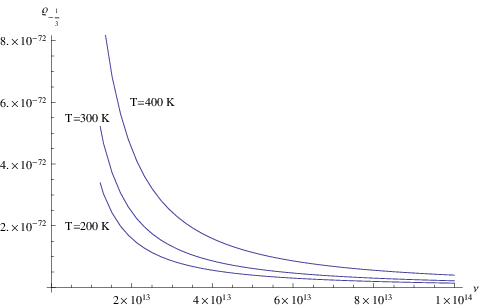
5 Conclusions and remarks: generalized Wien’s law for cosmic string loops and electromagnetic radiation
It has been recalled that the adiabatic theorem shows that in adiabatic reversible processes. From here follows, for instance, that the spectral distribution of should have the general form (3.8), and from here it follows, too, that . In the case of photons (), it follows from here the well-known Wien’s law, with [19].
Here we will comment about the generalization of Wien’s law to the case of cosmic string loops, or for cosmic membranes. Having this generalization may be of interest to relate the temperature of these objects to their microscopic geometrical features.
From , one cannot conclude in general that , as it has been done in Ref. [12], because this is a result for photons (or for systems with proportional to ). In view of (4.1), instead, it is seen that leads to
| (5.1) |
where is the most probable value of the length .
For electromagnetic radiation () this yields indeed . However, for cosmic string loops () the corresponding form is , for cosmic membranes () (5.1) yields , and for dark energy () one has . Thus, having some detailed information on the dispersion relation of the systems with different from is essential to go from the general form to the several particular forms summarized in in terms of the characteristic length. Since in Ref [12] this information was lacking, it was assumed that the form was valid for systems with all values of . In fact the behavior (5.1) is consistent with expansion (2.3) for the entropy. In an expansion, electromagnetic radiation, cools as ( being the length scale factor of the container), whereas the system of cosmic string loops becomes hotter, as .
Second, it is worth to remark that systems with do not seem to follow Planck statistics (nor Bose-Einstein nor Fermi-Dirac ones). This may be related to the fact that they are not stable equilibrium systems, but steady states kept by an external input, which makes them to depend strongly on the particular dynamics, which is reflected in (4.11) through the value of the exponent . This makes even more surprising the fact that even for these systems the energy spectral distribution may be written in the general form (3.8).
One topic of discussion in connection with systems with negative pressure is about the possibility or impossibility of the so-called phantom dark-energy. In the present family of models, phantom dark energy with would lead to a negative entropy. Equation (4.6) gives some more requirements related to the distribution function (4.4), according to which, to have , one should have that the absolute value of should be less than , being the exponent in (4.4). The situation with would then require that , but not much is known about the actual value of . Let us mention that in superfluid turbulence, the exponent describing the length probability distribution of quantized vortices is ; in the hypothetical case that had also this value (this is only meant for the sake of a concrete illustration), the values of consistent with would be . Thus, for the family of systems studied here, the admissible values of are related to their spectral properties (as for instance (4.4) or (4.11)) in a restrictive way.
Acknowledgements
The authors acknowledge the support of the Università di Palermo (Fondi 60% 2012-ATE-0106 and Progetto CoRI 2012, Azione d) and the collaboration agreement between Università di Palermo and Universitàt Autònoma de Barcelona. DJ acknowledges the financial support from the Dirección General de Investigación of the Spanish Ministry of Education under grant FIS2009-13370-C02-01 and of the Direcció General de Recerca of the Generalitat of Catalonia, under grant 2009 SGR-00164. M.S. acknowledges the hospitality of the ”Group of Fisica Estadistica of the Universitàt Autònoma de Barcelona”.
References
- [1] L. Amendola and S. Tsujikawa, Dark energy. Theory and observation (Cambridge University Press, Cambridge, 2010).
- [2] L. Papantonopoulos, ed. The invisible universe: dark matter and dark energy, Lect. Not. Phys. 720, (Springer, Berlin, 2007).
- [3] L.P. Chimento, A.S. Jakubi, D. Pavón, Phys. Rev. D 77 (2003) 083513.
- [4] G. Olivares, F. Atrio-Bavandela and D. Pavón, Phys. Rev. D 77 (2008) 063513.
- [5] Y. Gong, B. Wang and A. Wang, Phys. Rev. D 75 (2007) 123516.
- [6] D. Jou, M.S. Mongiovì and M. Sciacca, Phys. Rev. D 83 (2011) 043519.
- [7] D. Jou, M.S. Mongiovì and M. Sciacca, Phys. Rev. D, 83, 103526 (2011).
- [8] D. Jou, M.S. Mongiovì and M. Sciacca, Studies in thermal and dynamical duality, Boll. Mat. Pura Appl. IV, 115 (Aracne Ed., Roma, 2011).
- [9] A. Abramowski et al., Astropart. Phys. 34, 738 (2011).
- [10] J. Bolmont and A. Jacholkowska, Adv. Space Res. 47,380 (2011).
- [11] J. Albert et al., Phys. Lett. B 668, 253 (2008).
- [12] J. A. S. Lima and J. S. Alcaniz, Phys. Lett. B 600 (2004) 191.
- [13] P. Eherenfest, Philos. Mag. 33 (1917) 500.
- [14] A. Vilenkin and E.P.S. Shelhard, Cosmic strings and other topological defects (Cambridge University Press, Cambridge, 2002).
- [15] J. Polchinski and J.V. Rocha, Phys. Rev. D 74 (2006) 083504.
- [16] S.C. Davis, Phys. Lett. B 645 (2007) 323.
- [17] S.K. Nemirovskii, Phys. Rev. B 77 (2008) 214509.
- [18] D. Jou and M.S. Mongiovì, Phys. Lett. A 373 (2009) 2306.
- [19] L. D. Landau, E. M. Lifshitz, Statistical Physics, (Pergamon Press, Oxford, 1980).