跳到论文正文
W Papers独立论文阅读器 arXiv:1310.6170 论文正文 计算阅读时间 · 0%
引用这篇论文根据当前论文元数据生成,正式投稿前建议核对。


License: arXiv.org perpetual non-exclusive license
arXiv:1310.6170v1 [math.NA] 23 Oct 2013

A Nyström method for a boundary integral equation related to the Dirichlet problem on domains with corners

Luisa Fermo Affiliation: Department of Mathematics and Computer Science Affiliation: University of Cagliari Affiliation: Viale Merello 92, 09123 Cagliari, Italy Affiliation: Concetta Laurita Affiliation: Department of Mathematics, Computer Science and Economics Affiliation: University of Basilicata Affiliation: Via dell’Ateneo Lucano 10, 85100 Potenza, Italy
Abstract

The authors consider the interior Dirichlet problem for Laplace’s equation on planar domains with corners. In order to approximate the solution of the corresponding double layer boundary integral equation, they propose a numerical method of Nyström type, based on a Lobatto quadrature rule. The convergence and stability of the method are proved and some numerical tests are included.

Keywords: Boundary integral equations, Dirichlet problem, Nyström method

Mathematics Subject Classification: 65R20

1 Introduction

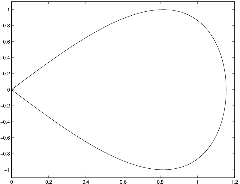
Let DD be a simply connected bounded region in the plane and let its boundary Σ\Sigma be a simple closed piecewise smooth curve. Let us assume Σ\Sigma at least twice continuously differentiable, with the exception of corners at some points P1,…,PnP_{1},\ldots,P_{n}.

We consider the interior Dirichlet problem for Laplace’s equation

{Δ​u​(P)=0,P∈Du⁡(P)=g⁡(P),P∈Σ\left\{\begin{array}[]{ll}\Delta u(P)=0,&\hbox{$P\in D$}\\ u(P)=g(P),&\hbox{$P\in\Sigma$}\end{array}\right. (1)

where gg is a given sufficiently smooth boundary function on Σ\Sigma.

Using a double layer potential representation for the solution of (1)

u⁡(A)=∫Σψ⁡(Q)​∂∂𝐧Q​[log⁡|A−Q|]​d​ΣQ,A∈D,u(A)=\int_{\Sigma}\psi(Q)\frac{\partial}{\partial\mathbf{n}_{Q}}[\log{|A-Q|}]d\Sigma_{Q},\quad A\in D, (2)

with 𝐧Q\mathbf{n}_{Q} the inner normal to Σ\Sigma at QQ, leads to the BIE of the second kind (see, for instance, [1])

(−2​π+Ω⁡(P))​ψ​(P)+∫Σψ⁡(Q)​∂∂𝐧Q​[log⁡|P−Q|]​d​ΣQ=g⁡(P),P∈Σ,(-2\pi+\Omega(P))\psi(P)+\int_{\Sigma}\psi(Q)\frac{\partial}{\partial\mathbf{n}_{Q}}[\log{|P-Q|}]d\Sigma_{Q}=g(P),\quad P\in\Sigma, (3)

whose unknown is the so-called double layer density function ψ⁡(P)\psi(P) and where Ω⁡(P)\Omega(P) denotes the interior angle to Σ\Sigma at PP. Note that Ω⁡(P)=π\Omega(P)=\pi if Σ\Sigma is smooth in PP, while in the “corner points” we assume

0<Ω⁡(P)<2​π.0<\Omega(P)<2\pi.

Defining the operator

(K​ψ)​(P)=(−π+Ω⁡(P))​ψ​(P)+∫Σψ⁡(Q)​∂∂𝐧Q​[log⁡|P−Q|]​d​ΣQ,P∈Σ(K\psi)(P)=(-\pi+\Omega(P))\psi(P)+\int_{\Sigma}\psi(Q)\frac{\partial}{\partial\mathbf{n}_{Q}}[\log{|P-Q|}]d\Sigma_{Q},\quad P\in\Sigma (4)

for ψ∈C⁡(Σ)\psi\in C(\Sigma), one can rewrite equation (3) in the following more compact operator form

(−π+K)​ψ=g.(-\pi+K)\psi=g. (5)

It is well known (see, for instance, [1]) that the operator K{K} is a bounded map from C⁡(Σ)C(\Sigma) into C⁡(Σ)C(\Sigma) and is compact when Σ\Sigma is a smooth curve. On the other hand, KK is no longer compact when the boundary Σ\Sigma is only piecewise smooth, due to the presence of the corner points. In addition, the double layer density function may have a singularity in corners of the type

dβ,β=ππ+|π−ϕ|,d^{\beta},\quad\beta=\frac{\pi}{\pi+|\pi-\phi|},

with dd the distance from the corner and ϕ\phi the interior angle at the corner.

The most popular methods to solve such a problem, for instance collocation, Galerkin and Nyström methods, are based on piecewise polynomial approximations with graded meshes (see, for example, [8, 16, 18, 23] and the references therein). The use of this type of approximation allows, by grading properly the mesh, one to obtain arbitrarily high orders of convergence. Nevertheless, the final linear systems one has to solve become ill-conditioned as the local degree increases.

A different approach is proposed in [22] where the authors describe a method based on a global approximation of the unknown function. By representing the solution of the Dirichlet problem in the form of a single layer potential, they reduce it to solving a system of integral equations of the first kind. Then, after introducing some smoothing changes of variable, they apply a collocation method approximating the unknown density by means of polynomials over each smooth section of the boundary. The numerical results improve as the regularizing parameter increases. Unfortunately, in [22], the stability and convergence of the described numerical procedure are not theoretically proved and error estimates are not given.

More recently an extensive literature on efficient numerical methods to discretize boundary integral equations connected with elliptic problems on domains with corners has been developed (see [3, 4, 5, 6, 7, 14, 15] and the references therein).
In [7] a scheme for the numerical solution of the Neumann problem for the Laplace equation is introduced. The solutions of the standard corresponding integral equations can be unbounded at the corners. In order to achieve high accuracy in the computation of the Nyström solution, the authors propose the analytical subtraction of singularities and a special treatment of nearly non-integrable integrands in such a way as to avoid cancellation errors.
A scheme dubbed “recursive inverse preconditioning” has been introduced in [15] and further developed in [14]. It is a technique which allows to overcome the negative effects of the ill-conditioning of matrices arising from Nyström discretization of singular integral equations on non-smooth domains.
In [3, 4] the author presents a Nyström method based on discretization techniques described in [5] and [6]. The advantage of this method is that, in addition to producing well conditioned linear systems, thanks to a compression scheme, the approach reduces the number of equations which becomes excessively large in the presence of large-scale domains with corners. Nevertheless, in these papers the mathematical analysis of stability and convergence of the proposed procedures is not carried out but are only demonstrated through several numerical examples which show high computational accuracy.

Here we propose a numerical method, based on global approximations, that directly produces well conditioned systems without resorting to preconditioning techniques. By following already known ideas (see [1] and the references therein), we decompose, in a suitable way, the piecewise smooth boundary Σ\Sigma into sections and convert the boundary integral equation (5) into an equivalent system of integral equations of the second kind. Then a Nyström method using a global approximation over each smooth section of the boundary is applied for its numerical solution. The method applies the Lobatto quadrature rule in order to evaluate the integrals involved in the system. In any case, a slight modification of the corresponding discrete operator around the corners is needed in the approximating system to achieve stability. Finally, the solution of the linear system to which the method leads is used to calculate a discrete approximation of the double layer potential (2). We are able to prove theoretically the stability and convergence of the proposed procedure. Moreover, we also show that the linear systems arising from the discretization of the system of boundary integral equations are well conditioned. Neverthless, for domains with a large number of corner points the procedure involves high computational costs as the dimension of the linear system increases.

The contents of the paper are as follows. Section 2 provides preliminary definitions, notations and results. Section 3 is devoted to describing the numerical procedure and to establishing the main theorems about its stability and convergence. Section 4 contains the proofs of the theoretical results and, finally, Section 5 concludes the paper by presenting some numerical tests.

2 Preliminaries

2.1 Function spaces

Let Lp​([0,1])L^{p}([0,1]) be the space of all measurable functions ff on [0,1][0,1] such that

‖f‖p=(∫01|f⁡(x)|p​𝑑x)1p<+∞,1≤p<+∞.\|f\|_{p}=\left(\int_{0}^{1}|f(x)|^{p}dx\right)^{\frac{1}{p}}<+\infty,\quad 1\leq p<+\infty.

With w⁡(x)∈Lp​([0,1])w(x)\in L^{p}([0,1]), a Jacobi weight on [0,1][0,1], we set f∈Lwp​([0,1])f\in L_{w}^{p}([0,1]) if and only if f​w∈Lp​([0,1])fw\in L^{p}([0,1]), 1≤p<+∞1\leq p<+\infty and equip the space Lwp​([0,1])L_{w}^{p}([0,1]) with the norm

‖f​w‖p=(∫01|f⁡(x)​w​(x)|p​𝑑x)1p,1≤p<+∞.\|fw\|_{p}=\left(\int_{0}^{1}|f(x)w(x)|^{p}dx\right)^{\frac{1}{p}},\quad 1\leq p<+\infty.

Moreover, we consider the Sobolev-type subspace Wrp​(w)W^{p}_{r}(w) of Lwp​([0,1])L_{w}^{p}([0,1]) defined as follows

Wrp​(w)={f∈Lwp​([0,1])∣‖f‖Wrp​(w)=‖f​w‖p+‖f(r)​φr​w‖p<∞},W^{p}_{r}(w)=\{f\in L_{w}^{p}([0,1])\ \mid\ \|f\|_{W^{p}_{r}(w)}=\|fw\|_{p}+\|f^{(r)}\varphi^{r}w\|_{p}<\infty\},

where rr is a positive integer and φ⁡(x)=x⁡(1−x)\varphi(x)=\sqrt{x(1-x)}.

Finally, for any r∈ℕ0∪{∞}r\in\mathbb{N}_{0}\cup\{\infty\}, let us consider the following direct product

Cr([0,1])m=Cr​([0,1])×Cr​([0,1])×…×Cr​([0,1])⏟m,C^{r}([0,1])^{{}^{m}}=\underbrace{C^{r}([0,1])\times C^{r}([0,1])\times\ldots\times C^{r}([0,1])}_{m},

which is complete equipped with the norm

‖(f1,f2,…,fm)‖∞=maxi=1,2,…,m⁡‖fi‖∞.\|(f_{1},f_{2},\ldots,f_{m})\|_{\infty}=\max_{i=1,2,\ldots,m}\|f_{i}\|_{\infty}. (6)

2.2 The Lobatto quadrature rule

In this subsection we give some remarks on the well-known Lobatto quadrature rule (see, for instance, [11, p. 104]), since we are going to use a method of Nyström type, based on this integration formula, for the numerical solution of our system of integral equations. Let us premise some notations.

In the sequel 𝒞{\mathcal{C}} denotes a positive constant which may assume different values in different formulas. We write 𝒞=𝒞⁡(a,b,…){\mathcal{C}}={\mathcal{C}}(a,b,...) to say that 𝒞{\mathcal{C}} is dependent on the parameters a,b,….a,b,.... and 𝒞≠𝒞⁡(a,b,…){\mathcal{C}}\neq{\mathcal{C}}(a,b,...) to say that 𝒞{\mathcal{C}} is independent of them. Furthermore, if A,B>0A,B>0 are quantities depending on some parameters, we will write A∼BA\sim B, if there exists a positive constant 𝒞{\mathcal{C}} independent of the parameters of AA and BB such that

1𝒞≤AB≤𝒞.\frac{1}{{\mathcal{C}}}\leq\frac{A}{B}\leq{\mathcal{C}}.

Let w∈Lp​([0,1])w\in L^{p}([0,1]) be a Jacobi weight on [0,1][0,1]. Denoting by ℙm\mathbb{P}_{m} the set of all algebraic polynomials of degree at most mm, for functions f∈Lwpf\in L_{w}^{p}, we define the weighted error of best polynomial approximation as

Em​(f)w,p=infPm∈ℙm‖(f−Pm)​w‖p.E_{m}(f)_{w,p}=\inf_{P_{m}\in\mathbb{P}_{m}}\left\|\left(f-P_{m}\right)w\right\|_{p}.

Moreover, for simplicity, in the case when w⁡(x)≡1w(x)\equiv 1 we set Wrp=Wrp​(w)W^{p}_{r}=W^{p}_{r}(w) and Em​(f)p=Em​(f)w,pE_{m}(f)_{p}=E_{m}(f)_{w,p} .
Now, let {pm​(v1,1)}m\{p_{m}(v^{1,1})\}_{m}, pm​(v1,1)∈ℙmp_{m}(v^{1,1})\in\mathbb{P}_{m}, be the sequence of polynomials which are orthogonal on [0,1][0,1] with respect to the Jacobi weight v1,1​(x)=x⁡(1−x)v^{1,1}(x)=x(1-x). The Lobatto quadrature rule over the interval [0,1][0,1] is given by

∫01f⁡(x)​𝑑x=∑k=0m+1λk​f​(xk)+em​(f)\int_{0}^{1}f(x)dx=\sum_{k=0}^{m+1}\lambda_{k}f(x_{k})+e_{m}(f) (7)

with the nodes x0=0x_{0}=0, x1<x2<…<xmx_{1}<x_{2}<...<x_{m} zeros of pm​(v1,1)p_{m}(v^{1,1}), xm+1=1x_{m+1}=1 and the coefficients

λ0=λm+1=1(m+1)​(m+2),\lambda_{0}=\lambda_{m+1}=\frac{1}{(m+1)(m+2)}, (8)
λk=∫01lk​(x)​v1,1​(x)v1,1​(xk)dx,k=1,…,m,\lambda_{k}=\int_{0}^{1}\frac{l_{k}(x)v^{1,1}(x)}{v^{1,1}(x_{k})}dx,\quad k=1,\ldots,m, (9)

where lk​(x)l_{k}(x) is the kk-th fundamental Lagrange polynomial based on the points x1,…,xmx_{1},\ldots,x_{m}. Finally, em​(f)e_{m}(f) in (7) denotes the remainder term.

The following results give an error estimate for the Lobatto rule (7) in the case when f∈Wr1f\in W^{1}_{r}, r≥1r\geq 1.

Theorem 2.1.

For all f∈W11f\in W^{1}_{1} we have

|em​(f)|≤𝒞m​E2​m​(f′)φ,1|e_{m}(f)|\leq\frac{{\mathcal{C}}}{m}E_{2m}(f^{\prime})_{\varphi,1} (10)

where φ⁡(x)=x⁡(1−x)\varphi(x)=\sqrt{x(1-x)} and 𝒞≠𝒞⁡(m,f){\mathcal{C}}\neq{\mathcal{C}}(m,f).

From the previous theorem and taking into account the Favard inequality (see [12])

Em​(f)w,p≤𝒞mr​Em−r​(f(r))φr​w,p,𝒞≠𝒞⁡(m,f),E_{m}(f)_{w,p}\leq\frac{{\mathcal{C}}}{m^{r}}\,E_{m-r}(f^{(r)})_{\varphi^{r}w,p},\quad{\mathcal{C}}\neq{\mathcal{C}}(m,f), (11)

holding true for each function f∈Wrp​(w)f\in W^{p}_{r}(w), we can immediately deduce the following

Corollary 2.2.

For all f∈Wr1f\in W^{1}_{r}, r≥1r\geq 1, we have

|em​(f)|≤𝒞mr​E2​m+1−r​(f(r))φr,1|e_{m}(f)|\leq\frac{{\mathcal{C}}}{m^{r}}E_{2m+1-r}(f^{(r)})_{\varphi^{r},1} (12)

where φ⁡(x)=x⁡(1−x)\varphi(x)=\sqrt{x(1-x)} and 𝒞≠𝒞⁡(m,f){\mathcal{C}}\neq{\mathcal{C}}(m,f).

3 The method

In this section we are going to propose a method to approximate the solution of the boundary integral equation (5). In order to simplify the presentation, we shall consider the case where the boundary Σ\Sigma has only one corner at a point P0P_{0} with an interior angle ϕ=(1−χ)​π\phi=(1-\chi)\pi, −1<χ<1-1<\chi<1, χ≠0\chi\neq 0. The extension to boundary curves with more than one corner is straightforward.

As recalled in the introduction, in the case under consideration the operator KK in (4) is not compact, but the following splitting of KK is possible ([2, 9, 16])

K=L^+M,K=\hat{L}+M,

with MM a compact operator from C⁡(Σ)C(\Sigma) into C⁡(Σ)C(\Sigma) and L^\hat{L} essentially the so called “wedge operator”, i.e. the operator KK defined on the wedge having vertex at P0P_{0} and arms tangent to those of the boundary Σ\Sigma in the neighborhood of the corner point. The operator L^\hat{L}, which is not compact, satisfies ‖L^‖<π\|\hat{L}\|<\pi. Hence, in the decomposition −π+L^+M-\pi+\hat{L}+M of −π+K-\pi+K, the operator −π+L^-\pi+\hat{L} has a bounded inverse by the Neumann series. Therefore, if −π+L^+M-\pi+\hat{L}+M is injective, the inverse operator (−π+L^+M)−1:C⁡(Σ)→C⁡(Σ)(-\pi+\hat{L}+M)^{-1}:C(\Sigma)\rightarrow C(\Sigma) exists and is bounded. Nevertheless, we don’t apply the Nyström method directly to the initial double layer potential equation

(−π+L^+M)​ψ=g,(-\pi+\hat{L}+M)\psi=g,

since the kernel of the operator MM is bounded but could be discontinuous at the corner point (see [2]) and this would make more difficult the theoretical analysis of the stability and convergence of the numerical procedure.

The method we are going to propose consists of two basic steps. As a first step we decompose, in a suitable way, the curve into sections and reduce (5) to an equivalent system of integral equations. The second step is to apply a numerical method of Nyström type, based on the Lobatto quadrature rule (7), to compute the solution of such a system.

Begin by subdividing Σ\Sigma into the sections Σ1\Sigma_{1}, Σ2\Sigma_{2} and Σ3\Sigma_{3} defined as follows. By proceeding in the counterclockwise direction, let Σ1\Sigma_{1} and Σ2\Sigma_{2} be two sufficiently small smooth arcs of the boundary Σ\Sigma intersecting at the corner P0P_{0}. Moreover, we assume that their lengths are chosen so that Σ1\Sigma_{1} and Σ2\Sigma_{2} essentially coincide with the segments tangent to the curve Σ\Sigma at P0P_{0}, in the sense that

max(x,y)∈Σi|y−yti|≤δ,i=1,2,\max_{(x,y)\in\Sigma_{i}}|y-y_{t_{i}}|\leq\delta,\quad i=1,2, (13)

where ytiy_{t_{i}} denotes the ordinate of the point with abscissa xx on the segment tangent to Σi\Sigma_{i} at P0P_{0} and δ\delta is a very small positive number. Finally, let Σ3\Sigma_{3} be the section connecting Σ1\Sigma_{1} and Σ2\Sigma_{2}.

Then we can rewrite the boundary integral equation (3) as the following system of 33 boundary integral equations

(−2​π+Ω⁡(P))​ψi​(P)+∑j=13∫Σjψj​(Q)​∂∂𝐧Q​[log⁡|P−Q|]​d​ΣQ\displaystyle(-2\pi+\Omega(P))\psi_{i}(P)+\sum_{j=1}^{3}\int_{\Sigma_{j}}\psi_{j}(Q)\frac{\partial}{\partial\mathbf{n}_{Q}}[\log{|P-Q|}]d\Sigma_{Q} =\displaystyle= gi​(P),\displaystyle g_{i}(P), (14)
P∈Σi,i=1,2,3\displaystyle P\in\Sigma_{i},\quad i=1,2,3

where ψi\psi_{i} and gig_{i} denote the restrictions of the functions ψ∈C⁡(Σ)\psi\in C(\Sigma) and g∈C⁡(Σ)g\in C(\Sigma) to the curve Σi\Sigma_{i}, respectively.

In order to transform the above curvilinear 2D integrals into 1D integrals on the same reference interval, let us introduce a parametric representation σi\sigma_{i} defined on the interval [0,1][0,1] for each arc Σi\Sigma_{i}

σi:s∈[0,1]→(ξi​(s),ηi​(s))∈Σi,\sigma_{i}:s\in[0,1]\to(\xi_{i}(s),\eta_{i}(s))\in\Sigma_{i}, (15)

with σi∈C2​([0,1])\sigma_{i}\in C^{2}([0,1]) and |σi′​(s)|≠0|\sigma_{i}^{\prime}(s)|\neq 0 for each 0≤s≤10\leq s\leq 1 and i=1,2,3i=1,2,3. Moreover, without any loss of generality, we assume that σ1′​(s)<0\sigma_{1}^{\prime}(s)<0, σ2′​(s)>0\sigma_{2}^{\prime}(s)>0, σ3′​(s)>0\sigma_{3}^{\prime}(s)>0, ∀s∈[0,1]\forall s\in[0,1], and σ1​(0)=σ2​(0)=P0\sigma_{1}(0)=\sigma_{2}(0)=P_{0}. Then (14) can be rewritten as the following system of integral equations on the interval [0,1][0,1]

(−2π+Ω¯i(s))ψ¯i(s)+∑j=13∫01Ki,j(t,s)ψ¯j(t)dt=g¯i(s),s∈[0,1],i=1,2,3,(-2\pi+\bar{\Omega}_{i}(s))\bar{\psi}_{i}(s)+\sum_{j=1}^{3}\int_{0}^{1}K^{i,j}(t,s)\bar{\psi}_{j}(t)dt=\bar{g}_{i}(s),\quad s\in[0,1],\quad i=1,2,3, (16)

where Ω¯i​(s)=Ω⁡(σi​(s))\bar{\Omega}_{i}(s)=\Omega(\sigma_{i}(s)), ψ¯i​(s)=ψi​(σi​(s))\bar{\psi}_{i}(s)=\psi_{i}(\sigma_{i}(s)), g¯i​(s)=gi​(σi​(s))\bar{g}_{i}(s)=g_{i}(\sigma_{i}(s)) and

Ki,j​(t,s)={ηj′​(t)​[ξi​(s)−ξj​(t)]−ξj′​(t)​[ηi​(s)−ηj​(t)][ξi​(s)−ξj​(t)]2+[ηi​(s)−ηj​(t)]2,i≠jort≠s12​ηj′​(t)​ξj′′​(t)−ξj′​(t)​ηj′′​(t)[ξj′​(t)]2+[ηj′​(t)]2,i=jandt=sK^{i,j}(t,s)=\left\{\begin{array}[]{ll}\displaystyle\frac{\eta^{\prime}_{j}(t)[\xi_{i}(s)-\xi_{j}(t)]-\xi^{\prime}_{j}(t)[\eta_{i}(s)-\eta_{j}(t)]}{[\xi_{i}(s)-\xi_{j}(t)]^{2}+[\eta_{i}(s)-\eta_{j}(t)]^{2}},&\hbox{$i\neq j\quad\mathrm{or}\quad t\neq s$}\\ \\ \displaystyle\frac{1}{2}\frac{\eta^{\prime}_{j}(t)\xi^{\prime\prime}_{j}(t)-\xi_{j}^{\prime}(t)\eta^{\prime\prime}_{j}(t)}{[\xi^{\prime}_{j}(t)]^{2}+[\eta^{\prime}_{j}(t)]^{2}},&\hbox{$i=j\quad\mathrm{and}\quad t=s$}\end{array}\right.

for t,s∈[0,1]t,s\in[0,1]. Note that

Ω¯1​(s)=Ω¯2​(s)={π,0<s≤1(1−χ)​π,s=0\bar{\Omega}_{1}(s)=\bar{\Omega}_{2}(s)=\left\{\begin{array}[]{ll}\pi,&\quad 0<s\leq 1\\ (1-\chi)\pi,&\quad s=0\end{array}\right. (17)

and Ω¯3​(s)=π\bar{\Omega}_{3}(s)=\pi for all s∈[0,1]s\in[0,1].

Now, let us introduce the following complete subspace of the product space C([0,1])3C([0,1])^{{}^{3}} equipped with the norm (6),

𝒳~={(f1,f2,f3)T∈C([0,1])3∣f1(0)=f2(0),f2(1)=f3(0),f1(1)=f3(1)}\tilde{\mathcal{X}}=\left\{(f_{1},f_{2},f_{3})^{T}\in C([0,1])^{{}^{3}}\mid f_{1}(0)=f_{2}(0),\ f_{2}(1)=f_{3}(0),\ f_{1}(1)=f_{3}(1)\right\}

and the bijective map η:C⁡(Σ)→𝒳~\eta:C(\Sigma)\rightarrow\tilde{\mathcal{X}} defined as follows

η​f=(f¯1,f¯2,f¯3),f¯i​(t)=f⁡(σi​(t)),t∈[0,1].\eta f=(\bar{f}_{1},\bar{f}_{2},\bar{f}_{3}),\quad\bar{f}_{i}(t)=f(\sigma_{i}(t)),\quad t\in[0,1].

By defining the following matrices of operators

ℐ=(I000I000I),𝒦=((−π+Ω¯1)​I+𝒦1,1𝒦1,2𝒦1,3𝒦2,1(−π+Ω¯2)​I+𝒦2,2𝒦2,3𝒦3,1𝒦3,2𝒦3,3),{\mathcal{I}}=\left(\begin{array}[]{lll}I&0&0\\ 0&I&0\\ 0&0&I\\ \end{array}\right),\quad\quad{\mathcal{K}}=\left(\begin{array}[]{lll}(-\pi+\bar{\Omega}_{1})I+\mathcal{K}^{1,1}&\mathcal{K}^{1,2}&\mathcal{K}^{1,3}\\ \mathcal{K}^{2,1}&(-\pi+\bar{\Omega}_{2})I+\mathcal{K}^{2,2}&\mathcal{K}^{2,3}\\ \mathcal{K}^{3,1}&\mathcal{K}^{3,2}&\mathcal{K}^{3,3}\\ \end{array}\right), (18)

with II the identity operator on the space C⁡([0,1])C([0,1]) and

(𝒦i,j​ρ)​(s)=∫01Ki,j​(t,s)​ρ​(t)​𝑑t,ρ∈C⁡([0,1]),(\mathcal{K}^{i,j}\rho)(s)=\int_{0}^{1}K^{i,j}(t,s)\rho(t)dt,\quad\rho\in C([0,1]),

the system (16) can be rewritten, in a compact form, as follows

(−π​ℐ+𝒦)​ψ¯=g¯,(-\pi{\mathcal{I}}+{\mathcal{K}})\bar{\psi}=\bar{g}, (19)

where

ψ¯=(ψ¯1,ψ¯2,ψ¯3)T∈𝒳~,g¯=(g¯1,g¯2,g¯3)T∈𝒳~.\bar{\psi}=\left(\bar{\psi}_{1},\bar{\psi}_{2},\bar{\psi}_{3}\right)^{T}\in\tilde{\mathcal{X}},\quad\bar{g}=\left(\bar{g}_{1},\bar{g}_{2},\bar{g}_{3}\right)^{T}\in\tilde{\mathcal{X}}. (20)

Let us observe that the operator (−π​ℐ+𝒦)−1:𝒳~→𝒳~(-\pi{\mathcal{I}}+{\mathcal{K}})^{-1}:\tilde{\mathcal{X}}\rightarrow\tilde{\mathcal{X}} exists and is bounded since we have

(−π​ℐ+𝒦)=η⁡(−π+K)​η−1.(-\pi{\mathcal{I}}+{\mathcal{K}})=\eta(-\pi+K)\eta^{-1}. (21)

Moreover, let us note that the integral operators 𝒦i,j\mathcal{K}^{i,j} are compact on the space C⁡([0,1])C([0,1]), since their kernels are continuous on [0,1]×[0,1][0,1]\times[0,1] (see, for instance, [2, 18]), except when i,j∈{1,2}i,j\in\{1,2\} and i≠ji\neq j. In fact, in such cases 𝒦i,j\mathcal{K}^{i,j} takes the following form (see [2, 9, 16])

(𝒦i,j​ρ)​(s)=(ℒ​ρ)​(s)+(ℳi,j​ρ)​(s),(\mathcal{K}^{i,j}\rho)(s)=(\mathcal{L}\rho)(s)+(\mathcal{M}^{i,j}\rho)(s), (22)

where the integral operator ℒ\mathcal{L} is defined as follows

(ℒ​ρ)​(s)=∫01L⁡(t,s)​ρ​(t)​𝑑t,ρ∈C⁡([0,1]),(\mathcal{L}\rho)(s)=\int_{0}^{1}L(t,s)\rho(t)dt,\quad\rho\in C([0,1]),

with the Mellin–type kernel L⁡(t,s)L(t,s) given by

L⁡(t,s)=−s​sin⁡(χ​π)s2+2​t​s​cos⁡(χ​π)+t2,L(t,s)=-\frac{s\sin{(\chi\pi)}}{s^{2}+2ts\cos{(\chi\pi)}+t^{2}},

and

(ℳi,j​ρ)​(s)=∫01Mi,j​(t,s)​ρ​(t)​𝑑t,ρ∈C⁡([0,1]),(\mathcal{M}^{i,j}\rho)(s)=\int_{0}^{1}M^{i,j}(t,s)\rho(t)dt,\quad\rho\in C([0,1]),

with the kernel Mi,j​(t,s)M^{i,j}(t,s) continuous on [0,1]×[0,1][0,1]\times[0,1].

In order to carry out the theoretical analysis of the stability and convergence of the numerical procedure we are going to propose, we rewrite (19) as follows

(−π​ℐ+𝒲+𝒮)​ψ¯=g¯(-\pi\mathcal{I}+\mathcal{W}+\mathcal{S})\bar{\psi}=\bar{g} (23)

with

𝒲=((−π+Ω¯1)​Iℒ0ℒ(−π+Ω¯2)​I0000){\mathcal{W}}=\left(\begin{array}[]{lll}(-\pi+\bar{\Omega}_{1})I&\mathcal{L}&0\\ \mathcal{L}&(-\pi+\bar{\Omega}_{2})I&0\\ 0&0&0\\ \end{array}\right) (24)

and

𝒮=𝒦−𝒲{\mathcal{S}}={\mathcal{K}}-{\mathcal{W}} (25)

and we introduce the following complete subspace of the product space C([0,1])3C([0,1])^{{}^{3}}

𝒳={(f1,f2,f3)T∈C([0,1])3∣f1(0)=f2(0)}.{\mathcal{X}}=\left\{(f_{1},f_{2},f_{3})^{T}\in C([0,1])^{{}^{3}}\mid f_{1}(0)=f_{2}(0)\right\}. (26)

Note that 𝒳~⊂𝒳\tilde{\mathcal{X}}\subset{\mathcal{X}}. Then we are able to prove the following result concerning the solvability of the system (23) in the spaces 𝒳{\mathcal{X}} and 𝒳~\tilde{\mathcal{X}}.

Theorem 3.1.

Let Ker⁡(−π​ℐ+𝒲+𝒮)={0}\mathrm{Ker}(-\pi\mathcal{I}+{\mathcal{W}}+{\mathcal{S}})=\{0\} in the Banach space 𝒳{\mathcal{X}}. Then system (23)(\ref{sistop1}) has a unique solution in 𝒳{\mathcal{X}} for each given right hand side g¯∈𝒳\bar{g}\in{\mathcal{X}}. Moreover, if g¯∈𝒳~\bar{g}\in\tilde{\mathcal{X}} then the solution ψ¯\bar{\psi} of (23)(\ref{sistop1}) also belongs to 𝒳~\tilde{\mathcal{X}}.

Moreover, it is known that (see [1, 8, 13] and the references therein) even if the Dirichlet data gg is a smooth function, the solution ψ¯=(ψ¯1,ψ¯2,ψ¯3)T\bar{\psi}=\left(\bar{\psi}_{1},\bar{\psi}_{2},\bar{\psi}_{3}\right)^{T} of (23) satisfies the following smoothness properties:

  • •

    ψ¯3\bar{\psi}_{3} is smooth;

  • •

    for i∈{1,2}i\in\{1,2\}

    ψ¯i​(t)=O⁡(tβ),0<t≤1,β=11+|χ|,\bar{\psi}_{i}(t)=O\left(t^{\beta}\right),\quad 0<t\leq 1,\quad\beta=\frac{1}{1+|\chi|}, (27)
    ψ¯i(r)(t)≤𝒞tβ−r,0<t≤1,r=1,2,….\bar{\psi}_{i}^{(r)}(t)\leq{\mathcal{C}}t^{\beta-r},\quad 0<t\leq 1,\quad r=1,2,\ldots\quad. (28)

Therefore, there will almost always be an algebraic singularity in the first derivative of the double layer density function ψ\psi near the corner points, being 12<β<1\frac{1}{2}<\beta<1.

Now, in order to approximate the solution of (19) or, equivalently, of (23), we are going to propose a numerical method of Nyström type based on the Lobatto quadrature rule (7).
Then, for any fixed m∈ℕm\in\mathbb{N}, denoting by λh\lambda_{h} and xhx_{h}, h=0,1,…,m+1h=0,1,\ldots,m+1, the coefficients and the nodes of formula (7), respectively, we define the following finite rank operators

(ℒm​ρ)​(s)=∑h=0m+1λh​L​(xh,s)​ρ​(xh),(\mathcal{L}_{m}\rho)(s)=\sum_{h=0}^{m+1}\lambda_{h}L(x_{h},s)\rho(x_{h}), (29)

approximating ℒ\mathcal{L}, and

(ℳmi,j​ρ)​(s)=∑h=0m+1λh​Mi,j​(xh,s)​ρ​(xh),(\mathcal{M}_{m}^{i,j}\rho)(s)=\sum_{h=0}^{m+1}\lambda_{h}M^{i,j}(x_{h},s)\rho(x_{h}), (30)
(𝒦mi,j​ρ)​(s)=∑h=0m+1λh​Ki,j​(xh,s)​ρ​(xh),(\mathcal{K}_{m}^{i,j}\rho)(s)=\sum_{h=0}^{m+1}\lambda_{h}K^{i,j}(x_{h},s)\rho(x_{h}), (31)

approximating the entries ℳi,j\mathcal{M}^{i,j} and 𝒦i,j\mathcal{K}^{i,j} of the matrix 𝒮\mathcal{S}, respectively.

Now, any sequence of operators {𝒦mi,j}m\left\{\mathcal{K}_{m}^{i,j}\right\}_{m} is pointwise convergent to the operator 𝒦i,j\mathcal{K}^{i,j} in the space C⁡([0,1])C([0,1]), as well as {ℳmi,j​ρ}m\left\{\mathcal{M}_{m}^{i,j}\rho\right\}_{m} tends to ℳi,j​ρ\mathcal{M}^{i,j}\rho for any continuous function ρ\rho on [0,1][0,1]. On the other hand, it is possible to prove that, for a function ρ∈C⁡([0,1])\rho\in C([0,1]), the sequence of functions {ℒm​ρ}m\left\{\mathcal{L}_{m}\rho\right\}_{m} converges uniformly to ℒ​ρ\mathcal{L}\rho in any interval of the type [cm2−2​ϵ,1]\left[\displaystyle\frac{c}{m^{2-2\epsilon}},1\right], for some constant c>0c>0 and arbitrarily small ϵ>0\epsilon>0 (see Lemma 4.2) and does not converge in [0,1][0,1].

Let us introduce the following matrices of operators

𝒲m=((−π+Ω¯1)​Iℒm0ℒm(−π+Ω¯2)​I0000){\mathcal{W}_{m}}=\left(\begin{array}[]{lll}(-\pi+\bar{\Omega}_{1})I&\mathcal{L}_{m}&0\\ \mathcal{L}_{m}&(-\pi+\bar{\Omega}_{2})I&0\\ 0&0&0\\ \end{array}\right) (32)

and

𝒮m=(𝒦m1,1ℳm1,2𝒦m1,3ℳm1,2𝒦m2,2𝒦m2,3𝒦m3,1𝒦m3,2𝒦m3,3).{\mathcal{S}}_{m}=\left(\begin{array}[]{lll}\mathcal{K}_{m}^{1,1}&\mathcal{M}_{m}^{1,2}&\mathcal{K}_{m}^{1,3}\\ \mathcal{M}_{m}^{1,2}&\mathcal{K}_{m}^{2,2}&\mathcal{K}_{m}^{2,3}\\ \mathcal{K}_{m}^{3,1}&\mathcal{K}_{m}^{3,2}&\mathcal{K}_{m}^{3,3}\\ \end{array}\right). (33)

In order to establish stability and convergence results for the procedure we are going to propose, following an idea in [21], we need to slightly modify just 𝒲m{\mathcal{W}}_{m}. More precisely, for a fixed a constant c>0c>0 and an arbitrarily small ϵ>0\epsilon>0, we define

(𝒲~m​ϱ)​(s)={(𝒲m​ϱ)​(s),cm2−2​ϵ≤s≤1m2−2​ϵc​[s⁡(𝒲m​ϱ)​(cm2−2​ϵ)+(cm2−2​ϵ−s)​(𝒲​ϱ)​(0)],0≤s<cm2−2​ϵ(\tilde{\mathcal{W}}_{m}\varrho)(s)=\left\{\begin{array}[]{ll}({\mathcal{W}}_{m}\varrho)(s),&\hbox{$\displaystyle\frac{c}{m^{2-2\epsilon}}\leq s\leq 1$}\\ \\ \displaystyle\frac{m^{2-2\epsilon}}{c}\left[s({\mathcal{W}}_{m}\varrho)\left(\frac{c}{m^{2-2\epsilon}}\right)+\left(\frac{c}{m^{2-2\epsilon}}-s\right)({\mathcal{W}}\varrho)(0)\right],&\hbox{$0\leq s<\displaystyle\frac{c}{m^{2-2\epsilon}}$}\end{array}\right. (34)

with ϱ=(ϱ1,ϱ2,ϱ3)T∈C([0,1])3\varrho=(\varrho_{1},\varrho_{2},\varrho_{3})^{T}\in C([0,1])^{{}^{3}}.

The operators 𝒲~m\tilde{\mathcal{W}}_{m} and 𝒮m{\mathcal{S}}_{m} satisfy the following theorems.

Theorem 3.2.

Let 𝒲{\mathcal{W}} and 𝒲~m\tilde{\mathcal{W}}_{m} be defined in (24)(\ref{MatrixW}) and (34)(\ref{opmodified}), respectively. Then the operators 𝒲~m:𝒳→𝒳\tilde{\mathcal{W}}_{m}:{\mathcal{X}}\to{\mathcal{X}} are linear maps such that

limm→∞‖𝒲~m‖<π\lim_{m\to\infty}\|\tilde{\mathcal{W}}_{m}\|<\pi (35)

and

limm→∞‖(𝒲~m−𝒲)​ρ‖∞=0,∀ρ∈𝒳.\lim_{m\to\infty}\|(\tilde{\mathcal{W}}_{m}-{\mathcal{W}})\rho\|_{\infty}=0,\quad\forall\ \rho\in{\mathcal{X}}. (36)
Theorem 3.3.

Let 𝒮{\mathcal{S}} and 𝒮m{\mathcal{S}_{m}} be defined in (25)(\ref{MatrixS}) and (33)(\ref{MatrixSm}), respectively. Then the operators 𝒮m:𝒳→𝒳{\mathcal{S}}_{m}:{\mathcal{X}}\to{\mathcal{X}} are linear maps such that the set {𝒮m}m\left\{{\mathcal{S}_{m}}\right\}_{m} is collectively compact and

limm→∞‖(𝒮m−𝒮)​ρ‖∞=0,∀ρ∈𝒳.\displaystyle\lim_{m\to\infty}\|({\mathcal{S}}_{m}-{\mathcal{S}}){\rho}\|_{\infty}=0,\quad\forall\ \rho\in{\mathcal{X}}. (37)

The method we are proposing here consists of solving, instead of the system of integral equations (23), the approximating one

(−π​ℐ+𝒲~m+𝒮m)​ψ¯m=g¯,(-\pi\mathcal{I}+\tilde{\mathcal{W}}_{m}+{\mathcal{S}}_{m})\bar{\psi}_{m}=\bar{g}, (38)

whose unknown is the array of functions denoted by ψ¯m=(ψ¯m,1,ψ¯m,2,ψ¯m,3)T\bar{\psi}_{m}=(\bar{\psi}_{m,1},\bar{\psi}_{m,2},\bar{\psi}_{m,3})^{T}.
In order to compute the solution ψ¯m\bar{\psi}_{m} of (38) at the quadrature nodes xlx_{l}, l=0,1,…,m+1l=0,1,\ldots,m+1, let us collocate each equation in these points. In this way we obtain the following linear system of 3​(m+2)3(m+2) equations in the 3​(m+2)3(m+2) unknowns ψ¯m,j​(xl)\bar{\psi}_{m,j}(x_{l}), j=1,2,3j=1,2,3, l=0,1,…,m+1l=0,1,...,m+1

(−πℐ+𝒲~m+𝒮m)ψ¯m(xl)=g¯(xl),l=0,1,…,m+1.(-\pi\mathcal{I}+\tilde{\mathcal{W}}_{m}+{\mathcal{S}}_{m})\bar{\psi}_{m}(x_{l})=\bar{g}(x_{l}),\quad\quad l=0,1,\ldots,m+1. (39)

Rewriting this linear system in the more compact form

Am​𝐚=𝐛,A_{m}\mathbf{a}=\mathbf{b}, (40)

with AmA_{m} the matrix of the coefficients,

𝐚=(a1,0,…,a1,m+1,a2,0,…,a2,m+1,a3,0,…,a3,m+1)\mathbf{a}=\left(a_{1,0},\ldots,a_{1,m+1},a_{2,0},\ldots,a_{2,m+1},a_{3,0},\ldots,a_{3,m+1}\right)

the array of the unknowns and

𝐛=(b1,0,…,b1,m+1,b2,0,…,b2,m+1,b3,0,…,b3,m+1)\mathbf{b}=\left(b_{1,0},\ldots,b_{1,m+1},b_{2,0},\ldots,b_{2,m+1},b_{3,0},\ldots,b_{3,m+1}\right)

the right hand side vector, we see that system (40) is equivalent to the approximating problem (38) (see, for instance, [1, p.101]). More precisely, if ℝ~3​(m+2)\tilde{\mathbb{R}}^{3(m+2)} denotes the subspace of ℝ3​(m+2)\mathbb{R}^{3(m+2)} containing all the arrays

(c1,0,…,c1,m+1,c2,0,…,c2,m+1,c3,0,…,c3,m+1)\left(c_{1,0},\ldots,c_{1,m+1},c_{2,0},\ldots,c_{2,m+1},c_{3,0},\ldots,c_{3,m+1}\right)

such that c1,0=c2,0c_{1,0}=c_{2,0}, we have that each solution ψ¯m∈𝒳\bar{\psi}_{m}\in{\mathcal{X}} of (38) furnishes a solution 𝐚\mathbf{a} of system (40) belonging to ℝ~3​(m+2)\tilde{\mathbb{R}}^{3(m+2)}. It will merely be sufficient to evaluate ψ¯m​(s)\bar{\psi}_{m}(s) at the nodes of the Lobatto formula. Viceversa, if 𝐚∈ℝ~3​(m+2)\mathbf{a}\in\tilde{\mathbb{R}}^{3(m+2)} is a solution of (40), there is a unique ψ¯m​(s)∈𝒳\bar{\psi}_{m}(s)\in{\mathcal{X}} which is solution of (38) such that

ψ¯m,i(xl)=ai,l,i=1,2,3,l=0,1,…,m+1.\bar{\psi}_{m,i}(x_{l})=a_{i,l},\quad i=1,2,3,\quad l=0,1,\ldots,m+1. (41)

Then we can conclude that the operator −π​ℐ+𝒲~m+𝒮m-\pi\mathcal{I}+\tilde{\mathcal{W}}_{m}+{\mathcal{S}}_{m} is invertible on the space 𝒳\mathcal{X} if and only if the matrix AmA_{m} is invertible on ℝ~3​(m+2)\tilde{\mathbb{R}}^{3(m+2)}.

Before establishing our main result, let us make some remarks.
The first one concerns the computation of the entries of AmA_{m}. Note that, in order to construct this matrix, one has to calculate the quantities λh​L​(xh,xl)\lambda_{h}L(x_{h},x_{l}). The worst case could occur in the evaluation of λ0​L​(x0,x1)\lambda_{0}L(x_{0},x_{1}) because the values L⁡(x0,x1)L(x_{0},x_{1}) increase more and more as well as mm increases. Nevertheless, since λ0∼1m2\lambda_{0}\sim\displaystyle\frac{1}{m^{2}} (see (8)) and, using x1−x0∼1m2x_{1}-x_{0}\sim\displaystyle\frac{1}{m^{2}} (see (48)), it is easily seen that L⁡(x0,x1)∼m2L(x_{0},x_{1})\sim m^{2} (with the constants in ∼\sim independent of mm), one has that the products λ0​L​(x0,x1)\lambda_{0}L(x_{0},x_{1}) are uniformly bounded with respect to mm.
As a second remark we would like to point out that, for the sake of simplicity, we have used the same number m+2m+2 of quadrature nodes for the Lobatto formula in (29)-(30) and (31). Nevertheless, one can generalize the proposed procedure by using also different numbers of quadrature knots on each smooth arc of the boundary Σj\Sigma_{j}, j=1,2,3j=1,2,3.

Theorem 3.4.

Let Σ∖{P0}\Sigma\setminus\{P_{0}\} of class C2C^{2}. Assume that Ker​{−π​ℐ+𝒲+𝒮}={0}\mathrm{Ker}\{-\pi\mathcal{I}+{\mathcal{W}}+{\mathcal{S}}\}=\{0\} in the space 𝒳{\mathcal{X}}. Then, for sufficiently large mm, say m≥m0m\geq m_{0}, the operators −π​ℐ+𝒲~m+𝒮m-\pi\mathcal{I}+\tilde{\mathcal{W}}_{m}+{\mathcal{S}}_{m} are invertible and their inverses are uniformly bounded on 𝒳{\mathcal{X}}. Moreover, for all g¯∈𝒳∩Cp([0,1])3\bar{g}\in{\mathcal{X}}\cap C^{p}([0,1])^{{}^{3}} with pp large enough, the solutions ψ¯\bar{\psi} of equation (23)(\ref{sistop1}) and ψ¯m\bar{\psi}_{m} of (38)(\ref{sistapprox}), satisfy the following error estimate

‖(ψ¯−ψ¯m)​(s)‖∞≤𝒞⁡[‖(𝒲~m−𝒲)​ψ¯​(s)‖∞+‖(𝒮m−𝒮)​ψ¯​(s)‖∞],𝒞≠𝒞⁡(m),\|(\bar{{\psi}}-\bar{{\psi}}_{m})(s)\|_{\infty}\leq{\mathcal{C}}[\|(\tilde{\mathcal{W}}_{m}-{\mathcal{W}})\bar{{\psi}}(s)\|_{\infty}+\|({{\mathcal{S}}}_{m}-{\mathcal{S}})\bar{{\psi}}(s)\|_{\infty}],\quad{\mathcal{C}}\neq{\mathcal{C}}(m), (42)

where

‖(𝒲~m−𝒲)​ψ¯​(s)‖∞≤{𝒞​max⁡{(1m2−2​ϵ)β,1m1+ϵ},s∈[0,cm2−2​ϵ]𝒞m2​1s12,s∈[cm2−2​ϵ,1],\|(\tilde{\mathcal{W}}_{m}-{\mathcal{W}})\bar{{\psi}}(s)\|_{\infty}\leq\left\{\begin{array}[]{ll}{\mathcal{C}}\max\left\{\left(\displaystyle\frac{1}{m^{2-2\epsilon}}\right)^{\beta},\displaystyle\frac{1}{m^{1+\epsilon}}\right\},&s\in\left[0,\displaystyle\frac{c}{m^{2-2\epsilon}}\right]\\ \displaystyle\frac{{\mathcal{C}}}{m^{2}}\frac{1}{s^{\frac{1}{2}}},&s\in\left[\displaystyle\frac{c}{m^{2-2\epsilon}},1\right]\end{array}\right., (43)

with ϵ\epsilon as in (34)(\ref{opmodified}) and β=11+|χ|\displaystyle\beta=\frac{1}{1+|\chi|}.

Let us remark that (see Theorem 3.3)

limm‖(𝒮m−𝒮)​ψ¯​(s)‖∞=0,∀s∈[0,1]\lim_{m}\|({{\mathcal{S}}}_{m}-{\mathcal{S}})\bar{{\psi}}(s)\|_{\infty}=0,\quad\forall s\in[0,1]

and the rate of convergence depends on the smoothness of the boundary Σ∖{P0}\Sigma\setminus\{P_{0}\} as well as on the behavior of the functions ψ¯j\bar{\psi}_{j} on the interval [0,1][0,1] (see (27), (28)).

Moreover, we can prove the following theorem.

Theorem 3.5.

Denoting by cond⁡(−π​ℐ+𝒲~m+𝒮m)\mathrm{cond}(-\pi\mathcal{I}+\tilde{\mathcal{W}}_{m}+{\mathcal{S}}_{m}) the condition number of the operator −π​ℐ+𝒲~m+𝒮m:𝒳→𝒳-\pi\mathcal{I}+\tilde{\mathcal{W}}_{m}+{\mathcal{S}}_{m}:{\mathcal{X}}\rightarrow{\mathcal{X}} and by cond⁡(Am)\mathrm{cond}(A_{m}) the condition number of the matrix Am:ℝ~3​(m+2)→ℝ~3​(m+2)A_{m}:\tilde{\mathbb{R}}^{3(m+2)}\rightarrow\tilde{\mathbb{R}}^{3(m+2)} in infinity norm, we have that, for any m≥m0m\geq m_{0},

cond⁡(Am)≤cond⁡(−π​ℐ+𝒲~m+𝒮m)≤𝒞,\mathrm{cond}(A_{m})\leq\mathrm{cond}(-\pi\mathcal{I}+\tilde{\mathcal{W}}_{m}+{\mathcal{S}}_{m})\leq{\mathcal{C}}, (44)

where 𝒞≠𝒞⁡(m){\mathcal{C}}\neq{\mathcal{C}}(m).

According to the decomposition of the boundary Σ\Sigma and to the parametric representation (15) introduced of each arc Σi\Sigma_{i}, the double layer potential uu defined by (2), solution of the Dirichlet problem (1), can be rewritten as

u⁡(x,y)=∑i=13∫01Hi​(x,y,t)​ψi¯​(t)​𝑑t,∀(x,y)∈Du(x,y)=\sum_{i=1}^{3}\int_{0}^{1}H_{i}(x,y,t)\bar{\psi_{i}}(t)dt,\quad\forall\ (x,y)\in D (45)

where ψ¯i=ψi∘σi\bar{\psi}_{i}=\psi_{i}\circ\sigma_{i}, with ψi\psi_{i} the double layer density function on Σi\Sigma_{i}, and

Hi​(x,y,t)=ηi′​(t)​[x−ξi​(t)]−ξi′​(t)​[y−ηi​(t)][x−ξi​(t)]2+[y−ηi​(t)]2.H_{i}(x,y,t)=\frac{\eta^{\prime}_{i}(t)[x-\xi_{i}(t)]-\xi^{\prime}_{i}(t)[y-\eta_{i}(t)]}{[x-\xi_{i}(t)]^{2}+[y-\eta_{i}(t)]^{2}}.

Now we propose to approximate the double layer potential u⁡(x,y)u(x,y) in (45) by means of the following function

um​(x,y)=∑i=13∑h=0m+1λh​Hi​(x,y,xh)​ψ¯m,i​(xh),u_{m}(x,y)=\sum_{i=1}^{3}\sum_{h=0}^{m+1}\lambda_{h}H_{i}(x,y,x_{h})\bar{\psi}_{m,i}(x_{h}), (46)

obtained by replacing each function ψi¯\bar{\psi_{i}} on the right-hand side in (45) with the corresponding Nyström interpolant ψ¯m,i\bar{\psi}_{m,i} (ii-th component of the solution ψ¯m\bar{\psi}_{m} of (38)) and, then, by approximating all the integrals using the Lobatto quadrature rule (7) on m+2m+2 points. Let us observe that the values ψ¯m,i​(xh)\bar{\psi}_{m,i}(x_{h}) involved in the formula (46) are just the solutions of the linear system (39).

Theorem 3.6.

For any (x,y)∈D(x,y)\in D, the double layer potential uu defined by (2)(\ref{double}), solution of the Dirichlet problem (1)(\ref{Dirichlet}), and the function umu_{m} given by (46) satisfy the following pointwise error estimate

|u⁡(x,y)−um​(x,y)|≤𝒞m​(1d2+1d)+𝒞′d​‖ψ¯−ψ¯m‖∞,|u(x,y)-u_{m}(x,y)|\leq\frac{{\mathcal{C}}}{m}\left(\frac{1}{d^{2}}+\frac{1}{d}\right)+\frac{{\mathcal{C}}^{\prime}}{d}\left\|\bar{\psi}-\bar{\psi}_{m}\right\|_{\infty}, (47)

where d=mini=1,2,3⁡did=\displaystyle\min_{i=1,2,3}d_{i}, with di=min0≤t≤1⁡|(x,y)−(ξi​(t),ηi​(t))|d_{i}=\displaystyle\min_{0\leq t\leq 1}|(x,y)-(\xi_{i}(t),\eta_{i}(t))|, and 𝒞{\mathcal{C}}, 𝒞′{\mathcal{C}}^{\prime} are positive constants independent of (x,y)(x,y) and mm.

Let us observe that the first addendum on the right hand side of (47) could converge to zero with rate greater than 1/m1/m if the boundary Σ∖P0\Sigma\setminus P_{0} is (q+2)(q+2)-times differentiable, for some q>0q>0. Moreover, from the previous estimate, we can deduce that the error becomes smaller and smaller as well as the point (x,y)∈D(x,y)\in D moves away from the boundary Σ\Sigma.

4 Proofs

In order to prove Theorem 2.1 we need the following result (see [24]).

Lemma 4.1.

Let xkx_{k} and λk\lambda_{k}, k=0,1,…,m+1k=0,1,\ldots,m+1, be the nodes and the coefficients of the quadrature rule defined in (7)(\ref{lobatto}), respectively. Then, setting Δ​xk=xk+1−xk\Delta x_{k}=x_{k+1}-x_{k}, k=0,1,…,mk=0,1,\ldots,m, one has

Δ​xk∼{xk+1​(1−xk+1)m,k=0xk​(1−xk)m,k=1,…,m.\Delta x_{k}\sim\left\{\begin{array}[]{ll}\displaystyle\frac{\sqrt{x_{k+1}(1-x_{k+1})}}{m},&k=0\\ \displaystyle\frac{\sqrt{x_{k}(1-x_{k})}}{m},&k=1,\ldots,m.\end{array}\right. (48)

and

λk∼{Δ​xk,k=0,1,…,mΔ​xk−1,k=m+1.\lambda_{k}\sim\left\{\begin{array}[]{ll}\Delta x_{k},&k=0,1,\ldots,m\\ \Delta x_{k-1},&k=m+1.\end{array}\right. (49)
Proof.

of Theorem 2.1 We can proceed analogously to the proof of Theorem 5.1.8 in [20]. Then, it will be sufficient to prove the following inequality

∑k=0m+1λk​|f⁡(xk)|≤𝒞⁡(‖f‖1+1m​‖f′​φ‖1).\sum_{k=0}^{m+1}\lambda_{k}|f(x_{k})|\leq{\mathcal{C}}\left(\|f\|_{1}+\frac{1}{m}\|f^{\prime}\varphi\|_{1}\right). (50)

Indeed, since the Lobatto quadrature rule is exact for polynomials of degree at most 2​m+12m+1, for any P∈ℙ2​m+1P\in\mathbb{P}_{2m+1} we can write

|em​(f)|≤∫01|f⁡(x)−P⁡(x)​|𝑑x+∑k=0m+1λk|​f​(xk)−P⁡(xk)|.|e_{m}(f)|\leq\int_{0}^{1}|f(x)-P(x)|dx+\sum_{k=0}^{m+1}\lambda_{k}|f(x_{k})-P(x_{k})|. (51)

Hence, by applying (50) and the following inequality ([19])

‖(f−P)′​φ‖1≤𝒞⁡(2​m+1)​‖f−P‖1+E2​m​(f′)φ,1,\|(f-P)^{\prime}\varphi\|_{1}\leq{\mathcal{C}}(2m+1)\|f-P\|_{1}+E_{2m}(f^{\prime})_{\varphi,1}, (52)

we have

|em​(f)|\displaystyle|e_{m}(f)| ≤𝒞⁡[‖f−P‖1+1m​‖(f−P)′​φ‖1]\displaystyle\leq{\mathcal{C}}\left[\|f-P\|_{1}+\frac{1}{m}\|(f-P)^{\prime}\varphi\|_{1}\right]
≤𝒞⁡[‖f−P‖1+1m​E2​m​(f′)φ,1]\displaystyle\leq{\mathcal{C}}\left[\|f-P\|_{1}+\frac{1}{m}E_{2m}(f^{\prime})_{\varphi,1}\right]

from which, by taking the infimum on P∈ℙ2​m+1P\in\mathbb{P}_{2m+1} and using (11), we obtain

|em​(f)|\displaystyle|e_{m}(f)| ≤\displaystyle\leq 𝒞⁡[E2​m+1​(f)1+1m​E2​m​(f′)φ,1]\displaystyle{\mathcal{C}}\left[E_{2m+1}(f)_{1}+\frac{1}{m}E_{2m}(f^{\prime})_{\varphi,1}\right]
≤\displaystyle\leq 𝒞m​E2​m​(f′)φ,1\displaystyle\frac{{\mathcal{C}}}{m}E_{2m}(f^{\prime})_{\varphi,1}

i.e. the thesis.

In order to prove (50) we note that, in virtue of Lemma 4.1, we can write

∑k=0m+1λk​|f⁡(xk)|≤𝒞​∑k=0m+1Δ​xk​|f⁡(xk)|,\sum_{k=0}^{m+1}\lambda_{k}|f(x_{k})|\leq{\mathcal{C}}\sum_{k=0}^{m+1}\Delta x_{k}|f(x_{k})|, (53)

where we set Δ​xm+1=Δ​xm\Delta x_{m+1}=\Delta x_{m}. Then we apply the first one of the following inequalities

(b−a)​|f⁡(a)|(b−a)​|f⁡(b)|}≤[∫ab|f⁡(t)|​𝑑t+(b−a)​∫ab|f′​(t)|​𝑑t]\left.\begin{array}[]{ll}(b-a)|f(a)|\\ (b-a)|f(b)|\end{array}\right\}\leq\left[\int_{a}^{b}|f(t)|dt+(b-a)\int_{a}^{b}|f^{\prime}(t)|dt\right] (54)

with a=xka=x_{k} and b=xk+1b={x_{k+1}} in order to estimate the terms on the right hand side of (53) with k=0,1,…,mk=0,1,\ldots,m and we have

Δ​xk​|f⁡(xk)|\displaystyle\Delta x_{k}|f(x_{k})| ≤\displaystyle\leq [∫xkxk+1|f⁡(x)|​𝑑x+Δ​xk​∫xkxk+1|f′​(x)|​𝑑x]\displaystyle\left[\int_{x_{k}}^{x_{k+1}}|f(x)|dx+\Delta x_{k}\int_{x_{k}}^{x_{k+1}}|f^{\prime}(x)|dx\right] (55)
≤\displaystyle\leq 𝒞⁡[∫xkxk+1|f⁡(x)|​𝑑x+1m​∫xkxk+1|(f′​φ)​(x)|​𝑑x]\displaystyle{\mathcal{C}}\left[\int_{x_{k}}^{x_{k+1}}|f(x)|dx+\frac{1}{m}\int_{x_{k}}^{x_{k+1}}|(f^{\prime}\varphi)(x)|dx\right]

being, for x∈[xk,xk+1]x\in[x_{k},x_{k+1}], xk∼x∼xk+1x_{k}\sim x\sim x_{k+1} and 1−xk∼1−x∼1−xk+11-x_{k}\sim 1-x\sim 1-x_{k+1}.
For the term k=m+1k=m+1, we can apply the second inequality of (54) and obtain

Δ​xm+1|f⁡(xm+1)|≤𝒞⁡[∫xmxm+1|f⁡(x)|​𝑑x+1m​∫xmxm+1|(f′​φ)​(x)|​𝑑x].\Delta x_{m+1}|f(x_{m+1})|\leq{\mathcal{C}}\left[\int_{x_{m}}^{x_{m+1}}|f(x)|dx+\frac{1}{m}\int_{x_{m}}^{x_{m+1}}|(f^{\prime}\varphi)(x)|dx\right]. (56)

Finally, summing up on k=0,1,…,m+1k=0,1,...,m+1 inequalities (55)-(56), we can deduce (50).   ∎

Proof.

of Theorem 3.1 We first prove that 𝒲:𝒳→𝒳{\mathcal{W}}:{\mathcal{X}}\rightarrow{\mathcal{X}} is a bounded operator and satisfies

‖𝒲‖<π.\|{\mathcal{W}}\|<\pi. (57)

From well known results (see, for instance, [1, p. 393]) it follows that for any array of functions ρ=(ρ1,ρ2,ρ3)T∈𝒳\rho=(\rho_{1},\rho_{2},\rho_{3})^{T}\in{\mathcal{X}} one has that 𝒲ρ∈C([0,1])3{\mathcal{W}}\rho\in C([0,1])^{{}^{3}}. Moreover, it is easy to see that 𝒲​ρ∈𝒳{\mathcal{W}}\rho\in{\mathcal{X}} and if ‖ρ‖∞≤1\|\rho\|_{\infty}\leq 1,

‖𝒲​ρ‖∞≤|χ|​π<π.\|{\mathcal{W}}\rho\|_{\infty}\leq|\chi|\pi<\pi.

Therefore, since, for ℐ:𝒳→𝒳\mathcal{I}:{\mathcal{X}}\to{\mathcal{X}}, ‖−π​ℐ‖=π\|-\pi\mathcal{I}\|=\pi, by applying the geometric series theorem we deduce that (−π​ℐ+𝒲)−1(-\pi\mathcal{I}+{\mathcal{W}})^{-1} exists and is a bounded operator on 𝒳{\mathcal{X}} into 𝒳{\mathcal{X}} with

‖(−π​ℐ+𝒲)−1‖≤1π−‖𝒲‖.\|(-\pi\mathcal{I}+{\mathcal{W}})^{-1}\|\leq\frac{1}{\pi-\|{\mathcal{W}}\|}.

Consequently, we can reformulate equation (23) as

ψ¯+(−π​ℐ+𝒲)−1​𝒮​ψ¯=(−π​ℐ+𝒲)−1​g¯.\bar{\psi}+(-\pi\mathcal{I}+{\mathcal{W}})^{-1}{\mathcal{S}}\bar{\psi}=(-\pi\mathcal{I}+{\mathcal{W}})^{-1}\bar{g}. (58)

Now, let us note that the operator 𝒮{\mathcal{S}} also maps 𝒳{\mathcal{X}} into 𝒳{\mathcal{X}} and it is compact since it is a matrix of compact operators. Hence (−π​ℐ+𝒲)−1​𝒮(-\pi\mathcal{I}+{\mathcal{W}})^{-1}{\mathcal{S}} is a compact operator, too. Thus for equation (58) the Fredholm alternative holds true and from the hypothesis it follows that the system (23) is unisolvent in 𝒳{\mathcal{X}} for each right-hand side g¯∈𝒳\bar{g}\in{\mathcal{X}}.
In particular, if g¯∈𝒳~\bar{g}\in\tilde{\mathcal{X}} then the vector ψ¯=(−π​ℐ+𝒲+𝒮)−1​g¯\bar{\psi}=(-\pi\mathcal{I}+{\mathcal{W}}+{\mathcal{S}})^{-1}\bar{g} also belongs to the subspace 𝒳~\tilde{\mathcal{X}}. In fact, since the operator −π​ℐ+𝒲+𝒮=−π+𝒦-\pi\mathcal{I}+{\mathcal{W}}+{\mathcal{S}}=-\pi+\mathcal{K} is invertible in 𝒳~\tilde{\mathcal{X}} (see (21)), there exists an array φ¯∈𝒳~⊂𝒳\bar{\varphi}\in\tilde{\mathcal{X}}\subset{\mathcal{X}} such that φ¯=(−π​ℐ+𝒲+𝒮)−1​g¯\bar{\varphi}=(-\pi\mathcal{I}+{\mathcal{W}}+{\mathcal{S}})^{-1}\bar{g}. Then, by the assumption ψ¯=φ¯\bar{\psi}=\bar{\varphi} follows. ∎

In order to be able to prove Theorem 3.2 we need to prove the following two lemmas.

Lemma 4.2.

Let

L⁡(t,s)=−s​sin⁡(χ​π)s2+2​t​s​cos⁡(χ​π)+t2,t,s∈[0,1],L(t,s)=-\frac{s\sin{(\chi\pi)}}{s^{2}+2ts\cos{(\chi\pi)}+t^{2}},\quad t,s\in[0,1],

for some χ∈ℝ\chi\in\mathbb{R}, |χ|<−1|\chi|<-1, and let eme_{m} be the functional defined as in (7)(\ref{lobatto}). Then, for each s∈(0,1]s\in(0,1] one has

em​(L⁡(⋅,s))≤𝒞​r!mr​1sr/2,e_{m}(L(\cdot,s))\leq{\mathcal{C}}\frac{r!}{m^{r}}\frac{1}{s^{r/2}},

where r∈ℕr\in\mathbb{N} and 𝒞≠𝒞⁡(m){\mathcal{C}}\neq{\mathcal{C}}(m).

Proof.

At first let us note that

L⁡(t,s)=−12​i​[1t+e−i​χ​π​s−1t+ei​χ​π​s],L(t,s)=-\frac{1}{2i}\left[\frac{1}{t+e^{-i\chi\pi}s}-\frac{1}{t+e^{i\chi\pi}s}\right],

from which, for any fixed integer rr, we have

∂r∂tr​L​(t,s)\displaystyle\frac{\partial^{r}}{\partial t^{r}}L(t,s) =\displaystyle= −12​i​[(−1)r​r!(t+e−i​χ​π​s)r+1−(−1)r​r!(t+ei​χ​π​s)r+1]\displaystyle-\frac{1}{2i}\left[\frac{(-1)^{r}r!}{(t+e^{-i\chi\pi}s)^{r+1}}-\frac{(-1)^{r}r!}{(t+e^{i\chi\pi}s)^{r+1}}\right]
=\displaystyle= −(−1)r​r!2​i​(t+ei​χ​π​s)r+1−(t+e−i​χ​π​s)r+1[(t+e−i​χ​π​s)​(t+ei​χ​π​s)]r+1\displaystyle-\frac{(-1)^{r}r!}{2i}\frac{(t+e^{i\chi\pi}s)^{r+1}-(t+e^{-i\chi\pi}s)^{r+1}}{\left[(t+e^{-i\chi\pi}s)(t+e^{i\chi\pi}s)\right]^{r+1}}
=\displaystyle= −(−1)r​r!2​i​[∑k=0r+1(r+1k)​tk​sr+1−k​[ei​χ​π​(r+1−k)−e−i​χ​π​(r+1−k)](t2+2​t​s​cos⁡χ​π+s2)r+1]\displaystyle-\frac{(-1)^{r}r!}{2i}\left[\frac{\displaystyle\sum_{k=0}^{r+1}\left(\begin{array}[]{c}r+1\\ k\end{array}\right)t^{k}s^{r+1-k}[e^{i\chi\pi(r+1-k)}-e^{-i\chi\pi(r+1-k)}]}{(t^{2}+2ts\cos{\chi\pi}+s^{2})^{r+1}}\right]
=\displaystyle= −(−1)r​r!​[∑k=0r+1(r+1k)​tk​sr+1−k​sin⁡(χ​π​(r+1−k))(t2+2​t​s​cos⁡χ​π+s2)r+1].\displaystyle-(-1)^{r}r!\left[\frac{\displaystyle\sum_{k=0}^{r+1}\left(\begin{array}[]{c}r+1\\ k\end{array}\right)t^{k}s^{r+1-k}\sin{(\chi\pi(r+1-k))}}{(t^{2}+2ts\cos{\chi\pi}+s^{2})^{r+1}}\right].

Then

|∂r∂tr​L​(t,s)|\displaystyle\left|\frac{\partial^{r}}{\partial t^{r}}L(t,s)\right| ≤\displaystyle\leq r!​|∑k=0r+1(r+1k)​tk​sr+1−k|(t2+2​t​s​cos⁡χ​π+s2)r+1\displaystyle r!\frac{\left|\displaystyle\sum_{k=0}^{r+1}\left(\begin{array}[]{c}r+1\\ k\end{array}\right)t^{k}s^{r+1-k}\right|}{(t^{2}+2ts\cos{\chi\pi}+s^{2})^{r+1}}
=\displaystyle= r!​(t+s)r+1(t2+2​t​s​cos⁡χ​π+s2)r+1\displaystyle r!\frac{(t+s)^{r+1}}{(t^{2}+2ts\cos{\chi\pi}+s^{2})^{r+1}}

and, consequently,

‖∂r∂tr​L​(⋅,s)​φr‖1\displaystyle\left\|\frac{\partial^{r}}{\partial t^{r}}L(\cdot,s)\varphi^{r}\right\|_{1} =\displaystyle= ∫01|∂r∂tr​L​(t,s)|​φr​(t)​𝑑t\displaystyle\int_{0}^{1}\left|\frac{\partial^{r}}{\partial t^{r}}L(t,s)\right|\varphi^{r}(t)dt
≤\displaystyle\leq r!​∫01(t+s)r+1​tr/2(t2+2​t​s​cos⁡χ​π+s2)r+1​𝑑t.\displaystyle r!\int_{0}^{1}\frac{(t+s)^{r+1}t^{r/2}}{(t^{2}+2ts\cos{\chi\pi}+s^{2})^{r+1}}dt.

Now, setting t=s​xt=sx, we can deduce

‖∂r∂tr​L​(⋅,s)​φr‖1\displaystyle\left\|\frac{\partial^{r}}{\partial t^{r}}L(\cdot,s)\varphi^{r}\right\|_{1} ≤\displaystyle\leq r!sr/2​∫01/s(x+1)r+1​xr/2(x2+2​x​cos⁡χ​π+1)r+1​𝑑x\displaystyle\frac{r!}{s^{r/2}}\int_{0}^{1/s}\frac{(x+1)^{r+1}x^{r/2}}{(x^{2}+2x\cos{\chi\pi}+1)^{r+1}}dx (64)
≤\displaystyle\leq r!sr/2​∫0∞(x+1)r+1​xr/2(x2+2​x​cos⁡χ​π+1)r+1​𝑑x≤𝒞​r!sr/2.\displaystyle\frac{r!}{s^{r/2}}\int_{0}^{\infty}\frac{(x+1)^{r+1}x^{r/2}}{(x^{2}+2x\cos{\chi\pi}+1)^{r+1}}dx\leq{\mathcal{C}}\frac{r!}{s^{r/2}}.

Thus, by applying Corollary 2.2, for r∈ℕr\in\mathbb{N}, it results

|em​(L⁡(⋅,s))|≤𝒞mr​E2​m+1−r​(∂r∂tr​L​(⋅,s))φr,1≤𝒞mr​‖∂r∂tr​L​(⋅,s)​φr‖1|e_{m}(L(\cdot,s))|\leq\frac{{\mathcal{C}}}{m^{r}}E_{2m+1-r}\left(\frac{\partial^{r}}{\partial t^{r}}L(\cdot,s)\right)_{\varphi^{r},1}\leq\frac{{\mathcal{C}}}{m^{r}}\left\|\frac{\partial^{r}}{\partial t^{r}}L(\cdot,s)\varphi^{r}\right\|_{1} (65)

and, combining (65) with (64), the thesis follows. ∎

Lemma 4.3.

Let 𝒳{\mathcal{X}} be the space of functions defined in (26)(\ref{space}) and

ℙ~3=ℙ3∩𝒳\tilde{\mathbb{P}}^{{}^{3}}=\mathbb{P}^{{}^{3}}\cap{\mathcal{X}} (66)

where ℙ\mathbb{P} is the set of all polynomials on [0,1][0,1]. Then ℙ~3\tilde{\mathbb{P}}^{{}^{3}} is a dense subspace in 𝒳{\mathcal{X}}.

Proof.

First, let us prove that ℙ~3¯⊆𝒳\overline{\tilde{\mathbb{P}}^{{}^{3}}}\subseteq{\mathcal{X}} (ℙ~3¯\overline{\tilde{\mathbb{P}}^{{}^{3}}} denoting the closure of ℙ~3\tilde{\mathbb{P}}^{{}^{3}}).
Let φ=(φ1,φ2,φ3)∈ℙ~3¯\varphi=(\varphi_{1},\varphi_{2},\varphi_{3})\in\overline{\tilde{\mathbb{P}}^{{}^{3}}} and {pm}m\{p_{m}\}_{m}, with pm=(pm,1,pm,2,pm,3)∈ℙ~3p_{m}=(p_{m,1},p_{m,2},p_{m,3})\in\tilde{\mathbb{P}}^{{}^{3}}, be a sequence convergent to φ\varphi. Then

limmpm,i=φi,∀i∈{1,2,3}\lim_{m}p_{m,i}=\varphi_{i},\quad\forall i\in\{1,2,3\}

and, consequently, one has φ∈𝒳\varphi\in{\mathcal{X}} since

φ1​(0)=limmpm,1​(0)=limmpm,2​(0)=φ2​(0).\varphi_{1}(0)=\lim_{m}p_{m,1}(0)=\lim_{m}p_{m,2}(0)=\varphi_{2}(0).

Viceversa, we are going to prove that 𝒳⊆ℙ~3¯{\mathcal{X}}\subseteq\overline{\tilde{\mathbb{P}}^{{}^{3}}}. Since ℙ3\mathbb{P}^{{}^{3}} is a dense subspace of the space C([0,1])3C([0,1])^{{}^{3}}, for a given φ=(φ1,φ2,φ3)∈𝒳\varphi=(\varphi_{1},\varphi_{2},\varphi_{3})\in{\mathcal{X}} there exists a sequence {pm}m\{p_{m}\}_{m}, with pm=(pm,1,pm,2,pm,3)∈ℙ3p_{m}=(p_{m,1},p_{m,2},p_{m,3})\in{\mathbb{P}}^{{}^{3}} such that

limmpm=φ,\lim_{m}p_{m}=\varphi, (67)

from which it follows

limmpm,1​(0)=φ1​(0)=φ2​(0)=limmpm,2​(0).\lim_{m}p_{m,1}(0)=\varphi_{1}(0)=\varphi_{2}(0)=\lim_{m}p_{m,2}(0). (68)

Starting from the sequence {pm}m\{p_{m}\}_{m}, we introduce a new sequence {qm}m\{q_{m}\}_{m}, with qm=(qm,1,qm,2,qm,3)∈ℙ3q_{m}=(q_{m,1},q_{m,2},q_{m,3})\in{\mathbb{P}}^{{}^{3}} defined as follows

qm,i​(x)={x​pm−1,i​(x)+(1−x)​pm−1,i​(x)​pm−1,i+1​(0)limmpm,i​(0),i=1x​pm−1,i​(x)+(1−x)​pm−1,i​(x)​pm−1,i−1​(0)limmpm,i​(0),i=2pm,i​(x),i=3.q_{m,i}(x)=\left\{\begin{array}[]{lr}xp_{m-1,i}(x)+(1-x)p_{m-1,i}(x)\displaystyle\frac{p_{m-1,i+1}(0)}{\displaystyle\lim_{m}p_{m,i}(0)},&\quad i=1\\ xp_{m-1,i}(x)+(1-x)p_{m-1,i}(x)\displaystyle\frac{p_{m-1,i-1}(0)}{\displaystyle\lim_{m}p_{m,i}(0)},&\quad i=2\\ p_{m,i}(x),&\quad i=3\end{array}\right..

Then, taking into account (68), one has

qm,1​(0)=pm−1,1​(0)​pm−1,2​(0)limmpm,1​(0)=pm−1,2​(0)​pm−1,1​(0)limmpm,2​(0)=qm,2​(0),q_{m,1}(0)=p_{m-1,1}(0)\displaystyle\frac{p_{m-1,2}(0)}{\displaystyle\lim_{m}p_{m,1}(0)}=p_{m-1,2}(0)\displaystyle\frac{p_{m-1,1}(0)}{\displaystyle\lim_{m}p_{m,2}(0)}=q_{m,2}(0),

i.e. qm∈ℙ~3q_{m}\in\tilde{\mathbb{P}}^{{}^{3}}. Moreover, by using (67) and (68), again, it can be easily proved that

limmqm,i=φi,∀i∈{1,2,3},\lim_{m}q_{m,i}=\varphi_{i},\quad\forall i\in\{1,2,3\},

i.e. limmqm=φ,\lim_{m}q_{m}=\varphi, from which the thesis follows. ∎

Proof of Theorem 3.2 We start by showing that the operators 𝒲~m\tilde{\mathcal{W}}_{m} map 𝒳{\mathcal{X}} into 𝒳{\mathcal{X}}. To this aim it is sufficient to observe that for any array of functions ρ∈𝒳{\rho}\in{\mathcal{X}} one has that 𝒲~mρ∈C([0,1])3\tilde{\mathcal{W}}_{m}\rho\in C([0,1])^{{}^{3}} and (𝒲~m​ρ)​(0)=(𝒲​ρ)​(0)(\tilde{\mathcal{W}}_{m}{\rho})(0)=({\mathcal{W}}{\rho})(0).
Now we are going to prove (35). Let ρ=(ρ1,ρ2,ρ3)T∈𝒳{\rho}=(\rho_{1},\rho_{2},\rho_{3})^{T}\in{\mathcal{X}} such that ‖ρ‖∞≤1\|{\rho}\|_{\infty}\leq 1. One has

‖𝒲~m​ρ‖∞=max⁡{sups∈[0,cm2−2​ϵ]‖(𝒲~m​ρ)​(s)‖∞,sups∈[cm2−2​ϵ,1]‖(𝒲~m​ρ)​(s)‖∞}.\|\tilde{\mathcal{W}}_{m}{\rho}\|_{\infty}=\max\left\{\sup_{s\in\left[0,\frac{c}{m^{2-2\epsilon}}\right]}\|(\tilde{\mathcal{W}}_{m}{\rho})(s)\|_{\infty},\sup_{s\in\left[\frac{c}{m^{2-2\epsilon}},1\right]}\|(\tilde{\mathcal{W}}_{m}{\rho})(s)\|_{\infty}\right\}. (69)

Now, by (34), we deduce

sups∈[cm2−2​ϵ,1]‖(𝒲~m​ρ)​(s)‖∞\displaystyle\sup_{s\in\left[\frac{c}{m^{2-2\epsilon}},1\right]}\|(\tilde{\mathcal{W}}_{m}{\rho})(s)\|_{\infty} =\displaystyle= sups∈[cm2−2​ϵ,1]max{|(−π+Ω¯1(s))ρ1(s)+(ℒmρ2)(s)|,\displaystyle\sup_{s\in\left[\frac{c}{m^{2-2\epsilon}},1\right]}\max\left\{\left|(-\pi+\bar{\Omega}_{1}(s))\rho_{1}(s)+(\mathcal{L}_{m}\rho_{2})(s)\right|,\right.
|(−π+Ω¯2(s))ρ2(s)+(ℒmρ1)(s)|}.\displaystyle\left.\left|(-\pi+\bar{\Omega}_{2}(s))\rho_{2}(s)+(\mathcal{L}_{m}\rho_{1})(s)\right|\right\}.

Being

∑h=0m+1λh​L​(xh,s)=∫01Li,j​(t,s)​𝑑t−em​(L⁡(⋅,s)),s∈[0,1],\sum_{h=0}^{m+1}\lambda_{h}L(x_{h},s)=\int_{0}^{1}L^{i,j}(t,s)dt-e_{m}(L(\cdot,s)),\quad s\in[0,1],

where eme_{m} denotes the error of the Lobatto quadrature formula in (7), for s∈[cm2−2​ϵ,1]s\in\left[\displaystyle\frac{c}{m^{2-2\epsilon}},1\right], we can write that

|(−π+Ω¯1​(s))​ρ1​(s)+(ℒm​ρ2)​(s)|\displaystyle\left|(-\pi+\bar{\Omega}_{1}(s))\rho_{1}(s)+(\mathcal{L}_{m}\rho_{2})(s)\right| ≤‖ρ‖∞​(|−π+Ω¯1​(s)|+|∑h=0m+1λh​L​(xh,s)|)\displaystyle\leq\|{\rho}\|_{\infty}\left(\left|-\pi+\bar{\Omega}_{1}(s)\right|+\left|\sum_{h=0}^{m+1}\lambda_{h}L(x_{h},s)\right|\right)
≤|−π+Ω¯1​(s)|+|∫01L⁡(t,s)​𝑑t|+|em​(L⁡(⋅,s))|\displaystyle\leq\left|-\pi+\bar{\Omega}_{1}(s)\right|+\left|\int_{0}^{1}L(t,s)dt\right|+\left|e_{m}(L(\cdot,s))\right|
≤sups∈[0,1](|−π+Ω¯1​(s)|+∫01|L⁡(t,s)|​𝑑t)\displaystyle\leq\sup_{s\in[0,1]}\left(\left|-\pi+\bar{\Omega}_{1}(s)\right|+\int_{0}^{1}\left|L(t,s)\right|dt\right)
+sups∈[cm2−2​ϵ,1]|em(L(⋅,s))|\displaystyle\hskip 28.45274pt+\sup_{s\in\left[\frac{c}{m^{2-2\epsilon}},1\right]}\left|e_{m}(L(\cdot,s))\right|
=|χ|​π+sups∈[cm2−2​ϵ,1]|em​(L⁡(⋅,s))|\displaystyle=|\chi|\pi+\sup_{s\in\left[\frac{c}{m^{2-2\epsilon}},1\right]}\left|e_{m}(L(\cdot,s))\right|

and, similarly,

|(−π+Ω¯2​(s))​ρ2​(s)+(ℒm​ρ1)​(s)|≤|χ|​π+sups∈[cm2−2​ϵ,1]|em​(L⁡(⋅,s))|.\left|(-\pi+\bar{\Omega}_{2}(s))\rho_{2}(s)+(\mathcal{L}_{m}\rho_{1})(s)\right|\leq|\chi|\pi+\sup_{s\in\left[\frac{c}{m^{2-2\epsilon}},1\right]}\left|e_{m}(L(\cdot,s))\right|.

Then, in virtue of Lemma 4.2, for any r∈ℕr\in\mathbb{N}, we have

sups∈[cm2−2​ϵ,1]‖(𝒲~m​ρ)​(s)‖∞<π+𝒞​r!mr​ϵ,𝒞=𝒞⁡(r).\sup_{s\in\left[\frac{c}{m^{2-2\epsilon}},1\right]}\|(\tilde{\mathcal{W}}_{m}{\rho})(s)\|_{\infty}<\pi+{\mathcal{C}}\frac{r!}{m^{r\epsilon}},\quad{\mathcal{C}}={\mathcal{C}}(r). (70)

It remains to estimate sups∈[0,cm2−2​ϵ]‖(𝒲~m​ρ)​(s)‖∞\displaystyle\sup_{s\in\left[0,\frac{c}{m^{2-2\epsilon}}\right]}\|(\tilde{\mathcal{W}}_{m}{\rho})(s)\|_{\infty}. Taking into account the definition (34) of the operator 𝒲~m\tilde{\mathcal{W}}_{m}, we can write

sups∈[0,cm2−2​ϵ]‖(𝒲~m​ρ)​(s)‖∞\displaystyle\hskip-22.76228pt\sup_{s\in\left[0,\frac{c}{m^{2-2\epsilon}}\right]}\|(\tilde{\mathcal{W}}_{m}{\rho})(s)\|_{\infty}
≤\displaystyle\leq m2−2​ϵc​sups∈[0,cm2−2​ϵ]{s​‖(𝒲m​ρ)​(cm2−2​ϵ)‖∞+(cm2−2​ϵ−s)​‖(𝒲​ρ)​(0)‖∞}\displaystyle\frac{m^{2-2\epsilon}}{c}\hskip-2.84544pt\sup_{s\in\left[0,\frac{c}{m^{2-2\epsilon}}\right]}\left\{s\left\|({\mathcal{W}}_{m}{\rho})\left(\frac{c}{m^{2-2\epsilon}}\right)\right\|_{\infty}+\left(\frac{c}{m^{2-2\epsilon}}-s\right)\left\|({\mathcal{W}}{\rho})(0)\right\|_{\infty}\right\}
=\displaystyle= max⁡{‖(𝒲m​ρ)​(cm2−2​ϵ)‖∞,‖(𝒲​ρ)​(0)‖∞}\displaystyle\max\left\{\left\|\left({\mathcal{W}}_{m}{\rho}\right)\left(\frac{c}{m^{2-2\epsilon}}\right)\right\|_{\infty},\left\|\left({\mathcal{W}}{\rho}\right)(0)\right\|_{\infty}\right\}
≤\displaystyle\leq max⁡{sups∈[cm2−2​ϵ,1]‖(𝒲m​ρ)​(s)‖∞,‖(𝒲​ρ)​(0)‖∞}.\displaystyle\max\left\{\sup_{s\in\left[\frac{c}{m^{2-2\epsilon}},1\right]}\left\|\left({\mathcal{W}}_{m}{\rho}\right)(s)\right\|_{\infty},\left\|\left({\mathcal{W}}{\rho}\right)(0)\right\|_{\infty}\right\}.

Now since ‖(𝒲​ρ)​(0)‖∞≤|χ|​π\left\|\left({\mathcal{W}}{\rho}\right)(0)\right\|_{\infty}\leq|\chi|\pi and (70) holds true, we can conclude that, for any r∈ℕr\in\mathbb{N},

sups∈[0,cm2−2​ϵ]‖(𝒲~m​ρ)​(s)‖∞<π+𝒞​r!mr​ϵ.\sup_{s\in\left[0,\frac{c}{m^{2-2\epsilon}}\right]}\|(\tilde{\mathcal{W}}_{m}{\rho})(s)\|_{\infty}<\pi+{\mathcal{C}}\frac{r!}{m^{r\epsilon}}. (71)

Finally, combining (69), (70) and (71) we have that

‖𝒲~m‖<π+𝒞​r!mr​ϵ,r∈ℕ\|\tilde{\mathcal{W}}_{m}\|<\pi+{\mathcal{C}}\frac{r!}{m^{r\epsilon}},\quad r\in\mathbb{N} (72)

i.e. (35). In order to prove (36) we want to apply the Banach-Steinhaus theorem (see, for instance, [1, p. 517]). First, we recall that the subset ℙ~3=ℙ3∩𝒳\tilde{\mathbb{P}}^{{}^{3}}=\mathbb{P}^{{}^{3}}\cap{\mathcal{X}} is a dense subspace of 𝒳{\mathcal{X}} (see Lemma 4.3). Then we are going to show that

limm→∞∥(𝒲~m−𝒲)ρ∥∞=0,∀ρ=(ρ1,ρ2,ρ3)T∈ℙ~3,\displaystyle\lim_{m\to\infty}\|(\tilde{\mathcal{W}}_{m}-{\mathcal{W}}){\rho}\|_{\infty}=0,\quad\forall\ \rho=(\rho_{1},\rho_{2},\rho_{3})^{T}\in\tilde{\mathbb{P}}^{{}^{3}}, (73)

and that the operators 𝒲~m:𝒳→𝒳\tilde{\mathcal{W}}_{m}:{\mathcal{X}}\to{\mathcal{X}} are uniformly bounded with respect to mm, i.e.

supm‖𝒲~m‖<∞.\displaystyle\sup_{m}\|\tilde{\mathcal{W}}_{m}\|<\infty. (74)

Assertion (74) follows from (72). In order to prove (73), noting that

‖(𝒲~m−𝒲)​ρ‖∞=max⁡{sups∈[0,cm2−2​ϵ]‖(𝒲~m−𝒲)​ρ​(s)‖∞,sups∈[cm2−2​ϵ,1]‖(𝒲~m−𝒲)​ρ​(s)‖∞},\|(\tilde{\mathcal{W}}_{m}-{\mathcal{W}}){\rho}\|_{\infty}=\max\left\{\sup_{s\in\left[0,\frac{c}{m^{2-2\epsilon}}\right]}\hskip-14.22636pt\|(\tilde{\mathcal{W}}_{m}-{\mathcal{W}}){\rho}(s)\|_{\infty},\sup_{s\in\left[\frac{c}{m^{2-2\epsilon}},1\right]}\hskip-14.22636pt\|(\tilde{\mathcal{W}}_{m}-{\mathcal{W}}){\rho}(s)\|_{\infty}\right\},

we are going to show that both the terms into the braces converges to zero when m→∞m\to\infty. For the second one it is sufficient to show that

limm→∞sups∈[cm2−2​ϵ,1]|(ℒm−ℒ)​p​(s)|=0,∀p∈ℙ.\lim_{m\to\infty}\sup_{s\in\left[\frac{c}{m^{2-2\epsilon}},1\right]}|({\mathcal{L}}_{m}-{\mathcal{L}}){p}(s)|=0,\quad\forall\ p\in\mathbb{P}. (75)

Fixed p∈ℙp\in\mathbb{P}, by applying the error estimate (12) for the Lobatto quadrature formula to the function L⁡(⋅,s)​pL(\cdot,s)p, we have, for any r∈ℕr\in\mathbb{N}

|(ℒm−ℒ)​p​(s)|≤𝒞mr​∫01|∂r∂tr​(L⁡(t,s)​p​(t))|​φr​(t)​𝑑t.\displaystyle|({\mathcal{L}}_{m}-{\mathcal{L}}){p}(s)|\leq\frac{{\mathcal{C}}}{m^{r}}\int_{0}^{1}\left|\frac{\partial^{r}}{\partial t^{r}}\left(L(t,s)p(t)\right)\right|\varphi^{r}(t)dt.

But

∫01|∂r∂tr​(L⁡(t,s)​p​(t))|​φr​(t)​𝑑t\displaystyle\int_{0}^{1}\left|\frac{\partial^{r}}{\partial t^{r}}\left(L(t,s)p(t)\right)\right|\varphi^{r}(t)dt =\displaystyle= ∫01|∑k=0r(rk)​∂k∂tk​L​(t,s)​p(r−k)​(t)|​φr​(t)​𝑑t\displaystyle\int_{0}^{1}\left|\sum_{k=0}^{r}\left(\begin{array}[]{c}r\\ k\end{array}\right)\frac{\partial^{k}}{\partial t^{k}}L(t,s)p^{(r-k)}(t)\right|\varphi^{r}(t)dt
≤\displaystyle\leq ∑k=0r(rk)​∫01|∂k∂tk​L​(t,s)|​φk​(t)​|p(r−k)​(t)|​φr−k​(t)​𝑑t\displaystyle\sum_{k=0}^{r}\left(\begin{array}[]{c}r\\ k\end{array}\right)\int_{0}^{1}\left|\frac{\partial^{k}}{\partial t^{k}}L(t,s)\right|\varphi^{k}(t)\left|p^{(r-k)}(t)\right|\varphi^{r-k}(t)dt
≤\displaystyle\leq 𝒞​∑k=0r(rk)​∫01|∂k∂tk​L​(t,s)|​φk​(t)​𝑑t\displaystyle{\mathcal{C}}\sum_{k=0}^{r}\left(\begin{array}[]{c}r\\ k\end{array}\right)\int_{0}^{1}\left|\frac{\partial^{k}}{\partial t^{k}}L(t,s)\right|\varphi^{k}(t)dt

and, taking into account the estimate (64), we get for cm2−2​ϵ≤s≤1\displaystyle\frac{c}{m^{2-2\epsilon}}\leq s\leq 1

∫01|∂r∂tr​(L⁡(t,s)​p​(t))|​φr​(t)​𝑑t≤𝒞​∑k=0r(rk)​k!sk/2≤𝒞​2r​r!​mr⁡(1−ϵ),\int_{0}^{1}\left|\frac{\partial^{r}}{\partial t^{r}}\left(L(t,s)p(t)\right)\right|\varphi^{r}(t)dt\leq{\mathcal{C}}\sum_{k=0}^{r}\left(\begin{array}[]{c}r\\ k\end{array}\right)\frac{k!}{s^{k/2}}\leq{\mathcal{C}}2^{r}r!\ m^{r(1-\epsilon)},

with 𝒞=𝒞⁡(r,p){\mathcal{C}}={\mathcal{C}}(r,p). Hence, we deduce that

|(ℒm−ℒ)​p​(s)|≤𝒞​2r​r!mr​ϵ|({\mathcal{L}}_{m}-{\mathcal{L}}){p}(s)|\leq\frac{{\mathcal{C}}2^{r}\ r!}{m^{r\epsilon}}

from which (75) follows.
Now let us consider s∈[0,cm2−2​ϵ]s\in\left[0,\displaystyle\frac{c}{m^{2-2\epsilon}}\right]. By the definition (34), we have

‖(𝒲~m−𝒲)​ρ​(s)‖∞\displaystyle\|(\tilde{\mathcal{W}}_{m}-{\mathcal{W}}){\rho}(s)\|_{\infty}
=‖m2−2​ϵc​[s⁡(𝒲m​ρ)​(cm2−2​ϵ)+(cm2−2​ϵ−s)​(𝒲​ρ)​(0)]−(𝒲​ρ)​(s)‖∞\displaystyle=\left\|\frac{m^{2-2\epsilon}}{c}\left[s({\mathcal{W}}_{m}{\rho})\left(\frac{c}{m^{2-2\epsilon}}\right)+\left(\frac{c}{m^{2-2\epsilon}}-s\right)({\mathcal{W}}{\rho})(0)\right]-({\mathcal{W}}{\rho})(s)\right\|_{\infty}
≤m2−2​ϵc​s​‖(𝒲m​ρ)​(cm2−2​ϵ)−(𝒲​ρ)​(cm2−2​ϵ)‖∞\displaystyle\leq\frac{m^{2-2\epsilon}}{c}s\left\|({\mathcal{W}}_{m}{\rho})\left(\frac{c}{m^{2-2\epsilon}}\right)-({\mathcal{W}}{\rho})\left(\frac{c}{m^{2-2\epsilon}}\right)\right\|_{\infty}
+m2−2​ϵc​s​‖(𝒲​ρ)​(cm2−2​ϵ)−(𝒲​ρ)​(0)‖∞+‖(𝒲​ρ)​(0)−(𝒲​ρ)​(s)‖∞.\displaystyle\hskip 14.22636pt+\frac{m^{2-2\epsilon}}{c}s\left\|({\mathcal{W}}{\rho})\left(\frac{c}{m^{2-2\epsilon}}\right)-({\mathcal{W}}{\rho})(0)\right\|_{\infty}+\left\|({\mathcal{W}}{\rho})(0)-({\mathcal{W}}{\rho})(s)\right\|_{\infty}.

For the first addendum we can write

sups∈[0,cm2−2​ϵ]m2−2​ϵc​s​‖(𝒲m​ρ)​(cm2−2​ϵ)−(𝒲​ρ)​(cm2−2​ϵ)‖∞\displaystyle\sup_{s\in\left[0,\displaystyle\frac{c}{m^{2-2\epsilon}}\right]}\frac{m^{2-2\epsilon}}{c}s\left\|({\mathcal{W}}_{m}{\rho})\left(\frac{c}{m^{2-2\epsilon}}\right)-({\mathcal{W}}{\rho})\left(\frac{c}{m^{2-2\epsilon}}\right)\right\|_{\infty}
≤sups∈[cm2−2​ϵ,1]‖(𝒲m−𝒲)​ρ​(s)‖∞\displaystyle\leq\sup_{s\in\left[\frac{c}{m^{2-2\epsilon}},1\right]}\|({\mathcal{W}}_{m}-{\mathcal{W}}){\rho}(s)\|_{\infty}

and, then, from (75) it follows that

limm→∞sups∈[0,cm2−2​ϵ]m2−2​ϵc​s​‖(𝒲m​ρ)​(cm2−2​ϵ)−(𝒲​ρ)​(cm2−2​ϵ)‖∞=0.\lim_{m\to\infty}\sup_{s\in\left[0,\displaystyle\frac{c}{m^{2-2\epsilon}}\right]}\frac{m^{2-2\epsilon}}{c}s\left\|({\mathcal{W}}_{m}{\rho})\left(\frac{c}{m^{2-2\epsilon}}\right)-({\mathcal{W}}{\rho})\left(\frac{c}{m^{2-2\epsilon}}\right)\right\|_{\infty}=0. (79)

For the second addendum we get

limm→∞sups∈[0,cm2−2​ϵ]m2−2​ϵc​s​‖(𝒲​ρ)​(cm2−2​ϵ)−(𝒲​ρ)​(0)‖∞\displaystyle\lim_{m\to\infty}\hskip-5.69046pt\sup_{s\in\left[0,\displaystyle\frac{c}{m^{2-2\epsilon}}\right]}\frac{m^{2-2\epsilon}}{c}s\left\|({\mathcal{W}}{\rho})\left(\frac{c}{m^{2-2\epsilon}}\right)-({\mathcal{W}}{\rho})(0)\right\|_{\infty}
=limm→∞‖(𝒲​ρ)​(cm2−2​ϵ)−(𝒲​ρ)​(0)‖∞=0\displaystyle=\lim_{m\to\infty}\left\|({\mathcal{W}}{\rho})\left(\frac{c}{m^{2-2\epsilon}}\right)-({\mathcal{W}}{\rho})(0)\right\|_{\infty}=0

since 𝒲​ρ∈C​([0,1])3{\mathcal{W}}{\rho}\in C([0,1])^{3}. Finally, being also

limm→∞sups∈[0,cm2−2​ϵ]‖(𝒲​ρ)​(0)−(𝒲​ρ)​(s)‖=0\lim_{m\to\infty}\sup_{s\in\left[0,\displaystyle\frac{c}{m^{2-2\epsilon}}\right]}\left\|({\mathcal{W}}{\rho})(0)-({\mathcal{W}}{\rho})(s)\right\|=0

we can conclude that

limm→∞sups∈[0,cm2−2​ϵ]‖(𝒲~m−𝒲)​ρ​(s)‖∞=0.\lim_{m\to\infty}\sup_{s\in\left[0,\displaystyle\frac{c}{m^{2-2\epsilon}}\right]}\|(\tilde{{\mathcal{W}}}_{m}-{\mathcal{W}}){\rho}(s)\|_{\infty}=0. (80)

This completes the proof.

Proof.

of Theorem 3.3 At first, let us note that the operators 𝒮m{\mathcal{S}}_{m} map 𝒳{\mathcal{X}} into 𝒳{\mathcal{X}} and the set {𝒮m}m\{{\mathcal{S}}_{m}\}_{m} is collectively compact if the sets of operators {𝒦mi,j}m\{\mathcal{K}_{m}^{i,j}\}_{m}, for any fixed couple of indices (i,j)(i,j) such that i=j=1i=j=1, i=j=2i=j=2, i=3i=3 or j=3j=3, and {ℳmi,j}m\{\mathcal{M}_{m}^{i,j}\}_{m}, for (i,j)=(1,2)(i,j)=(1,2) and (i,j)=(2,1)(i,j)=(2,1), are collectively compact. Moreover, by definition (33), it results that ∀ρ=(ρ1,ρ2,ρ3)∈𝒳\forall\rho=(\rho_{1},\rho_{2},\rho_{3})\in{\mathcal{X}}, if

limm→∞‖(𝒦mi,j−𝒦i,j)​ρj‖∞=0,\lim_{m\to\infty}\|(\mathcal{K}_{m}^{i,j}-\mathcal{K}^{i,j})\rho_{j}\|_{\infty}=0, (81)

and

limm→∞‖(ℳmi,j−ℳi,j)​ρj‖∞=0,\lim_{m\to\infty}\|(\mathcal{M}_{m}^{i,j}-\mathcal{M}^{i,j})\rho_{j}\|_{\infty}=0, (82)

then limm→∞‖(𝒮m−𝒮)​ρ‖∞=0\displaystyle\lim_{m\to\infty}\|({\mathcal{S}}_{m}-{\mathcal{S}}){\rho}\|_{\infty}=0.

Now, the limit conditions (81), (82) can be immediately deduced taking into account (31), (30), the continuity of the kernels Ki,j​(⋅,s)K^{i,j}(\cdot,s) and Mi,j​(⋅,s)M^{i,j}(\cdot,s), and the convergence of the Lobatto quadrature rule on the set C⁡([0,1])C([0,1]). From this, by applying standard arguments, (see, for instance, [17, Theorem 12.8]) it also follows that the sets {𝒦mi,j}m\{\mathcal{K}_{m}^{i,j}\}_{m} and {ℳmi,j}m\{\mathcal{M}_{m}^{i,j}\}_{m}, with ii and jj as specified above, are collectively compact and the proof is complete. ∎

Proof.

of Theorem 3.4 First of all we observe that by (74) and (36) we can deduce that the operators −π​ℐ+𝒲~m:𝒳→:𝒳-\pi\mathcal{I}+\tilde{\mathcal{W}}_{m}:{\mathcal{X}}\to:{\mathcal{X}} are bounded and pointwise convergent to −π​ℐ+𝒲-\pi\mathcal{I}+{\mathcal{W}}.
Moreover, from (35), in virtue of the geometric series theorem, it follows that for sufficiently large mm the operators (−π​ℐ+𝒲m)−1:𝒳→𝒳(-\pi\mathcal{I}+{\mathcal{W}}_{m})^{-1}:{\mathcal{X}}\to{\mathcal{X}} exist and are uniformly bounded with

‖(−π​ℐ+𝒲~m)−1‖≤1π−supm‖𝒲~m‖\|(-\pi\mathcal{I}+\tilde{\mathcal{W}}_{m})^{-1}\|\leq\frac{1}{\pi-\displaystyle\sup_{m}\|\tilde{\mathcal{W}}_{m}\|}

(see also (74)). Now taking into account Theorem 3.3, it results (see, for instance, Theorem 10.8 and Problem 10.3 in [17]) that for sufficiently large mm the operators

(−π​ℐ+𝒲~m+𝒮m)−1:𝒳→𝒳(-\pi\mathcal{I}+\tilde{\mathcal{W}}_{m}+{\mathcal{S}}_{m})^{-1}:{\mathcal{X}}\to{\mathcal{X}}

exist and are uniformly bounded, i.e. the method is stable.

From this, since

ψ¯−ψ¯m=(−π​ℐ+𝒲~m+𝒮m)−1​[(𝒲~m−𝒲)​ψ¯+(𝒮m−𝒮)​ψ¯]\bar{{\psi}}-\bar{{\psi}}_{m}=(-\pi\mathcal{I}+{\tilde{\mathcal{W}}}_{m}+{{\mathcal{S}}}_{m})^{-1}\left[(\tilde{\mathcal{W}}_{m}-{\mathcal{W}})\bar{{\psi}}+({\mathcal{S}}_{m}-{\mathcal{S}})\bar{{\psi}}\right]

we immediately deduce (42).

Finally, in order to estimate the first term in the brackets on the right hand side of (42), we will consider separately the cases s∈[0,cm2−2​ϵ]s\in\left[0,\displaystyle\frac{c}{m^{2-2\epsilon}}\right] and s∈[cm2−2​ϵ,1]s\in\left[\displaystyle\frac{c}{m^{2-2\epsilon}},1\right].
For s∈[0,cm2−2​ϵ]s\in\left[0,\displaystyle\frac{c}{m^{2-2\epsilon}}\right], by proceeding as in the proof of Theorem 3.2, we obtain

‖(𝒲~m−𝒲)​ψ¯​(s)‖∞\displaystyle\|(\tilde{\mathcal{W}}_{m}-{\mathcal{W}})\bar{\psi}(s)\|_{\infty} ≤\displaystyle\leq ‖(𝒲m​ψ¯)​(cm2−2​ϵ)−(𝒲​ψ¯)​(cm2−2​ϵ)‖∞\displaystyle\left\|({\mathcal{W}}_{m}\bar{\psi})\left(\frac{c}{m^{2-2\epsilon}}\right)-({\mathcal{W}}\bar{\psi})\left(\frac{c}{m^{2-2\epsilon}}\right)\right\|_{\infty} (83)
+‖(𝒲​ψ¯)​(cm2−2​ϵ)−(𝒲​ψ¯)​(0)‖∞\displaystyle+\left\|({\mathcal{W}}\bar{\psi})\left(\frac{c}{m^{2-2\epsilon}}\right)-({\mathcal{W}}\bar{\psi})(0)\right\|_{\infty}
+‖(𝒲​ψ¯)​(0)−(𝒲​ψ¯)​(s)‖∞.\displaystyle\hskip 14.22636pt+\left\|({\mathcal{W}}\bar{\psi})(0)-({\mathcal{W}}\bar{\psi})(s)\right\|_{\infty}.

We first consider the second addendum on the right-hand side in (83)

‖(𝒲​ψ¯)​(cm2−2​ϵ)−(𝒲​ψ¯)​(0)‖∞\displaystyle\left\|({\mathcal{W}}\bar{\psi})\left(\frac{c}{m^{2-2\epsilon}}\right)-({\mathcal{W}}\bar{\psi})(0)\right\|_{\infty} =\displaystyle= max{|((ℒψ¯2)(cm2−2​ϵ)+χπψ¯1(0)|,\displaystyle\max\left\{\left|(({\mathcal{L}}\bar{\psi}_{2})\left(\frac{c}{m^{2-2\epsilon}}\right)+\chi\pi\bar{\psi}_{1}(0)\right|\right.,
|(ℒψ¯1)(cm2−2​ϵ)+χπψ¯2(0)|}.\displaystyle\left.\left|({\mathcal{L}}\bar{\psi}_{1})\left(\frac{c}{m^{2-2\epsilon}}\right)+\chi\pi\bar{\psi}_{2}(0)\right|\right\}.

Recalling that ψ¯1​(0)=ψ¯2​(0)\bar{\psi}_{1}(0)=\bar{\psi}_{2}(0) (ψ¯∈𝒳\bar{{\psi}}\in\mathcal{X}) and using the change of variable t=cm2−2​ϵ​τt=\displaystyle\frac{c}{m^{2-2\epsilon}}\tau we can write

|(ℒ​ψ¯2)​(cm2−2​ϵ)+π​χ​ψ¯1​(0)|\displaystyle\left|(\mathcal{L}\bar{\psi}_{2})\left(\frac{c}{m^{2-2\epsilon}}\right)+\pi\chi\bar{\psi}_{1}(0)\right|
=|−∫0m2−2​ϵcsin⁡(χ​π)τ2+2​τ​cos⁡(χ​π)+1ψ¯2(cm2−2​ϵτ)dτ+χπψ¯2(0)|\displaystyle\hskip-142.26378pt=\left|-\int_{0}^{\frac{m^{2-2\epsilon}}{c}}\frac{\sin{(\chi\pi)}}{\tau^{2}+2\tau\cos{(\chi\pi)}+1}\bar{\psi}_{2}\left(\frac{c}{m^{2-2\epsilon}}\tau\right)d\tau+\chi\pi\bar{\psi}_{2}(0)\right|
≤|−∫0m2−2​ϵcsin⁡(χ​π)τ2+2​τ​cos⁡(χ​π)+1[ψ¯2(cm2−2​ϵτ)−ψ¯2(0)]dτ|\displaystyle\hskip-142.26378pt\leq\left|-\int_{0}^{\frac{m^{2-2\epsilon}}{c}}\frac{\sin{(\chi\pi)}}{\tau^{2}+2\tau\cos{(\chi\pi)}+1}\left[\bar{\psi}_{2}\left(\frac{c}{m^{2-2\epsilon}}\tau\right)-\bar{\psi}_{2}(0)\right]d\tau\right|
+|−∫0m2−2​ϵcsin⁡(χ​π)τ2+2​τ​cos⁡(χ​π)+1dτ+πχ|⋅|ψ¯2(0)|=:A1+A2.\displaystyle\hskip-142.26378pt\hskip 14.22636pt+\left|-\int_{0}^{\frac{m^{2-2\epsilon}}{c}}\frac{\sin{(\chi\pi)}}{\tau^{2}+2\tau\cos{(\chi\pi)}+1}d\tau+\pi\chi\right|\cdot|\bar{\psi}_{2}(0)|=:A_{1}+A_{2}.

Now, taking into account the behavior of the solution ψ¯\bar{\psi} (see (27)) around the point s=0s=0 and setting β=11+|χ|\beta=\displaystyle\frac{1}{1+|\chi|}, we have

A1\displaystyle A_{1} ≤\displaystyle\leq 𝒞​∫0m2−2​ϵcsin⁡(|χ|​π)τ2+2​τ​cos⁡(χ​π)+1​|cm2−2​ϵ​τ|β​𝑑τ\displaystyle{\mathcal{C}}\int_{0}^{\frac{m^{2-2\epsilon}}{c}}\frac{\sin{(|\chi|\pi)}}{\tau^{2}+2\tau\cos{(\chi\pi)}+1}\left|\frac{c}{m^{2-2\epsilon}}\tau\right|^{\beta}d\tau
≤\displaystyle\leq 𝒞​(cm2−2​ϵ)β​∫0∞sin⁡(|χ|​π)​τβτ2+2​τ​cos⁡(χ​π)+1​𝑑τ\displaystyle{\mathcal{C}}\left(\frac{c}{m^{2-2\epsilon}}\right)^{\beta}\int_{0}^{\infty}\frac{\sin{(|\chi|\pi)}\tau^{\beta}}{\tau^{2}+2\tau\cos{(\chi\pi)}+1}d\tau
≤\displaystyle\leq 𝒞​(cm2−2​ϵ)β\displaystyle{\mathcal{C}}\left(\frac{c}{m^{2-2\epsilon}}\right)^{\beta}

and

A2\displaystyle A_{2} =\displaystyle= |−arctan⁡(cm2−2​ϵ+cos⁡(χ​π)sin⁡(χ​π))+π2|⋅|ψ¯2​(0)|\displaystyle\left|-\arctan{\left(\frac{\displaystyle\frac{c}{m^{2-2\epsilon}}+\cos{(\chi\pi)}}{\sin{(\chi\pi)}}\right)}+\frac{\pi}{2}\right|\cdot|\bar{\psi}_{2}(0)|
=\displaystyle= O⁡(1m2−2​ϵ),as​m→∞.\displaystyle O\left(\frac{1}{m^{2-2\epsilon}}\right),\quad\mathrm{as}\ m\to\infty.

Since the exponent β\beta satisfies 12<β<1\displaystyle\frac{1}{2}<\beta<1, we can conclude that

|(ℒ​ψ¯2)​(cm2−2​ϵ)+π​χ​ψ¯1​(0)|≤𝒞​(1m2−2​ϵ)β.\left|(\mathcal{L}\bar{\psi}_{2})\left(\frac{c}{m^{2-2\epsilon}}\right)+\pi\chi\bar{\psi}_{1}(0)\right|\leq{\mathcal{C}}\left(\frac{1}{m^{2-2\epsilon}}\right)^{\beta}. (84)

Following the same arguments, it can be proved that

|(ℒ​ψ¯1)​(cm2−2​ϵ)+π​χ​ψ¯2​(0)|≤𝒞​(1m2−2​ϵ)β.\left|(\mathcal{L}\bar{\psi}_{1})\left(\frac{c}{m^{2-2\epsilon}}\right)+\pi\chi\bar{\psi}_{2}(0)\right|\leq{\mathcal{C}}\left(\frac{1}{m^{2-2\epsilon}}\right)^{\beta}. (85)

Therefore

‖(𝒲​ψ¯)​(cm2−2​ϵ)−(𝒲​ψ¯)​(0)‖∞≤𝒞​(1m2−2​ϵ)β.\left\|({\mathcal{W}}\bar{\psi})\left(\frac{c}{m^{2-2\epsilon}}\right)-({\mathcal{W}}\bar{\psi})(0)\right\|_{\infty}\leq{\mathcal{C}}\left(\frac{1}{m^{2-2\epsilon}}\right)^{\beta}. (86)

In order to estimate the third term on the right-hand side of (83) one can proceed analogously to the proof of estimate (86) and get

‖(𝒲​ψ¯)​(0)−(𝒲​ψ¯)​(s)‖∞≤𝒞​(1m2−2​ϵ)β.\left\|({\mathcal{W}}\bar{\psi})(0)-({\mathcal{W}}\bar{\psi})(s)\right\|_{\infty}\leq{\mathcal{C}}\left(\frac{1}{m^{2-2\epsilon}}\right)^{\beta}. (87)

It remains to estimate the first addendum in (83). Let us consider now s∈[cm2−2​ϵ,1]s\in\left[\displaystyle\frac{c}{m^{2-2\epsilon}},1\right]. In this case, by the definition we can write

‖(𝒲~m−𝒲)​ψ¯​(s)‖∞=max⁡{|(ℒm−ℒ)​ψ¯2​(s)|,|(ℒm−ℒ)​ψ¯1​(s)|}.\|(\tilde{\mathcal{W}}_{m}-{\mathcal{W}})\bar{\psi}(s)\|_{\infty}=\max\left\{\left|(\mathcal{L}_{m}-\mathcal{L})\bar{\psi}_{2}(s)\right|,\left|(\mathcal{L}_{m}-\mathcal{L})\bar{\psi}_{1}(s)\right|\right\}. (88)

Applying the error estimate (10) for the Lobatto quadrature formula, we get

|(ℒm−ℒ)​ψ¯2​(s)|\displaystyle\left|(\mathcal{L}_{m}-\mathcal{L})\bar{\psi}_{2}(s)\right| ≤\displaystyle\leq 𝒞m​E2​m​((L⁡(⋅,s)​ψ¯2)′)φ,1\displaystyle\frac{{\mathcal{C}}}{m}E_{2m}\left(\left(L(\cdot,s)\bar{\psi}_{2}\right)^{\prime}\right)_{\varphi,1}
≤\displaystyle\leq 𝒞m​[E2​m​((L⁡(⋅,s))′​ψ¯2)φ,1+E2​m​(L⁡(⋅,s)​ψ¯2′)φ,1]=:B+C.\displaystyle\frac{{\mathcal{C}}}{m}\left[E_{2m}\left(\left(L(\cdot,s)\right)^{\prime}\bar{\psi}_{2}\right)_{\varphi,1}+E_{2m}\left(L(\cdot,s)\bar{\psi}_{2}^{\prime}\right)_{\varphi,1}\right]=:B+C.

On the other hand since, for f∈L2f\in L^{2} and g∈Lφ2g\in L^{2}_{\varphi}, the following inequality

E2​m​(f​g)φ,1≤2​‖f‖2​Em​(g)φ,2+Em​(f)2​‖g​φ‖2E_{2m}(fg)_{\varphi,1}\leq 2\|f\|_{2}E_{m}(g)_{\varphi,2}+E_{m}(f)_{2}\|g\varphi\|_{2} (89)

holds true, the quantities BB and CC can be estimated as follows

B\displaystyle B ≤\displaystyle\leq 𝒞m​[2​‖ψ¯2‖2​Em​(∂∂t​L​(⋅,s))φ,2+Em​(ψ¯2)2​‖∂∂t​L​(⋅,s)​φ‖2]\displaystyle\frac{{\mathcal{C}}}{m}\left[2\|\bar{\psi}_{2}\|_{2}E_{m}\left(\frac{\partial}{\partial t}L(\cdot,s)\right)_{\varphi,2}+E_{m}(\bar{\psi}_{2})_{2}\left\|\frac{\partial}{\partial t}L(\cdot,s)\varphi\right\|_{2}\right]
=:\displaystyle=: B1+B2,\displaystyle B_{1}+B_{2},
C\displaystyle C ≤\displaystyle\leq 𝒞m​[2​‖L⁡(⋅,s)‖2​Em​(ψ¯2′)φ,2+Em​(L⁡(⋅,s))2​‖ψ¯2′​φ‖2]\displaystyle\frac{{\mathcal{C}}}{m}\left[2\|L(\cdot,s)\|_{2}E_{m}\left(\bar{\psi}_{2}^{\prime}\right)_{\varphi,2}+E_{m}\left(L(\cdot,s)\right)_{2}\|\bar{\psi}_{2}^{\prime}\varphi\|_{2}\right]
=:\displaystyle=: C1+C2,\displaystyle C_{1}+C_{2},

respectively. Taking into account the smoothness results for the solution ψ¯\bar{\psi} (see (27), (28)), using the Favard inequality (11) and the inequality (4), for any r∈ℕr\in\mathbb{N}, we have

B1\displaystyle B_{1} ≤\displaystyle\leq 𝒞mr​‖∂r∂tr​L​(⋅,s)​φr‖2≤𝒞mr​r!​(∫01(t+s)2​r+2​tr(t2+2​t​s​cos⁡χ​π+s2)2​r+2​𝑑t)12\displaystyle\frac{{\mathcal{C}}}{m^{r}}\left\|\frac{\partial^{r}}{\partial t^{r}}L(\cdot,s)\varphi^{r}\right\|_{2}\leq\frac{{\mathcal{C}}}{m^{r}}r!\left(\int_{0}^{1}\frac{(t+s)^{2r+2}t^{r}}{(t^{2}+2ts\cos{\chi\pi}+s^{2})^{2r+2}}dt\right)^{\frac{1}{2}}
=\displaystyle= 𝒞mr​r!sr2+12​(∫01s(1+x)2​r+2​xr(x2+2​x​cos⁡χ​π+1)2​r+2​𝑑x)12≤𝒞mr​r!sr2+12\displaystyle\frac{{\mathcal{C}}}{m^{r}}\frac{r!}{s^{\frac{r}{2}+\frac{1}{2}}}\left(\int_{0}^{\frac{1}{s}}\frac{(1+x)^{2r+2}x^{r}}{(x^{2}+2x\cos{\chi\pi}+1)^{2r+2}}dx\right)^{\frac{1}{2}}\leq\frac{{\mathcal{C}}}{m^{r}}\frac{r!}{s^{\frac{r}{2}+\frac{1}{2}}}

and

B2\displaystyle B_{2} ≤\displaystyle\leq 𝒞m3​1s​Em−2​(ψ¯2′′)φ2,2≤𝒞m3​1s​‖ψ¯2′′​φ2‖2≤𝒞m3​1s.\displaystyle\frac{{\mathcal{C}}}{m^{3}}\frac{1}{s}E_{m-2}(\bar{\psi}_{2}^{\prime\prime})_{\varphi^{2},2}\leq\frac{{\mathcal{C}}}{m^{3}}\frac{1}{s}\left\|\bar{\psi}_{2}^{\prime\prime}\varphi^{2}\right\|_{2}\leq\frac{{\mathcal{C}}}{m^{3}}\frac{1}{s}.

By similar arguments we obtain

C1\displaystyle C_{1} ≤\displaystyle\leq 𝒞m2​(∫01|s​sin2⁡χ​πOPENt2+2​t​s​cos⁡χ​π+s2)|2​𝑑t)12​Em−1​(ψ¯2′′)φ2,2\displaystyle\frac{{\mathcal{C}}}{m^{2}}\left(\int_{0}^{1}\left|\frac{s\sin^{2}{\chi\pi}}{t^{2}+2ts\cos{\chi\pi}+s^{2})}\right|^{2}dt\right)^{\frac{1}{2}}E_{m-1}(\bar{\psi}_{2}^{\prime\prime})_{\varphi^{2},2}
≤\displaystyle\leq 𝒞m2​1s12​(∫01ssin2⁡|χ|​πOPEN(x2+2​x​cos⁡χ​π+1)2)​𝑑x)12​‖ψ¯2′′​φ2‖2≤𝒞m2​1s12\displaystyle\frac{{\mathcal{C}}}{m^{2}}\frac{1}{s^{\frac{1}{2}}}\left(\int_{0}^{\frac{1}{s}}\frac{\sin^{2}{|\chi|\pi}}{(x^{2}+2x\cos{\chi\pi}+1)^{2})}dx\right)^{\frac{1}{2}}\|\bar{\psi}_{2}^{\prime\prime}\varphi^{2}\|_{2}\leq\frac{{\mathcal{C}}}{m^{2}}\frac{1}{s^{\frac{1}{2}}}

and, for any r∈ℕr\in\mathbb{N},

C2\displaystyle C_{2} ≤\displaystyle\leq 𝒞mr+1​Em−r​(L⁡(⋅,s))φr,2≤𝒞mr+1​‖∂∂tr​L​(⋅,s)​φr‖2≤𝒞mr+1​r!sr2+12.\displaystyle\frac{{\mathcal{C}}}{m^{r+1}}E_{m-r}\left(L(\cdot,s)\right)_{\varphi^{r},2}\leq\frac{{\mathcal{C}}}{m^{r+1}}\left\|\frac{\partial}{\partial t^{r}}L(\cdot,s)\varphi^{r}\right\|_{2}\leq\frac{{\mathcal{C}}}{m^{r+1}}\frac{r!}{s^{\frac{r}{2}+\frac{1}{2}}}.

Then we can deduce the pointwise estimate

|(ℒm−ℒ)​ψ¯2​(s)|≤𝒞m2​1s12,s∈[cm2−2​ϵ,1]\left|(\mathcal{L}_{m}-\mathcal{L})\bar{\psi}_{2}(s)\right|\leq\frac{{\mathcal{C}}}{m^{2}}\frac{1}{s^{\frac{1}{2}}},\quad s\in\left[\displaystyle\frac{c}{m^{2-2\epsilon}},1\right]

The same conclusion can be drawn for |(ℒm−ℒ)​ψ¯1​(s)|\left|(\mathcal{L}_{m}-\mathcal{L})\bar{\psi}_{1}(s)\right| and hence we get

‖(𝒲~m−𝒲)​ψ¯​(s)‖∞≤𝒞m2​1s12,s∈[cm2−2​ϵ,1].\|(\tilde{\mathcal{W}}_{m}-{\mathcal{W}})\bar{\psi}(s)\|_{\infty}\leq\frac{{\mathcal{C}}}{m^{2}}\frac{1}{s^{\frac{1}{2}}},\quad s\in\left[\frac{c}{m^{2-2\epsilon}},1\right].

In particular when s=cm2−2​ϵs=\displaystyle\frac{c}{m^{2-2\epsilon}}, one has

‖(𝒲~m−𝒲)​ψ¯​(cm2−2​ϵ)‖∞≤𝒞m1+ϵ.\left\|\left(\tilde{\mathcal{W}}_{m}-{\mathcal{W}}\right)\bar{\psi}\left(\displaystyle\frac{c}{m^{2-2\epsilon}}\right)\right\|_{\infty}\leq\frac{{\mathcal{C}}}{m^{1+\epsilon}}.

Summing up, we can write

‖(𝒲~m−𝒲)​ψ¯​(s)‖∞≤{𝒞​max⁡{(1m2−2​ϵ)β,1m1+ϵ},s∈[0,cm2−2​ϵ]𝒞m2​1s12,s∈[cm2−2​ϵ,1],\|(\tilde{\mathcal{W}}_{m}-{\mathcal{W}})\bar{\psi}(s)\|_{\infty}\leq\left\{\begin{array}[]{lr}{\mathcal{C}}\max\left\{\left(\displaystyle\frac{1}{m^{2-2\epsilon}}\right)^{\beta},\displaystyle\frac{1}{m^{1+\epsilon}}\right\},&s\in\left[0,\displaystyle\frac{c}{m^{2-2\epsilon}}\right]\\ \displaystyle\frac{{\mathcal{C}}}{m^{2}}\frac{1}{s^{\frac{1}{2}}},&s\in\left[\displaystyle\frac{c}{m^{2-2\epsilon}},1\right]\end{array}\right.,

i.e. (43).

∎

Proof.

of Theorem 3.5 We first prove the inequality

‖Am‖≤‖−π​ℐ+𝒲~m+𝒮m‖.\left\|A_{m}\right\|\leq\left\|-\pi\mathcal{I}+\tilde{\mathcal{W}}_{m}+{\mathcal{S}}_{m}\right\|. (90)

Then, take a vector 𝐚=(a1,0,…,a1,m+1,a2,0,…,a2,m+1,a3,0,…,a3,m+1)T∈ℝ~3​(m+2)\mathbf{a}=\left(a_{1,0},\ldots,a_{1,m+1},a_{2,0},\ldots,a_{2,m+1},a_{3,0},\ldots,a_{3,m+1}\right)^{T}\in\tilde{\mathbb{R}}^{3(m+2)}, ‖𝐚‖∞≠0\left\|\mathbf{a}\right\|_{\infty}\neq 0. For this 𝐚\mathbf{a}, let f=(f1,f2,f3)T∈𝒳f=\left(f_{1},f_{2},f_{3}\right)^{T}\in\mathcal{X} such that

fi​(xl)=ai,l,∀i∈{1,2,3},∀l∈{0,1,…,m+1},f_{i}(x_{l})=a_{i,l},\quad\forall i\in\{1,2,3\},\quad\forall l\in\{0,1,\ldots,m+1\},

and ‖fi‖∞=‖(ai,0,…,ai,m+1)T‖∞\|f_{i}\|_{\infty}=\left\|\left(a_{i,0},\ldots,a_{i,m+1}\right)^{T}\right\|_{\infty} from which

‖f‖∞=‖𝐚‖∞.\|f\|_{\infty}=\left\|\mathbf{a}\right\|_{\infty}. (91)

Then, taking into account (91), we can write

‖Am​𝐚‖∞\displaystyle\left\|A_{m}\mathbf{a}\right\|_{\infty} =\displaystyle= max0≤l≤m+1⁡‖(−π​ℐ+𝒲~m+𝒮m)​f​(xl)‖∞\displaystyle\max_{0\leq l\leq m+1}\left\|(-\pi\mathcal{I}+\tilde{\mathcal{W}}_{m}+{\mathcal{S}}_{m})f(x_{l})\right\|_{\infty}
≤\displaystyle\leq sup0≤s≤1‖(−π​ℐ+𝒲~m+𝒮m)​f​(s)‖∞\displaystyle\sup_{0\leq s\leq 1}\left\|(-\pi\mathcal{I}+\tilde{\mathcal{W}}_{m}+{\mathcal{S}}_{m})f(s)\right\|_{\infty}
=\displaystyle= ‖(−π​ℐ+𝒲~m+𝒮m)​f‖∞\displaystyle\left\|(-\pi\mathcal{I}+\tilde{\mathcal{W}}_{m}+{\mathcal{S}}_{m})f\right\|_{\infty}
≤\displaystyle\leq ‖−π​ℐ+𝒲~m+𝒮m‖​‖a¯‖∞\displaystyle\left\|-\pi\mathcal{I}+\tilde{\mathcal{W}}_{m}+{\mathcal{S}}_{m}\right\|\left\|\underline{a}\right\|_{\infty}

from which (90) immediately follows. Now, in order to prove the second inequality

‖Am−1‖≤‖(−π​ℐ+𝒲~m+𝒮m)−1‖,\left\|A_{m}^{-1}\right\|\leq\left\|(-\pi\mathcal{I}+\tilde{\mathcal{W}}_{m}+{\mathcal{S}}_{m})^{-1}\right\|, (92)

let us to consider a vector 𝐛∈ℝ~3​(m+2)\mathbf{b}\in\tilde{\mathbb{R}}^{3(m+2)} such that ‖𝐛‖∞≠0\left\|\mathbf{b}\right\|_{\infty}\neq 0 and 𝐚=Am−1​𝐛\mathbf{a}=A_{m}^{-1}\mathbf{b}. Pick a function g∈𝒳g\in\mathcal{X} with ‖g‖∞=‖𝐛‖∞\left\|g\right\|_{\infty}=\left\|\mathbf{b}\right\|_{\infty}. In correspondence of gg let φ=(φ1,φ2,φ3)T\varphi=\left(\varphi_{1},\varphi_{2},\varphi_{3}\right)^{T} be the array of functions defined as φ=(−π​ℐ+𝒲~m+𝒮m)−1​g\varphi=(-\pi\mathcal{I}+\tilde{\mathcal{W}}_{m}+{\mathcal{S}}_{m})^{-1}g. Then (see (41)) one has that

φi​(xl)=ai,l,∀i∈{1,2,3},∀l∈{0,1,…,m+1},\varphi_{i}(x_{l})=a_{i,l},\quad\forall i\in\{1,2,3\},\quad\forall l\in\{0,1,\ldots,m+1\},

and, hence, ‖𝐚‖∞≤‖φ‖∞\left\|\mathbf{a}\right\|_{\infty}\leq\left\|\varphi\right\|_{\infty}. It follows that

‖Am−1​𝐛‖∞≤‖φ‖∞\displaystyle\left\|A_{m}^{-1}\mathbf{b}\right\|_{\infty}\leq\left\|\varphi\right\|_{\infty} =\displaystyle= ‖(−π​ℐ+𝒲~m+𝒮m)−1​g‖∞\displaystyle\left\|(-\pi\mathcal{I}+\tilde{\mathcal{W}}_{m}+{\mathcal{S}}_{m})^{-1}g\right\|_{\infty}
≤\displaystyle\leq ‖(−π​ℐ+𝒲~m+𝒮m)−1‖∞​‖𝐛‖∞,\displaystyle\left\|(-\pi\mathcal{I}+\tilde{\mathcal{W}}_{m}+{\mathcal{S}}_{m})^{-1}\right\|_{\infty}\left\|\mathbf{b}\right\|_{\infty},

i.e. (92) holds true. Finally, combining (90) and (92) the thesis follows. ∎

Proof.

of Theorem 3.6 By (45) and (46), for any fixed point (x,y)∈D(x,y)\in D, we obtain

|u⁡(x,y)−um​(x,y)|≤∑i=13|∫01Hi​(x,y,t)​ψi¯​(t)​𝑑t−∑h=0m+1λh​Hi​(x,y,xh)​ψ¯m,i​(xh)|.\hskip 22.76228pt|u(x,y)-u_{m}(x,y)|\leq\sum_{i=1}^{3}\left|\int_{0}^{1}H_{i}(x,y,t)\bar{\psi_{i}}(t)dt-\sum_{h=0}^{m+1}\lambda_{h}H_{i}(x,y,x_{h})\bar{\psi}_{m,i}(x_{h})\right|. (93)

Then for each i∈{1,2,3}i\in\{1,2,3\}, let us estimate the ii-th term of the previous sum as follows

|∫01Hi​(x,y,t)​ψi¯​(t)​𝑑t−∑h=0m+1λh​Hi​(x,y,xh)​ψ¯m,i​(xh)|\displaystyle\left|\int_{0}^{1}H_{i}(x,y,t)\bar{\psi_{i}}(t)dt-\sum_{h=0}^{m+1}\lambda_{h}H_{i}(x,y,x_{h})\bar{\psi}_{m,i}(x_{h})\right|
≤|∫01Hi​(x,y,t)​ψi¯​(t)​𝑑t−∑h=0m+1λh​Hi​(x,y,xh)​ψ¯i​(xh)|\displaystyle\hskip-199.16928pt\leq\left|\int_{0}^{1}H_{i}(x,y,t)\bar{\psi_{i}}(t)dt-\sum_{h=0}^{m+1}\lambda_{h}H_{i}(x,y,x_{h})\bar{\psi}_{i}(x_{h})\right|
+|∑h=0m+1λh​Hi​(x,y,xh)​ψ¯i​(xh)−∑h=0m+1λh​Hi​(x,y,xh)​ψ¯m,i​(xh)|\displaystyle\hskip-199.16928pt+\left|\sum_{h=0}^{m+1}\lambda_{h}H_{i}(x,y,x_{h})\bar{\psi}_{i}(x_{h})-\sum_{h=0}^{m+1}\lambda_{h}H_{i}(x,y,x_{h})\bar{\psi}_{m,i}(x_{h})\right|
=:Ai+Bi.\displaystyle\hskip-199.16928pt=:A_{i}+B_{i}.

By applying the error estimate (12) for the Lobatto quadrature formula, we get

Ai\displaystyle A_{i} ≤\displaystyle\leq 𝒞mE2​m([Hi(x,y,⋅)ψ¯i]′)φ,1≤𝒞m‖[Hi(x,y,⋅)ψ¯i]′φ‖1\displaystyle\frac{{\mathcal{C}}}{m}E_{2m}\left([H_{i}(x,y,\cdot)\bar{\psi}_{i}]^{{}^{\prime}}\right)_{\varphi,1}\leq\frac{{\mathcal{C}}}{m}\left\|[H_{i}(x,y,\cdot)\bar{\psi}_{i}]^{{}^{\prime}}\varphi\right\|_{1}
≤\displaystyle\leq 𝒞im​(1di2+1di)≤𝒞im​(1d2+1d)\displaystyle\frac{{\mathcal{C}}_{i}}{m}\left(\frac{1}{d_{i}^{2}}+\frac{1}{d_{i}}\right)\leq\frac{{\mathcal{C}}_{i}}{m}\left(\frac{1}{d^{2}}+\frac{1}{d}\right)

where di=min0≤t≤1⁡|(x,y)−(ξi​(t),ηi​(t))|d_{i}=\displaystyle\min_{0\leq t\leq 1}|(x,y)-(\xi_{i}(t),\eta_{i}(t))|, d=mini=1,2,3⁡did=\displaystyle\min_{i=1,2,3}d_{i} and 𝒞i≠𝒞i​(x,y){\mathcal{C}}_{i}\neq{\mathcal{C}}_{i}(x,y). Now, for the quantity BiB_{i} we can write

Bi\displaystyle B_{i} ≤\displaystyle\leq ∑h=0m+1λh​|Hi​(x,y,xh)|​|ψ¯i​(xh)−ψ¯m,i​(xh)|\displaystyle\sum_{h=0}^{m+1}\lambda_{h}\left|H_{i}(x,y,x_{h})\right|\left|\bar{\psi}_{i}(x_{h})-\bar{\psi}_{m,i}(x_{h})\right|
≤\displaystyle\leq ‖ψ¯i−ψ¯m,i‖∞‖Hi(x,y,⋅)‖∞∑h=0m+1λh≤𝒞i′d‖ψ¯−ψ¯m‖∞\displaystyle\left\|\bar{\psi}_{i}-\bar{\psi}_{m,i}\right\|_{\infty}\left\|H_{i}(x,y,\cdot)\right\|_{\infty}\sum_{h=0}^{m+1}\lambda_{h}\leq\frac{{\mathcal{C}}_{i}^{\prime}}{d}\left\|\bar{\psi}-\bar{\psi}_{m}\right\|_{\infty}

with the constant 𝒞i′{\mathcal{C}}_{i}^{\prime} independent of (x,y)(x,y). Hence, combining (93) with the previous estimates for AiA_{i} and BiB_{i} we can deduce the thesis. ∎

5 Numerical examples

In this section we consider some examples of the interior Dirichlet problem defined on planar domains with a corner and solve them by means of the numerical method proposed in Section 3. In order to give the boundary condition gg, we choose a test harmonic function uu. After solving the linear system (39), we compute the approximate array ψ¯m\bar{\psi}_{m}, solution of (38), and the function umu_{m}, defined in (46), which approximates the double layer potential uu.
In the following tables we perform a discrete version of ‖ψ¯m‖∞\left\|\bar{\psi}_{m}\right\|_{\infty}, (reporting only the digits which are correct according to the value obtained for m=2048m=2048), the absolute error εm(x,y)=|u(x,y)−um(x,y))|\varepsilon_{m}(x,y)=|u(x,y)-u_{m}(x,y))| in different points (x,y)∈D(x,y)\in D and the condition numbers in infinity norm of the matrix AmA_{m} of the system (39).

Example 1. Consider the Dirichlet problem (1) on a domain having a reentrant corner P0=(0,0)P_{0}=(0,0) with interior angle ϕ=32​π\phi=\frac{3}{2}\pi and a contour Σ\Sigma given by the following parametric representation

σ⁡(t)=(23​sin⁡(3​π​t),sin⁡(2​π​t)),t∈[0,1],\sigma(t)=\left(\frac{2}{3}\sin{(3\pi t)},\sin{(2\pi t)}\right),\quad t\in[0,1],

(see Figure 1).

Refer to caption
Figure 1: The contour Σ\Sigma in Example 1

Moreover, we assume that the solution of (1) is the harmonic function

u⁡(x,y)=r23​cos⁡23​θ,u(x,y)=r^{\frac{2}{3}}\cos{\frac{2}{3}\theta},

in polar coordinates r,θr,\theta, to give a realistic behaviour of uu at the corner (see [10, 13]). Then the boundary datum gg is given by setting g=ug=u on Σ\Sigma.
By applying our numerical procedure, we have chosen the length of the two sections Σ1\Sigma_{1} and Σ2\Sigma_{2} intersecting at the corner point such that δ=5.16​e−08\delta=5.16e-08 and the parameters involved in the definition (34) of the modified operator 𝒲~m\tilde{\mathcal{W}}_{m} given by c=50c=50, ϵ=10−3\epsilon=10^{-3}.

Tables 1 and 2 give the numerical results. They show that the linear system we solve is well conditioned for each sufficiently large value of mm, the sequence of the approximating arrays ψ¯m\bar{\psi}_{m} converges and, also, that the error in the approximation of the double layer potential becomes smaller and smaller as well as we move away from the boundary.

Table 1: Condition numbers and norm of ψ¯m\bar{\psi}_{m}
mm    cond⁡(Am)\mathrm{cond}(A_{m})    ‖ψ¯m‖∞\|\bar{\psi}_{m}\|_{\infty}
64    16.92    2.33052e-01
128    16.93    2.33052e-01
256    16.93    2.330523e-01
512    16.93    2.330523e-01
Table 2: Errors εm​(x,y)\varepsilon_{m}(x,y)
mm εm​(−0.01,0)\varepsilon_{m}(-0.01,0) εm​(0,0.1)\varepsilon_{m}(0,0.1) εm​(−0.4,0.4)\varepsilon_{m}(-0.4,0.4) εm​(0.4,0.8)\varepsilon_{m}(0.4,0.8)
64 7.61e-05 4.74e-06 8.53e-04 7.54e-06
128 7.02e-06 9.41e-07 1.46e-05 1.12e-08
256 1.38e-06 1.96e-07 3.43e-08 2.34e-09
512 7.21e-08 4.77e-09 1.87e-09 1.03e-10

Example 2. Consider the Dirichlet problem (1) on a drop-shaped domain having a corner point P0=(0,0)P_{0}=(0,0) with interior angle ϕ=23​π\phi=\frac{2}{3}\pi whose contour Σ\Sigma is represented by the following parametrization

σ⁡(t)=(23​sin⁡π​t,−sin⁡2​π​t)t∈[0,1],\sigma(t)=\left(\frac{2}{\sqrt{3}}\sin{\pi t},-\sin{2\pi t}\right)\quad t\in[0,1],

(see Figure 2).

Refer to caption
Figure 2: The contour Σ\Sigma in Example 2

The boundary data gg is given through the harmonic function

u⁡(x,y)=r32​cos⁡32​θ,u(x,y)=r^{\frac{3}{2}}\cos{\frac{3}{2}\theta},

in polar coordinates r,θr,\theta, chosen because of its realistic behavior near the corner. In this case we have chosen δ=3.10​e−08\delta=3.10e-08 and the parameters in (34) as follows: c=1c=1, ϵ=10−6\epsilon=10^{-6}. In Table 3 and Table 4 we have reported the numerical results. Let us observe that one can repeat word by word the comments made in the previous example.

Table 3: Condition numbers and norm of ψ¯m\bar{\psi}_{m}
mm cond⁡(Am)\mathrm{cond}(A_{m}) ‖ψ¯m‖∞\|\bar{\psi}_{m}\|_{\infty}
64 4.80 4.4387 e-01
128 4.20 4.438746e-01
256 4.18 4.43874669e-01
512 4.18 4.438746696045e-01
Table 4: Errors εm​(x,y)\varepsilon_{m}(x,y)
mm εm​(0.01,0)\varepsilon_{m}(0.01,0) εm​(0.1,0)\varepsilon_{m}(0.1,0) εm​(0.8,0.6)\varepsilon_{m}(0.8,0.6) εm​(0.9,0.8)\varepsilon_{m}(0.9,0.8)
64 8.78e-03 6.59e-05 6.84e-07 4.78e-05
128 6.66e-05 1.06e-06 8.47e-09 1.59e-09
256 5.24e-08 1.72e-09 1.37e-11 3.08e-12
512 5.84e-11 1.84e-12 1.25e-14 8.77e-15

Example 3. We test our method for the domain whose boundary Σ\Sigma admits the following parametric representation:

σ⁡(t)=sin⁡π​t​(cos⁡((1−χ)​π​t),sin⁡((1−χ)​π​t))t∈[0,1],χ=0.86\sigma(t)=\sin{\pi t}\left(\cos{((1-\chi)\pi t)},\sin{((1-\chi)\pi t)}\right)\quad t\in[0,1],\quad\chi=0.86

with a single corner at P0=(0,0)P_{0}=(0,0) (see Figure 3). The interior angle at P0P_{0} is ϕ=(1−χ)​π\phi=(1-\chi)\pi.

Refer to caption
Figure 3: The contour Σ\Sigma in Example 3

Here we have chosen as exact solution the harmonic function

u⁡(x,y)=sin⁡x​cosh⁡yu(x,y)=\sin{x}\cosh{y}

and δ=1.52​e−08\delta=1.52e-08, c=500c=500 and ϵ=10−1\epsilon=10^{-1}. The numerical results are shown in tables 5 and 6.

Table 5: Condition numbers and norm of ψ¯m\bar{\psi}_{m}
mm cond⁡(Am)\mathrm{cond}(A_{m}) ‖ψ¯m‖∞\|\bar{\psi}_{m}\|_{\infty}
64 49.38 1.4456e-01
128 58.86 1.4456e-01
256 15.05 1.44568e-01
512 14.06 1.44568490e-01
1024 14.12 1.445684902e-001
Table 6: Errors εm​(x,y)\varepsilon_{m}(x,y)
mm εm​(0.05,0.01)\varepsilon_{m}(0.05,0.01) εm​(0.2,0.025)\varepsilon_{m}(0.2,0.025) εm​(0.4,0.05)\varepsilon_{m}(0.4,0.05) εm​(0.8,0.15)\varepsilon_{m}(0.8,0.15)
64 4.46e-04 7.32e-03 3.12e-03 4.27e-04
128 1.45e-05 2.70e-04 3.44e-04 1.61e-06
256 9.62e-08 2.76e-07 9.19e-08 1.16e-12
512 9.04e-14 1.34e-13 2.44e-13 1.99e-15
1024 0 6.66e-16 2.83e-15 3.66e-15

Example 4. In this example, in order to focus our attention on the behavior of the condition number cond⁡(Am)\mathrm{cond}(A_{m}) when the interior angle varies, we consider a family of domains bounded by the curves

σ⁡(t,ϕ)=sin⁡π​t​(cos⁡ϕ⁡(t−12),sin⁡ϕ⁡(t−12))t∈[0,1],\sigma(t,\phi)=\sin{\pi t}\left(\cos{\phi\left(t-\frac{1}{2}\right)},\sin{\phi\left(t-\frac{1}{2}\right)}\right)\quad t\in[0,1],

with a corner at P0=(0,0)P_{0}=(0,0) and interior angles ϕ∈[0.1​π,1.9​π]\phi\in[0.1\pi,1.9\pi]. Figure 4 shows, for some fixed (and sufficiently large) values of mm, the plot of cond⁡(Am)\mathrm{cond}(A_{m}) as a function of the interior angle ϕ\phi. The graphs were obtained in correspondence of the following choice of the parameters involved in the numerical procedure: c=200c=200, ϵ=10−1\epsilon=10^{-1}. They confirm our theoretical expectations. In fact we can note that, for a fixed mm, the condition numbers of the matrix AmA_{m} are small for each value of ϕ\phi. On the other hand, they put in evidence that the sequence {cond⁡(Am)}m≥m0\left\{\mathrm{cond}(A_{m})\right\}_{m\geq m_{0}} is uniformly bounded with respect to mm, according with estimate (44).

Refer to caption
Figure 4: Condition numbers for Example 4

Example 5. We can repeat word by word the remarks of the previous example when we consider the family of “heart-shaped” domains bounded by the curves

σ⁡(t)=(cos⁡(1+ϕπ)​π​t−sin⁡(1+ϕπ)​π​tsin⁡(1+ϕπ)​π​t+cos⁡(1+ϕπ)​π​t)​(tan⁡ϕ21)−(tan⁡ϕ2cos⁡π​t),t∈[0,1],\sigma(t)=\left(\begin{array}[]{c}\cos{(1+\frac{\phi}{\pi})\pi t}-\sin{(1+\frac{\phi}{\pi})\pi t}\\ \sin{(1+\frac{\phi}{\pi})\pi t}+\cos{(1+\frac{\phi}{\pi})\pi t}\end{array}\right)\left(\begin{array}[]{c}\tan{\frac{\phi}{2}}\\ 1\end{array}\right)-\left(\begin{array}[]{c}\tan{\frac{\phi}{2}}\\ \cos{\pi t}\end{array}\right),\quad t\in[0,1],

with ϕ∈(π,2​π)\phi\in(\pi,2\pi) the interior angle of the single outward-pointing corner P0=(0,0)P_{0}=(0,0). The behavior of the condition numbers cond⁡(Am)\mathrm{cond}(A_{m}) is illustrated by Figure 5.

Refer to caption
Figure 5: Condition numbers for Example 5

Acknowledgments

C. Laurita is partly supported by GNCS Project 2013 “Metodi fast per la risoluzione numerica di sistemi di equazioni integro-differenziali”.

References

  • [1] K. E. Atkinson. The Numerical Solution of Integral Equations of the Second Kind, volume 552 of Cambridge Monographs on Applied and Computational Mathematics. Cambridge University Press, Cambridge, 1997.
  • [2] K. E. Atkinson and F. R. de Hoog. The numerical solution of Laplace’s equation on a wedge. IMA J. Numer. Anal., 4:19–41, 1984.
  • [3] J. Bremer. A fast direct solver for the integral equations of scattering theory on planar curves with corners. J. Comput. Phys., 231:1879–1899, 2012.
  • [4] J. Bremer. On the Nyström discretization of integral equations on planar curves with corners. Appl. Comput. Harmon. Anal., 32:45–64, 2012.
  • [5] J. Bremer and V. Rokhlin. Efficient discretization of Laplace boundary integral equations on polygonal domains. J. Comput. Phys., 229:2507–2525, 2010.
  • [6] J. Bremer, V. Rokhlin, and I. Sammis. Universal quadratures for boundary integral equations on two-dimensional domains with corners. J. Comput. Phys., 229:8259–8280, 2010.
  • [7] O. P. Bruno, J. S. Oval, and C. Turc. A high-order integral algorithmn for highly singular pde solutions in Lipschitz domains. Computing, 84:149–181, 2010.
  • [8] G. Chandler. Galerkin’s method for boundary integral equations on polygonal domains. J. Australian Math. Soc., Series B, 26:1–13, 1984.
  • [9] G. A. Chandler and I. G. Graham. Product integration collocation methods for non-compact integral operator equations. Math. Comp., 50:125–138, 1988.
  • [10] M. Costabel and E. P. Stephan. Boundary integral equations for mixed boundary value problems in polygonal domains and Galerkin approximation. Mathematical Models and Method in Mechanics, 50:175–251, 1985.
  • [11] P. J. Davis and P. Rabinowitz. Methods of numerical integration. Academic Press, New York, 1975.
  • [12] Z. Ditzian and V. Totik. Moduli of smoothness. Springer-Verlag, New York, 1987.
  • [13] P. Grisvard. Elliptic problems in nonsmooth domains. Pitman, Boston, 1985.
  • [14] J. Helsing. A fast and stable solver for singular integral equations on piecewise smooth curves. SIAM J. Sci. Comput., 33:153–174, 2011.
  • [15] J. Helsing and R. Ojala. Corner singularities for elliptic problems:Integral equations, graded meshes, quadrature, and compressed inverse preconditioning. J. Comput. Phys., 227:8820–8840, 2008.
  • [16] Y. Jeon. A Nyström method for boundary integral equations on domains with a piecewise smooth boundary. J. Integral Equations Appl., 5, No.2:221–242, 1993.
  • [17] R. Kress. Linear Integral Equations, volume 82 of Applied Mathematical Sciences. Springer-Verlag, Berlin, 1989.
  • [18] R. Kress. A Nyström method for boundary integral equations in domains with corners. Numer. Math, 58:445–461, 1990.
  • [19] N. X. Ky. On simultaneous approximation by polynomials with weight. Colloq. Math. Soc. János Bolyai, 49:661–665, 1987.
  • [20] G. Mastroianni and G. V. Milovanovic. Interpolation Processes Basic Theory and Applications. Springer Monographs in Mathematics. Springer Verlag, Berlin, 2009.
  • [21] G. Mastroianni and G. Monegato. Nyström interpolants based on the zeros of Legendre polynomials for a non-compact integral operator equation. IMA J. Numer. Anal., 14:81–95, 1993.
  • [22] G. Monegato and L. Scuderi. A polynomial collocation method for the numerical solution of weakly singular and singular integral equations on non-smooth boundaries. Int. J. Numer. Meth. Engng, 58:1985–2011, 2003.
  • [23] A. Rathsfeld. Iterative solution of linear systems arising from Nyström method for the double layer potential equation over curves with corners. Math. Methods Appl. Sci., 15:443–455, 1992.
  • [24] G. Szegő. Orthogonal polynomials. American Mathematical Society, Providence, R.I., 1975.