Quark gap equation in an external magnetic field
Abstract
The nonperturbative quark gap equation under the rainbow truncation and with two versions of a phenomenological one-gluon exchange interaction is studied in the presence of a uniform external magnetic field, with emphasis on the small field limit. The chiral quark condensate, magnetic moment and susceptibility are calculated and compared to recent lattice data.
pacs
12.38.Aw,11.30.RdI Introduction
Dynamical chiral symmetry breaking is one of the most important facets of quantum chromodynamics (QCD) in the low energy regime. It dictates (amongst other things) the pattern of light meson spectroscopy and its continued study is of crucial relevance to our understanding of hadrons and their interactions. At high energies, where the QCD dynamics are dominated by asymptotic freedom and the interaction is small, a massless (chiral) quark remains massless (and when calculated in perturbation theory, this applies at all orders). However, at low energies where the coupling is large and perturbation theory no longer applies, chiral symmetry is dynamically broken and quarks attain a sizeable mass.
Alongside dynamical chiral symmetry breaking in QCD, it is also known that the presence of a strong constant magnetic field leads to chiral symmetry breaking for fermions when treated nonperturbatively (see Ref. [1] for a recent review of the topic and its applications). Where dynamical chiral symmetry breaking is enhanced by the magnetic field, the effect is known as magnetic catalysis. This effect appears even for weakly interacting fermions [2, 3, 4], e.g., electrons in quantum electrodynamics (QED). Fermion mass generation for QED in the presence of magnetic fields has been studied in the context of nonperturbative Dyson-Schwinger equations (see, for example, Refs. [5, 6, 7, 8, 9]11 1 The reader is referred to Ref. [1] and references therein for a discussion of the many other techniques applied to this problem.) using techniques based on the Ritus eigenfunction method [10] (see also [11]).
In this work, the nonperturbative Dyson-Schwinger (gap) equation for strongly interacting quarks in an external magnetic field will be considered, with emphasis on the small magnetic field limit. Unlike for electrons in QED, quark dynamical chiral symmetry breaking in QCD occurs (at least for physical values of the coupling) even in the absence of the magnetic field and it is of theoretical importance that the known limit of vanishing magnetic field be respected. Also, the magnetic susceptibility, a quantity of phenomenological interest, is derived in the limit of vanishing magnetic field (for recent studies see, for example, Refs. [12, 13]). Further, while there do exist physically interesting systems involving extremely large magnetic fields (see Ref. [1] and references therein), there are obviously many systems for which the scale of the strong interaction is dominant. For example, estimates of the magnitudes of magnetic fields present in noncentral heavy-ion collisions [14] indicate that they are associated with scales at most comparable to those of the strong interaction. It is thus clear that calculations for the case of small and moderate magnetic fields (relative to QCD scales) should be included for a complete description of such systems.
As will be discussed later, the Ritus eigenfunction method, whereby an expansion in Landau levels is made [5, 6, 7, 10], is not directly applicable to the case of small magnetic fields (relative to the strong interaction) when applied to the nonperturbative quark gap equation. Using results for the summation of Landau levels in the tree-level fermion two-point functions [15, 16], a nonperturbative approximation to the quark propagator, suitable for small magnetic fields, is proposed and applied in this study. The degree of dynamical chiral symmetry breaking is quantified by the quark condensate and this will be numerically evaluated in the presence of an external magnetic field. The magnetic moment and susceptibility [12, 13] provide a more detailed picture of the system and will also be calculated. The results will be compared to recent lattice data (see later for details).
The paper is organized as follows. In the next section, the tree-level quark two-point functions in the presence of a magnetic field are discussed. The truncated gap equation is introduced in Sec. III. Section IV then goes on to formulate the nonperturbative form of the quark two-point functions. Numerical results are presented in Sec. V. A summary and conclusions are given in Sec. VI.
II Tree-level two-point functions
Let us begin by laying out our conventions. We work in Minkowski space (until the equations are to be numerically evaluated, whereupon we Wick rotate to Euclidean space) with metric and Dirac matrices, , obeying the Clifford algebra: . It is useful to introduce the following (Dirac) projection matrices:
| (1) |
Lorentz indices will be denoted with Greek symbols, . When working with the components of four-vectors, we explicitly extract the minus signs associated with the metric and label the components (excepting the Dirac matrices) with a subscript to avoid confusion with squares. Further, we shall use the following notation to denote various collections of momentum components:
| (2) |
We shall consider quarks in the presence of a uniform magnetic field oriented along the -axis, , and for clarity, restrict to the case where (with being the electromagnetic charge of the quark in question). To implement the magnetic field, a minimal coupling of the quark fields to the electromagnetic gauge potential, , is made, i.e., in the quark component of the action. The electromagnetic gauge potential is chosen as
| (3) |
With the minimal coupling, the tree-level (by which we mean free from QCD interactions) quark component of the action in the presence of the magnetic field reads
| (4) |
where () is the (conjugate) quark field at position and is the bare quark mass. Where possible, color and Dirac indices will be suppressed and we need consider only a single flavor of quark (later on, the approximations used in the gap equation correspond to a quenched system and for the numerical results, we will consider only the chiral case, ). The Dirac operator may be written as
| (5) |
The tree-level proper two-point function, , is defined by
| (6) |
and the corresponding tree-level propagator, , is the solution of
| (7) |
Beyond tree-level, the two-point functions are also related by
| (8) |
The tree-level two-point functions for a fermion in the presence of a uniform magnetic field were studied extensively by Ritus using eigenfunction methods [10] (see also [11]). Let us briefly review some of the pertinent results that will be of use in this study. The tree-level proper two-point function can be written in the form
| (9) |
where and are the so-called Ritus matrices:
| (10) |
In the above, the are Hermite functions (see Appendix A) with discrete index and arguments
| (11) |
The Ritus matrices are orthonormal and form a complete set
| (12) |
where for the orthonormality, we take into account the fact that with the factor
| (13) |
The function is the analogue of the usual momentum space proper two-point function and reads
| (14) |
The tree-level propagator can be written in similar fashion:
| (15) |
with
| (16) |
Some explanation is in order. As is well understood in quantum mechanics, the minimal coupling of a uniform magnetic field to the Dirac equation gives rise to discrete Landau levels for the energy eigenvalues (leading to the summation over the discrete index above and the form of the denominator factor in the propagator) with Hermite functions as eigenfunctions (see, for example, Ref. [17]). The characteristic combinations and in the Ritus matrices, Eq. (10), arise from the fact that in the Dirac equation, the additional term of the Dirac operator, , acts differently on the various spin components. The importance of the separation of the and projected components of the quark propagator will become clear later on.
The idea behind the Ritus method is to use the (orthonormal and complete) matrices and , Eq. (10), as a substitute for the usual Fourier exponential factors . After projection, the two momentum components of and the index then replace the standard four-dimensional momentum space. This method was applied to the gap equation for the two-point fermionic functions of QED (see e.g., Refs. [5, 6]).
Let us now briefly review how the tree-level two-point functions reduce to their standard counterparts in the limit [15, 16]. This involves the identification of the Schwinger phase and the summation of the Landau levels. Taking the expression for , Eq. (9), expanding out the Ritus matrices and writing
| (17) |
one obtains the following expression:
| (18) | |||||||
where with the explicit form for , Eq. (14), the spin projections are given by
| (19) |
Now, using the known properties of the Hermite and Laguerre polynomials, , (see Appendix A), it is possible to rewrite the integral , Eq. (17), in the following way [15, 16]:
| (20) |
The factor is the Schwinger phase and is given here by
| (21) |
As emphasized in Refs. [15, 16], the Schwinger phase encodes the information about the deviations from translational invariance inherent to the fermion propagator in the presence of the uniform magnetic field. The remaining factors of are written in the form of a standard Fourier integral in terms of the transverse momentum components and . Collecting the terms together, the tree-level proper two-point function reads
| (22) | |||||||
where the identity
| (23) |
is used in the last term. Repeating the above steps for the tree-level propagator, one obtains
In the case of , the sum over is known (see Appendix A) and is such that
| (25) |
This gives the surprisingly simple result [15, 16]
| (26) |
The only effect of the magnetic field on the tree-level proper two-point function is the introduction of the Schwinger phase. In the limit , and one recovers the standard (translationally invariant) tree-level expression for the quark proper two-point function. To obtain the propagator, one needs the following results [18]:
| (27) |
With the substitutions
| (28) |
one arrives at the following parametric form for the tree-level propagator in the presence of the magnetic field [15]:
| (29) | |||||
In particular, for small ,
| (30) |
The standard tree-level quark propagator thus emerges as the case, as it should. Crucial to this is, of course, the infinite summation over the Landau levels – any finite truncation of the sum would not recover this limit. We notice that comparing the two-point functions in the presence of the magnetic field, Eqs.(26) and (29), after extracting the Schwinger phase it is not obvious that one is the inverse of the other and satisfy Eq. (8). This means that nonperturbatively, it will prove more expedient to use the Ritus decomposition to connect the propagator to the proper two-point function and then sum (albeit under approximation). We shall investigate this shortly.
III Truncated gap equation
Let us now introduce the rainbow-truncated gap equation along with the phenomenological form for the gluon interaction and show how the Schwinger phase factorizes nonperturbatively. The rainbow-truncated gap (or quark Dyson-Schwinger) equation is characterized by the replacement of the fully dressed quark-gluon vertex occurring in the nonperturbative self-energy integral with its tree-level counterpart, while the quark propagator and its inverse are dynamically dressed. The equation reads (in configuration space and after resolving the color factors)
| (31) |
where is the QCD coupling and is the color factor associated with colors. is the dressed gluon propagator for which we take the following Landau gauge form
| (32) |
where is the gluon dressing function and is the transverse momentum projector. Later on, we shall use the following two phenomenological forms for the gluon dressing (with two parameters and ):
| (33) |
The first of these forms corresponds to a simple interaction used previously to study dynamical chiral symmetry breaking and light meson phenomenology [19]. The second is a variation of this (and resembles an interaction kernel constructed from lattice components [20]) that will provide a useful comparison. The parameters and will be chosen so as to reproduce the quark condensate in the absence of the magnetic field (see later). Notice that the interaction is exponentially suppressed for large spacelike momenta and does not include the perturbative component. At the technical level, this results in the simplification that one does not need to renormalize. Comparing the results of Ref. [19] with those of Ref. [21] where the perturbative contributions are included, the main results are not significantly different, i.e., the perturbative components are not important when considering nonperturbative meson properties such as the masses and leptonic decay constants and by extension, the chiral condensate.
Assuming the following nonperturbative forms for the quark proper two-point function and propagator in the presence of a magnetic field:
| (34) |
it is clear that they reduce to the tree-level expressions, Eqs.(26) and (29). Inserting into the gap equation, Eq. (31), the Schwinger phase is simply an overall factor that can be removed and one obtains ()
| (35) |
The absence of explicit information about the magnetic field in the gap equation arises because at this level of truncation, the gluon interaction is not coupled to the magnetic field. The magnetic field dependence is in the connection between the configuration space functions , and their momentum space counterparts , via Eq. (34) and Eq. (8). Since Eq. (8) makes no explicit reference to the dynamical dressing of the functions, one can see that the Schwinger phase and the deviations from translational invariance inherent to the magnetic field are not affected by the dynamics of the theory, such that the ansatz, Eq. (34), is self-consistent. The decoupling of the deviations from translational invariance and the dynamics will become of importance below.
IV Nonperturbative decomposition
In order to nonperturbatively solve the gap equation in the presence of the magnetic field, we must decompose the quark proper two-point function and propagator such that Eq. (8) is fulfilled. In the absence of the magnetic field, one has the standard Landau gauge expressions
| (36) |
where the dressing functions and are both dependent on . At tree-level, , . As mentioned previously, one might hope to take the assumed forms for the two-point functions in the presence of the magnetic field as given by Eq. (34) (where the Schwinger phase has been extracted) and use Eq. (8) to find one, given an explicit ansatz for the other. However, a quick glance at the respective tree-level expressions, Eqs.(26) and (29), shows that this is far from trivial. In contrast, inserting general ansätze for the functions with a Ritus decomposition into Landau levels, Eq. (8) can be resolved.
The general form for the quark proper two-point function, in terms of the Ritus matrices is
| (37) |
At tree-level,
| (38) |
As argued previously, the deviations from translational invariance encoded in the Schwinger phase factorize from the dynamical content of the dressed two-point function (at least under the truncation scheme considered here). In terms of the above expressions, this entails that we may assume that the such deviations are only present in the Ritus matrices, which are not modified by the gluon interaction. To ensure this, one may write
| (39) |
such that
| (40) |
In Eq. (39), the factor corresponds to momentum conservation for these components (with the electromagnetic potential Eq. (3), the deviations from translational invariance only affect the -components). The restriction, , on the indices is such that the integrals , Eq. (17), (from which the Schwinger phase emerges) are unaltered. A suitable ansatz for the Dirac structure of is
| (41) |
where the dressing functions - are functions of and (where no confusion arises, we shall omit the functional dependencies of the dressing functions for clarity). The above ansatz contains the minimal set of Dirac structures that self-consistently reproduce themselves when one expands the rainbow-truncated self-energy expression (in Landau gauge) using the techniques of Ref. [6], i.e., applying the Ritus eigenfunction method. Notice that if one were to use the so-called lowest Landau level approximation whereby only the mode is included (as, for example, Ref. [6] does), the characteristic Ritus matrix structures and reduce to the projection and only the functions and in the above ansatz, Eq. (41), contribute. At tree-level,
| (42) |
Making the analogous ansatz for the propagator, we have
| (43) |
The Dirac structure of in terms of the dressing functions is given via Eq. (8). Using the orthonormality and completeness properties, Eq. (12), of the Ritus matrices, Eq. (8) can be written as
| (44) |
In the above, we need not include the factor of the orthonormality relation because the functions are diagonal in the indices (i.e., ) and we explicitly include the external projection matrices which reduce in the special case . The solution to this equation can readily be found and reads (the dressing functions, -, are functions of and )
| (45) |
where given the combinations (we neglect the Feynman prescription for now)
| (46) |
we have
| (47) |
We shall return to the specific form of the propagator (and the Feynman prescription) shortly.
With the general form for the propagator, it is now possible to demonstrate why we do not directly use the usual Ritus decomposition into Landau levels for this study. As discussed in the introduction, we are interested in the small (relative to QCD scales) behavior of the quark gap equation. Let us consider the quark condensate, defined as (trace over Dirac indices)
| (48) |
Expanding the propagator in terms of the Ritus matrices with Eq. (43) gives
| (49) |
Further, using the definition of the Ritus matrices, Eq. (10), we have
| (50) |
Given that , the integral over may be performed (it reduces to the normalization integral of the Hermite functions, see Appendix A), remembering that :
| (51) | |||||
Comparing to the standard expression for the condensate in the absence of the magnetic field,
| (52) |
the differences are made clear. The Ritus decomposition generically results in the replacement
| (53) |
whereby the four-dimensional momentum space integration measure is replaced by a two-dimensional integral over the longitudinal components and a sum over the Landau levels (these degrees of freedom being relevant for the dynamical content of the nonperturbative propagator in the presence of the magnetic field). Crucially though, in order to maintain the dimensions, a prefactor appears. This prefactor also occurs in the loop integrals associated with the self-energy when expanded in terms of the Ritus decomposition (see, for example, Refs. [5, 6]). Naively, all components of the self-energy and the condensate integrals would vanish in the limit . Clearly, in the context of the quark gap equation where we know that the gluon interaction results in a nontrivial condensate, the Ritus decomposition must be regarded in the sense of an asymptotic series expansion in Landau levels labelled by (valid for large values of ). In the limit of vanishing magnetic field, the Landau levels must first be summed in order to obtain a correct result.
To sum the Landau levels, it is necessary to make some assumptions and approximations. The initial aim is to recover the limit where we know that the standard Landau gauge two-point functions apply. In the previous section, the tree-level case was presented and will serve as a template for the nonperturbative case. The first approximation is to set the dressing functions and , occurring in Eqs. (41) and (45), respectively, to zero:
| (54) |
The justification for this is that both vanish in the absence of the magnetic field and do not appear at tree-level. Recalling that the ansätze for and , Eqs. (41) and (45), respectively, were made such that they were functions of so as not hinder the appearance of the Schwinger phase via the integrals , Eq. (17) (the interaction not modifying the deviations from translational invariance), we can immediately write down the following expressions in analogy to the tree-level case, Eqs. (22) and ():
Concentrating for now on the proper two-point function, , we make the following identifications for the summations involving the dressing functions
| (56) |
At tree-level,
| (57) |
as before. Further, when , the functions should reduce to the Landau gauge case, i.e.,
| (58) |
The proper two-point function thus reads
| (59) |
where the dressing functions are now functions of and (implicitly, they are also dependent on ). The dressing functions will be determined by the gap equation.
The situation for the propagator is somewhat less straightforward. We notice that in Eq. (56), if we were to replace with (similarly for the functions -) before summing over , the summations reduce to the earlier forms in Eq. (25) such that the above result, Eq. (59), and in particular its Dirac structure, would be unchanged. Let us assume for now that this is also true for the summations involving the propagator, at least for small (we will justify this later). In effect, the approximation retains the explicit factors of in the expressions and neglects any implicit functional dependence on in order to perform the summation. Further, knowing that the functions should reduce to their Landau gauge counterparts in the limit , let us assume that we may expand around . Having set , the denominator structure inherent to the propagator functions -, Eq. (46), reads
| (60) |
with
| (61) |
Under the above assumptions, the factor will vanish as . Expanding in , we then have that
| (62) |
To first order in , the propagator functions, Eq. (47) are now
| (63) |
The Feynman prescription for the denominator factor may be assigned (so as to agree with the tree-level result) and we write,
| (64) |
redefining from the earlier expression, Eq. (28). The propagator now reads
| (65) | |||||
Applying the results for the summations using Eq. (27) (for the double denominator factors, one must differentiate with respect to ) one arrives at the parametric form for the propagator
| (66) | |||||
In the absence of the coupling to the gluons, this expression explicitly reduces to the tree-level case from earlier, Eq. (29), for arbitrary magnetic field. Expanding (to first order) in and evaluating the parametric integrals, we arrive at the following expression for the dressed quark propagator:
| (67) | |||||
One can see that as , the propagator reduces to its Landau gauge form if Eq. (58) holds. Further, both the nonperturbative propagator above, Eq. (67), and the proper two-point function, Eq. (59), have the assumed form Eq. (34) such that the gap equation has the form Eq. (35).
The nature of the approximations used to derive Eq. (67) are now clear. By neglecting the -dependence of the dressing functions and focusing on the small limit, we are able to perform the summation over the Landau levels. The resulting expression reduces to both its tree-level form (in the absence of the gluon interaction) and its standard Landau gauge form (in the absence of the magnetic field). The omission of the -dependence within the summation is mitigated, because it is the gap equation (i.e., the dynamics) that will ultimately decide on the -dependence of the dressing functions (-) that replaces the -dependence. The Ritus decomposition was useful because it relates the Dirac structures of the proper two-point function to those of the propagator in the presence of the magnetic field – the approximation is such that the connection between these Dirac structures is maintained, at least to leading order. Moreover, if one considers previous expressions, such as the denominator structure of the tree-level propagator under the Ritus decomposition, , one sees that for dimensional reasons, the -dependence is accompanied by a factor of , or is otherwise connected to the explicit indices of the Hermite or Laguerre polynomials (which are included in the summation). Within the (dimensionless) dressing functions, this would presumably mean that for small , the effect of any -dependence is suppressed.
The expression for the chiral condensate, Eq. (48), arising from the propagator, Eq. (67), is
| (68) |
Associated with the chiral condensate is the magnetic moment [12, 13], which we define as
| (69) |
where
| (70) |
Written in terms of , it is clear that the magnetic moment is a measure of the asymmetry between the - and -projected Dirac components induced by the presence of the magnetic field. As , the magnetic moment will vanish. The explicit expression reads
| (71) |
and one notices that this is equivalent to the expression for the condensate, up to certain minus sign factors. The magnetic polarization, , (which is a function of ) is the ratio of the magnetic moment to the condensate:
| (72) |
Further defining the function with
| (73) |
the magnetic susceptibility is given by the limit
| (74) |
V Numerical results
The gap equation, Eq. (35), is solved with the two phenomenological interactions, Eq. (33), using the nonperturbative decompositions for the proper two-point function , Eq. (59), and the propagator , Eq. (67), via Eq. (34). We consider the chiral quark case, . As discussed, the Schwinger phase is an overall factor and can be dropped from the expressions. After Wick rotating to Euclidean space (), the dressing functions are all functions of (longitudinal) and (transverse) momenta squared. The gap equation is decomposed into a set of coupled scalar equations for the dressing functions (presented in Appendix B for completeness) which are solved iteratively using standard numerical techniques. Notice that the exponential character of the phenomenological interaction means that all integrals are explicitly ultraviolet finite and there is no need for renormalization.
As mentioned previously, the type I interaction given in Eq. (33) corresponds to that used in a phenomenological study of dynamical chiral symmetry breaking and the light meson spectrum [19] (and is a simplified version of the interaction used in the earlier study of Ref. [21]). For the type I interaction, the parameter sets the overall amplitude of the interaction while gives the position of its maximum. In Ref. [19], a range of values were considered and the values of and the quark masses fitted to reproduce the physical pseudoscalar meson masses and leptonic decay constants. It was seen that once the parameter sets were fixed, the predicted vector, scalar, and axialvector meson masses were relatively stable for varying , with only the axialvector channel showing significant -dependence (the meson mass increasing with ). In this study, we consider various values of and using the parameter set , from Ref. [19] as a basis, we then fix so as to approximately keep the quark chiral condensate fixed (for both interaction types). This gives the parameter sets shown in Table 1. It was verified that the numerical solutions for the equations in this study with match those for the equations in Ref. [19] (for both interaction types).
| type I | |||||
| type II | |||||
To illustrate the effect of the magnetic field on the propagator, the dressing functions -, evaluated at and for the parameter sets, are plotted as a function of for both types of interaction in Fig. 1. It is in the infrared that the effects of on the dressing functions are most prominent – the dressing functions reduce to their tree-level forms in the ultraviolet. The results for the different parameter sets are similar. One can see quite clearly, that as , the functions , , and approach the same value, as do and . In the case of the type I interaction, the numerical values at can be explicitly compared with those presented in Ref. [19], showing that the standard Landau gauge results emerge as the magnetic field vanishes and Eq. (58) is verified. Comparing the two interactions, it is noticeable that the dressing functions show qualitatively the same pattern for varying values of , although the numerical values for the dressing functions are rather different for the two types of interaction (the type I interaction vanishes, whereas the type II interaction is constant in the infrared). This is to be expected, since the interaction is independent of the magnetic field under the truncation scheme considered in this study.


The chiral condensate in the presence of the magnetic field can be expressed in the form of the so-called relative increment, , defined via the dimensionless ratio
| (75) |
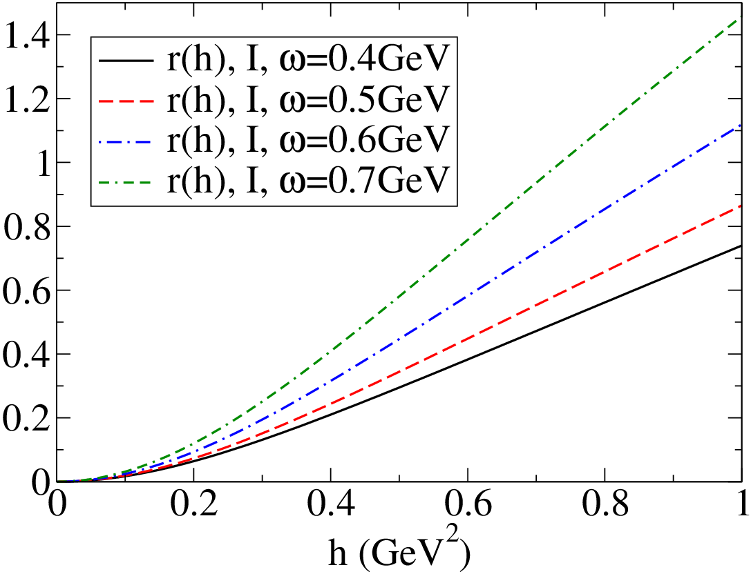

is plotted for both types of interaction and varying in Fig. 2. Recent lattice calculations, e.g., Refs. [22, 23, 24, 25, 26], indicate that for small values of () this ratio should rise quadratically with increasing and for large , linearly.22 2 We should point out that in contrast, the lattice study of Ref. [27] found that the small behavior is linear in the chiral limit, in accordance with the chiral perturbation theory result [28]. This behavior is qualitatively well-reproduced by the results here. We notice that is larger for the type I interaction and increases with the parameter . In the lattice calculation of Ref. [22], it was shown that unquenching effects are significant when considering the condensate in the presence of the magnetic field - the dynamical quark contribution was of the order of . Since the truncated gap equation studied here corresponds to a quenched system (although the parameter sets used stem from those fitted to physical observables in [19]), it makes sense to compare our results to those of Ref. [22] that only include the valence quark contributions and we choose the up-quark for concreteness (this function is labelled in Ref. [22]). To make the comparison, we have to convert the argument () with the factor for the up-quark electric charge. This is most easily done by fitting the curves for with the formula (suggested in Ref. [22])
| (76) |
The up-quark relative increment function is then given by
| (77) |
It is found that the type I interaction with (for which and ) best compares to the lattice results. The comparison is shown in Fig. 3 (the data for are extracted from Table I of Ref. [22] using the value to convert to physical units). For small , the agreement is rather striking, whereas for large , the linear rise in has a larger coefficient than for the lattice result. (Notice that in the lattice calculation of Ref. [22], the finite lattice spacing leads to saturation effects for very large magnetic fields and these tend to suppress in this region, as shown in Ref. [23].) Recalling that the approximations used to derive the quark propagator in the presence of the magnetic field, Eq. (67), were tailored to the limit, it is tempting to conclude from Fig. 3 that the type I, curve is the preferred parametrization of the model interaction. However, we urge some caution here. In this study, the chiral quark condensate is considered whereas the lattice simulation of Ref. [22] has finite bare quark masses corresponding to and it may be that the direct comparison is not appropriate without taking this into account. Additionally, the various parameter sets used in this study are chosen so as to keep the condensate (in the absence of the magnetic field) fixed, using the type I, interaction from Ref. [19] as a basis. If one were to, for example, fix the parameters via a recalculation of the meson masses and leptonic decay constants, the parameter sets may change such that a considerably more detailed analysis would be required. What is clear from Fig. 3 though, is that the small quadratic behavior and the scale of the transition between the quadratic and linear regimes is well-reproduced. It is worth pointing out that the upper estimate for the magnitude of magnetic fields in noncentral heavy-ion collisions [14] is , which coincidentally lies roughly at the transition scale between the small and large behaviors of the curves in Fig. 3.

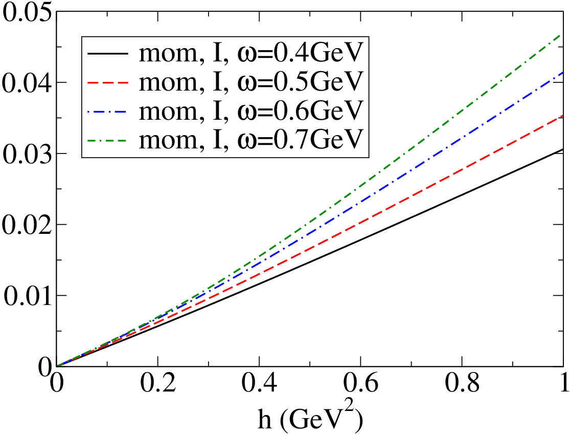

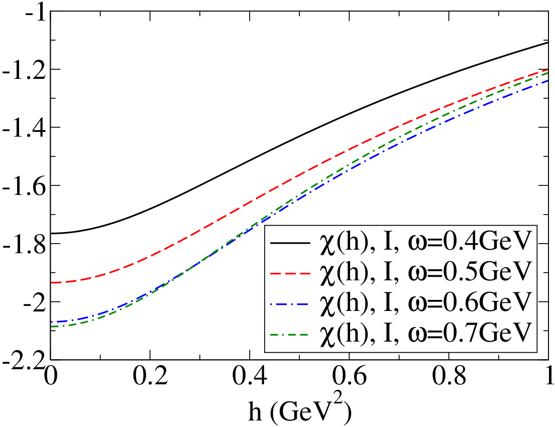
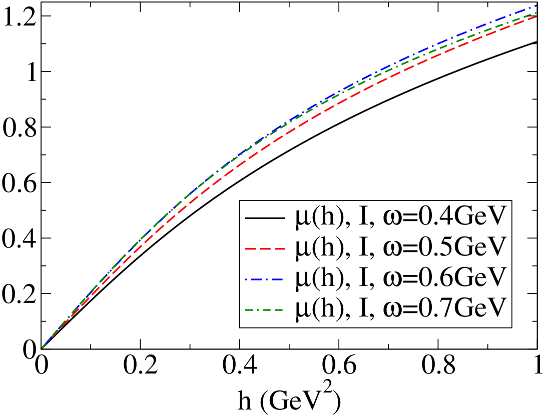
The magnetic moment, , Eq. (71), is plotted as a function of in Fig. 4. It is seen that is approximately linear for small (and vanishes for , as it should) and that it follows much the same pattern of parameter dependence as for in Fig. 2. The related function , Eq. (73), is plotted in Fig. 5. The interesting part of this plot is the limit , from which the magnetic susceptibility, , can be extracted. It is seen that approaches a constant for small values of , the lowest values calculated (numerically is the lowest nonzero value of considered) approximating and presented in Table 1. It is apparent that trying to extrapolate from with, for example, only data for , the resulting values for would be rather inaccurate because of the bend in the curves around , underscoring the need for studying the small behavior emphasized in this study. One other noticeable feature of Fig. 5 is that the type I interaction, curve appears outside the pattern of parameter dependence that one might have expected from the other curves. The explanation for this is quite straightforward. Both the magnetic moment, , plotted in Fig. 4 and the condensate, via the relative increment function, , plotted in Fig. 2 have a clear pattern of parameter dependence. However their ratio, the absolute value of which is the magnetic polarization, given by Eq. (72) and plotted in Fig. 6, shows evidence for a turning point in for increasing (at least for the type I interaction). Given that , the curve seen from this perspective no longer appears out of place.

The results for the magnetic susceptibility, , given in Table 1 can be compared with those presented in Refs. [12, 13, 25]. The (quenched, chiral limit) lattice calculation of Ref. [13] gives , the (unquenched, finite bare quark mass) lattice results presented in Ref. [25] have (for the up-quark), whereas the calculations carried out in Ref. [12] give (Nambu-Jona-Lasinio model) and (quark-meson model). Our results with lie roughly between the lattice results, but are not inconsistent with the other calculations. Related to the susceptibility, , the product is also of phenomenological interest. In Ref. [12], various estimates for this quantity were reviewed, with the numerical values . Our results, shown in Table 1 lie in the range and are somewhat smaller than this, although not dramatically so.
The magnetic polarization , defined in Eq. (72), is plotted in Fig. 6. In the lattice study of Ref. [13], it was shown that for large , there is a saturation and as . The explanation for this is based on the expected dominance of the lowest Landau level for large magnetic fields. For the lowest Landau level, the propagator is projected with (as discussed earlier) and one has the analytic result . This behavior is not reproduced here and the reason is clear – the approximations made in order to sum the Landau levels of the nonperturbative propagator were tailored to the opposite limit () and are not suitable for determining the large behavior. (Recall that this was also seen for the comparison of to the lattice data in Fig. 3.)

Interestingly though, we do see indirect evidence for the dominance of the lowest Landau level. Having performed a summation in this study, there is no direct access to the lowest Landau level contributions. However, we can look at the different spin projected dressing functions, noting that only and contribute to the lowest Landau level. Now, the dressing functions do not individually contain much direct information: for example, the dressing functions have different numerical values but the same condensate when comparing the two interaction types and various parameter sets of this study. Combinations of the dressing functions though, e.g., the condensate or the mass function, do form physically meaningful quantities which one may compare. Let us thus consider the mass function that would arise from the lowest Landau level spin structure (the self-energy terms proportional to ), the ratio evaluated at , and compare it to the ratio (associated with the component). This is plotted in Fig. 7 for both types of interaction and with . It is seen that the ratio is approximately constant with varying for both types of interaction. However, the ratio increases significantly with (dramatically so for the type I interaction). The mechanism for this is the decrease of in the infrared with increasing (see also Fig. 1). The decrease in is already present for small (where the approximations should be valid) and so by extrapolation, one would expect the -projected mass function (i.e., that connected with the spin structure of the lowest Landau level) to be dominant at large .


VI Summary and conclusions
In this paper, the quark gap equation in the presence of a constant external magnetic field was studied. The rainbow truncation was employed, with two versions of a simple phenomenological one-gluon exchange interaction. The focus was on the small magnetic field limit, motivated by three concerns: the theoretical desire to connect the results to standard results in the absence of the magnetic field, the fact that the strong interaction is typically stronger than any other interaction, and the wish to calculate the magnetic susceptibility. In order to do this, a nonperturbative approximation to the quark propagator in the presence of a small magnetic field was constructed, utilizing results [15, 16] for the summation over the Landau levels that arise when considering the Ritus eigenfunction method [10] as applied to the fermion gap equation [5, 6, 7, 8, 9].
With the phenomenological interactions considered, it was found that the chiral condensate rises quadratically for small magnetic fields and linearly for large fields, in qualitative agreement with recent lattice results [22, 23, 24, 25, 26]. Comparing to the (valence quark contribution to the) quark condensate lattice results of Ref. [22], it was seen that the position of the transition between small and large magnetic fields can be quantitatively reproduced (and gives an estimate for the range of validity of our approximation). The delineation between the small and large magnetic field behavior lies roughly at the upper estimate for the magnitudes of fields present in noncentral heavy-ion collisions [14]. The calculated magnetic susceptibility also qualitatively agreed with recent results [12, 13, 25]. It was observed that the approximated propagator does not reproduce the expected large magnetic field behavior of the magnetic polarization, although this was unsurprising given the nature of the approximations tailored to the small field limit.
At a more technical level, it was seen that the response of the system to the magnetic field was dependent on both the form of the interaction and its parametrization, despite the fact that the chiral condensate in the absence of the magnetic field was held fixed. This is in marked contrast to previous studies of the light meson mass spectrum and leptonic decay constants that employed this type of interaction [19, 21], where it was observed that the results (aside from the axialvector meson masses) were stable with respect to such parameter changes. The conclusion is that the magnetic field is a sensitive probe of the quark self-energy and the details of the interaction. From the phenomenological perspective, this might allow one to discriminate between various models and approximations.
There are several interesting applications of the approximation studied here that may be explored in future work. One may consider the generalization to finite quark masses in order to compare more directly with lattice results. Also unquenching effects, shown to be important in the lattice study of Ref. [22], might be looked at (quark loop effects were already studied in the absence of the magnetic field for this type of interaction in Ref. [29]). Further, it would be interesting to study the case of finite temperature and chemical potential to gain insight into the QCD phase diagram.
Acknowledgements.
The authors would like to thank M. D’Elia for useful correspondence, in particular concerning the comparison to lattice data. This work has been supported in part by the Deutsche Forschungsgemeinschaft (DFG) under contract no. DFG-Re856-9/1.Appendix A Hermite functions and polynomials
Let us introduce the Hermite functions, . They obey the following differential equation ()
| (78) |
and form an orthonormal and complete set:
| (79) |
The following recursion relations prove invaluable:
| (80) |
It is useful to define explicitly. The Hermite functions are related to the more usual Hermite polynomials, , (and parabolic cylinder functions) by
| (81) |
The generating function for the Hermite functions is given via the identity
| (82) |
Because of the Gaussian nature of the generating function, the Fourier transform of the Hermite polynomials may be performed and
| (83) |
Notice the following identity [30]:
| (84) |
where is a Laguerre polynomial ( and ). Further,
| (85) |
Appendix B Explicit form of the gap equation
For completeness, we present the explicit form for the gap equation used in numerical work. The expressions are derived as follows. The nonperturbative decompositions for the proper two-point function , Eq. (59), and the propagator , Eq. (67), both have the form presented in Eq. (34) and are inserted into the gap equation, Eq. (35), along with either of the interaction forms, Eq. (33). The Schwinger phase is simply an overall factor. The various Dirac components are then projected to generate a set of scalar equations. Finally, a Wick rotation to Euclidean space is performed. In the presence of the magnetic field, the dressing functions - are functions of two variables, and (in Euclidean space, ). The explicit equations for a chiral quark () then read ()
| (86) |
In the above,
| (87) |
is the factor that distinguishes between the two types of interaction. The propagator denominator factor occurring in the integrals above is given by
| (88) |
where all dressing functions are evaluated with the argument . The various combinations of propagator numerator factors (with the same arguments as for ) are
| (89) |
Finally, the integration kernels read
| (90) |
References
- [1] I. A. Shovkovy, Lect. Notes Phys. 871, 13 (2013) [arXiv:1207.5081 [hep-ph]].
- [2] V. P. Gusynin, V. A. Miransky and I. A. Shovkovy, Phys. Rev. Lett. 73, 3499 (1994) [Erratum-ibid. 76, 1005 (1996)] [hep-ph/9405262].
- [3] V. P. Gusynin, V. A. Miransky and I. A. Shovkovy, Phys. Lett. B 349, 477 (1995) [hep-ph/9412257].
- [4] V. P. Gusynin, V. A. Miransky and I. A. Shovkovy, Phys. Rev. D 52, 4747 (1995) [hep-ph/9501304].
- [5] C. N. Leung, Y. J. Ng and A. W. Ackley, Phys. Rev. D 54, 4181 (1996) [hep-th/9512114].
- [6] D. S. Lee, C. N. Leung and Y. J. Ng, Phys. Rev. D 55, 6504 (1997) [hep-th/9701172].
- [7] C. N. Leung and S. -Y. Wang, Annals Phys. 322, 701 (2007) [hep-ph/0503298].
- [8] A. Ayala, A. Bashir, A. Raya and E. Rojas, Phys. Rev. D 73, 105009 (2006) [hep-ph/0602209].
- [9] E. Rojas, A. Ayala, A. Bashir and A. Raya, Phys. Rev. D 77, 093004 (2008) [arXiv:0803.4173 [hep-ph]].
- [10] V. I. Ritus, Sov. Phys. JETP 48, 788 (1978) [Zh. Eksp. Teor. Fiz. 75, 1560 (1978)].
- [11] V. I. Ritus in Issues in Intense-Field Quantum Electrodynamics, ed. V. L. Ginzburg (Nova Science, Commack, 1987).
- [12] M. Frasca and M. Ruggieri, Phys. Rev. D 83, 094024 (2011) [arXiv:1103.1194 [hep-ph]].
- [13] P. V. Buividovich, M. N. Chernodub, E. V. Luschevskaya and M. I. Polikarpov, Nucl. Phys. B 826, 313 (2010) [arXiv:0906.0488 [hep-lat]].
- [14] V. Skokov, A. Y. .Illarionov and V. Toneev, Int. J. Mod. Phys. A 24, 5925 (2009) [arXiv:0907.1396 [nucl-th]].
- [15] E. V. Gorbar, V. A. Miransky, I. A. Shovkovy and X. Wang, Phys. Rev. D 88, 025025 (2013) [arXiv:1304.4606 [hep-ph]].
- [16] E. V. Gorbar, V. A. Miransky, I. A. Shovkovy and X. Wang, Phys. Rev. D 88, 025043 (2013) [arXiv:1306.3245 [hep-ph]].
- [17] C. Itzykson and J. B. Zuber, “Quantum Field Theory,” New York, Usa: Mcgraw-hill (1980) 705 P.(International Series In Pure and Applied Physics).
- [18] A. Chodos, K. Everding and D. A. Owen, Phys. Rev. D 42, 2881 (1990).
- [19] R. Alkofer, P. Watson and H. Weigel, Phys. Rev. D 65, 094026 (2002) [hep-ph/0202053].
- [20] A. C. Aguilar and J. Papavassiliou, Phys. Rev. D 83, 014013 (2011) [arXiv:1010.5815 [hep-ph]].
- [21] P. Maris and P. C. Tandy, Phys. Rev. C 60, 055214 (1999) [nucl-th/9905056].
- [22] M. D’Elia and F. Negro, Phys. Rev. D 83, 114028 (2011) [arXiv:1103.2080 [hep-lat]].
- [23] M. D’Elia, J. Phys. Conf. Ser. 432, 012004 (2013).
- [24] G. S. Bali, F. Bruckmann, G. Endrodi, Z. Fodor, S. D. Katz and A. Schafer, Phys. Rev. D 86, 071502 (2012) [arXiv:1206.4205 [hep-lat]].
- [25] G. S. Bali, F. Bruckmann, M. Constantinou, M. Costa, G. Endrödi, Z. Fodor, S. D. Katz and S. Krieg et al., PoS ConfinementX , 198 (2012) [arXiv:1301.5826 [hep-lat]].
- [26] P. V. Buividovich, M. N. Chernodub, E. V. Luschevskaya and M. I. Polikarpov, Phys. Lett. B 682, 484 (2010) [arXiv:0812.1740 [hep-lat]].
- [27] E. -M. Ilgenfritz, M. Kalinowski, M. Muller-Preussker, B. Petersson and A. Schreiber, Phys. Rev. D 85, 114504 (2012) [arXiv:1203.3360 [hep-lat]].
- [28] I. A. Shushpanov and A. V. Smilga, Phys. Lett. B 402, 351 (1997) [hep-ph/9703201].
- [29] C. S. Fischer, P. Watson and W. Cassing, Phys. Rev. D 72, 094025 (2005) [hep-ph/0509213].
- [30] I. S. Gradshteyn and I. M. Ryzhik, Table of Integrals, Series and Products (5th edition, Academic Press, 1994).