A Tractable State-Space Model for Symmetric Positive-Definite Matrices

A state-space model is often characterized by an observation density $f(y_{t}|x_{t})$ for the responses $\{y_{t}\}_{t=1}^{T}$ and a transition density $g(x_{t}|x_{t-1})$ for the latent states $\{x_{t}\}_{t=1}^{T}$. Usually, the latent states can take on any value in $\mathbb{R}^{n}$; however, there are times when the states or the responses are constrained to a manifold embedded in $\mathbb{R}^{n}$. For instance, econometricians and statisticians have devised symmetric positive-definite matrix-valued statistics that can be interpreted as noisy observations of the conditional covariance matrix of a vector of daily asset returns. In that case, it is reasonable to consider a state-space model that has covariance matrix-valued responses (the statistics) and covariance matrix-valued latent quantities (the time-varying covariance matrices).

Unfortunately, devising state-space models on curved spaces (like the set of covariance matrices) that lend themselves to Bayesian analysis is not easy. Just writing down the observation and transition densities can be difficult in this setting, since one must define distributions on curved spaces. Asking that these densities then lead to some recognizable posterior distribution for the latent states and the system’s parameters compounds the problem. Filtering is slightly less daunting, since one can appeal to sequential methods. (Filtering or forward filtering refers to iteratively deriving the filtered distributions $p(x_{t}|\mathcal{D}_{t},\theta)$ where $\mathcal{D}_{t}$ is the data $\{y_{s}\}_{s=1}^{t}$ and $\theta$ represents the system’s parameters.) Approximate methods can also flounder. For instance, when $y_{t}$ and $x_{t}$ exist in planar spaces, it is common to write down observation and evolution equations and only specify the first and second moments of the evolution innovations and observation errors, which leads to tractable methods for filtering. However, the notions of mean and variance do not translate automatically to curved spaces and hence even this density-less approach runs into trouble.

Despite these difficulties, it is still of interest to develop state-space models for the set of covariance matrices and other curved spaces, since such data exists. In addition to the financial application described previously, time-varying covariance matrices arise in computer vision (Porikli et al., 2006), and time varying linear subspaces arise in subspace tracking (Srivastava and Klassen, 2004). Some work has explored forward filtering such data. Tyagi and Davis (2008) develop a Kalman-like filter (Kalman, 1960) for symmetric positive-definite matrices while Hauberg et al. (2013) develop an algorithm similar to the unscented Kalman filter (Julier and Uhlmann, 1997) for geodesically complete manifolds. Several collaborations have made use of particle filters: Srivastava and Klassen (2004) for the Grassmann manifold, Tompkins and Wolfe (2007) for the Steifel manifold, Kwon and Park (2010) for the affine group, and Choi and Christensen (2011) for the special Euclidean group.

None of these approaches have produced a state-space model amenable to fully Bayesian inference—inference in which one can compute both the conditional and marginalized versions of the filtered, smoothed, and predictive distributions (where the conditioning and marginalizing is with respect to $\theta$) in addition to the joint posterior distribution of the latent states and the system’s parameters. (Smoothing refers to computing the distribution of past states while predicting refers to computing the distribution of future states.) One attempt in that direction, Prado and West (2010) (p. 273), partially address these issues for dynamic covariance matrices, but informally and with less flexibility than the forthcoming.

We fully address these issues for a state-space model with symmetric positive-definite or positive semi-definite rank-$k$ observations and symmetric positive-definite latent states. (Let $\mathcal{S}_{m,k}^{+}$ denote the set of order $m$, rank $k$, symmetric positive semi-definite matrices and let $\mathcal{S}_{m}^{+}$ denote the set of order $m$, symmetric positive-definite matrices.) The model builds on the work of Uhlig (1997), who showed how to construct a state-space model with $\mathcal{S}_{m,1}^{+}$ observations and $\mathcal{S}_{m}^{+}$ hidden states and how, using this model, one can forward filter in closed form. We extend his approach to observations of arbitrary rank and show how to forward filter, how to backward sample, and how to marginalize the hidden states to estimate the system’s parameters, all without appealing to fanciful MCMC schemes. (Backward sampling refers to taking a joint sample of the posterior distribution of the latent states $p(\{x_{t}\}_{t=1}^{T}|\mathcal{D}_{T},\theta)$ using the conditional distributions $p(x_{t}|x_{t+1},\mathcal{D}_{t},\theta)$.) The model’s estimates and one-step ahead predictions are exponentially weighted moving averages (also known as geometrically weighted moving averages). Exponentially weighted moving averages are known to provide simple and robust estimates and forecasts in many settings (Brown, 1959).

The model herein is closely related to several models found in the Bayesian literature, all of which have their origin in variance discounting techniques (Quintana and West, 1987; West and Harrison, 1997). Uhlig (1997) provided a rigorous justification for variance discounting, showing that it is a form of Bayesian filtering for covariance matrices, and our model can be seen as a direct extension of Uhlig’s work. (Shephard (1994) constructs a similar model, but only for the univariate case.) The model of Prado and West (2010) (p. 273) is similar to ours, though less flexible.

Uhlig (1997) considers observations, $\mathbf{r}_{t}\in\mathbb{R}^{m}$, $t=1,\ldots,T$, that are conditionally normal given the hidden states $\{\mathbf{X}_{t}\}_{t=1}^{T}$, which take values in $\mathcal{S}^{+}_{m}$. We will henceforth write vectors in bold lower case and matrices in bold upper case. In particular, assuming $\mathbb{E}[\mathbf{r}_{t}]=0$, his model is

where $n>m-1$ is an integer and $\beta_{m}$ is the multivariate beta distribution, which is defined in Section 5. This model possesses closed form formulas for forward filtering that only requires knowing the outer product $\mathbf{r}_{t}\mathbf{r}_{t}^{\prime}$; thus, one may arrive at equivalent estimates of the latent states by letting $\mathbf{Y}_{t}=\mathbf{r}_{t}\mathbf{r}_{t}^{\prime}$ and using the observation distribution

where $W_{m}(1,\mathbf{X}_{t}^{-1})$ is the order $m$ Wishart distribution with $1$ degree of freedom and scale matrix $\mathbf{X}_{t}^{-1}$ as defined in Section 5. We show that one can extend this model for $\mathbf{Y}_{t}$ of any rank:

where $n>m-1$ and $k$ is an integer less than $m$ or is a real number greater than $m-1$. (When $k$ is an integer less than $m$, $\mathbf{Y}_{t}$ has rank $k$.) Many of the mathematical ideas needed to motivate Model UE (for Uhlig extension) can be found in a sister paper (Uhlig, 1994) to the Uhlig (1997) paper, and Uhlig could have written down the above model given those results; though, he was focused specifically on the rank-deficient case, and the rank-1 case in particular, as his 1997 work shows. We contribute to this discourse by constructing the model in a fashion that makes sense for observations of all ranks, show that one may backward sample to generate a joint draw of the hidden states, and demonstrate that one may marginalize the hidden states to estimate the system’s parameters $n$, $k$, and $\lambda$.

Model UE has a slightly different form and significantly more flexibility than the model of Prado and West (2010) (see p. 273), which is essentially

As noted by Prado and West, $\lambda$ is constrained “to maintain a valid model, since we require either $h_{t}>m-1$ or $h_{t}$ be integral [and less than $m$]. The former constraint implies that $\lambda$ cannot be too small, $\lambda>(m-2)/(m-1)$ defined by the limiting value.” If $h_{t}=h$ is integral, then $\lambda=(h-1)/h$. Thus, one cannot pick from a range of $\lambda$ for $h\leq m-1$, when $h$ must be an integer, which means there are only $m-2$ allowed values of $\lambda$ for $\lambda\leq(m-2)/(m-1)$, the limiting value when $h_{t}$ is sufficiently large. When $m$ is large this is a severe restriction. Further, for $m\geq 2$, $h=2$ produces the smallest possible value of $\lambda$; thus, $\lambda$ cannot be below $1/2$ unless $m=1$. (We have replaced Prado and West’s $\beta$ by $\lambda$ and their $q$ by $m$.) The parameter $\lambda$ is important since it controls how much the model smooths observations when forming estimates and one-step ahead predictions; thus the constraints on $\lambda$ are highly undesirable. In contrast, our model lets $\lambda$ take on any value.

Given Model UE, we can derive several useful propositions. The proofs of these propositions, which synthesize and add to results from Uhlig (1994), Muirhead (1982) Díaz-García and Jáimez (1997), are technical, and hence we defer their presentation to Section 5. Presently, we focus on the closed form formulas that one may make use of when forward filtering, backward sampling, predicting one step into the future, and estimating $n$, $k$, and $\lambda$.

First, some notation: inductively define the collection of data $\mathcal{D}_{t}=\{\mathbf{Y}_{t}\}\cup\mathcal{D}_{t-1}$ for $t=1,\ldots,T$ with $\mathcal{D}_{0}=\{\mathbf{\Sigma}_{0}\}$ where $\mathbf{\Sigma}_{0}$ is some covariance matrix. Let the prior for $(\mathbf{X}_{1}|\mathcal{D}_{0})$ be $W_{m}(n,(k\mathbf{\Sigma}_{0})^{-1}/\lambda)$ where $W_{m}(d,\mathbf{V})$ is the Wishart distribution with $d\in\{1,\ldots,m-1\}\cap(m-1,\infty)$ degrees of freedom and scale matrix $\mathbf{V}$. (See Definition 4 for details.) In the following, we implicitly condition on the parameters $n$, $k$, and $\lambda$.

Examining the one-step ahead forecasts of $\mathbf{Y}_{t}$ elucidates how the model smooths. Invoking the law of iterated expectations, one finds that $\mathbb{E}[\mathbf{Y}_{t+1}|\mathcal{D}_{t}]=\mathbb{E}[\mathbf{X}_{t+1}^{-1}|\mathcal{D}_{t}]$. Since $(\mathbf{X}_{t+1}^{-1}|\mathcal{D}_{t})$ is an inverse Wishart distribution, its expectation is proportional to $\mathbf{\Sigma}_{t}$. Solving the recursion for $\mathbf{\Sigma}_{t}$ from Fact 1 shows that

Thus, the forecast of $\mathbf{Y}_{t+1}$ will be a scaled, geometrically weighted average of the previous observations. If, further, one enforces the constraint

then taking a step from $\mathbf{X}_{t}$ to $\mathbf{X}_{t+1}$ does not change its harmonic average, that is $\mathbb{E}[\mathbf{X}_{t}^{-1}|\mathcal{D}_{t}]=\mathbb{E}[\mathbf{X}_{t+1}^{-1}|\mathcal{D}_{t}]$. It also implies that the one-step ahead point forecast of $(\mathbf{Y}_{t+1}|\mathcal{D}_{t})$ is

Hence in the constrained case, the one-step ahead forecast is the geometrically weighted average of past observations. For a geometrically weighted average, the most recent observations are given more weight as $\lambda$ decreases. It has been known for some time that such averages provide decent one-step ahead forecasts (Brown, 1959).

As noted initially, Model UE is an extension of the one proposed by Uhlig (1997). For the original model, when $k=1$, one might consider observing a vector of heteroskedastic asset returns $\mathbf{r}_{t}\sim N(0,\mathbf{X}_{t}^{-1})$ where the precision matrix $\mathbf{X}_{t}$ changes at each time step. The extended model allows the precision matrix to change less often than the frequency with which the returns are observed. For instance, one may be interested in estimating the variance of the daily returns, assuming that the variance only changes from day to day, using multiple observations taken from within the day.

To that end, suppose the vector of intraday stock prices evolves as geometric Brownian motion so that on day $t$ the $m$-vector of log prices is

at time $s$, where $s$ the fraction of the trading day that has elapsed, $\{\mathbf{w}_{s}\}_{s\geq 0}$ is an $m$-dimensional Brownian motion, and $\mathbf{V}_{t}^{1/2}{\mathbf{V}_{t}^{1/2}}^{\prime}=\mathbf{X}^{-1}_{t}$. In practice, $\mathbf{\mu}$ is essentially zero, so we will ignore that term. Further, suppose one has viewed the vector of prices at $k+1$ equispaced times throughout the day so that $\mathbf{r}_{t,i}=\mathbf{p}_{t,i}-\mathbf{p}_{t,i-1/k},\;i=1/k,\ldots,1.$ Then $\mathbf{r}_{t,i}\sim N(0,\mathbf{X}_{t}^{-1}/k)$ and $\mathbf{Y}_{t}=\sum_{i=1}^{k}\mathbf{r}_{t,i}\mathbf{r}_{t,i}^{\prime}$ is distributed as $W_{m}(k,\mathbf{X}_{t}^{-1}/k)$. Letting $\mathbf{X}_{t}=\mathcal{U}(\mathbf{X}_{t-1})^{\prime}\mathbf{\Psi}_{t}\mathcal{U}(\mathbf{X}_{t-1})$ where $\mathcal{U}(\cdot)$ computes the upper Cholesky decomposition and $\mathbf{\Psi}_{t}\sim\beta_{m}(n/2,k/2)$, we recover Model UE exactly. Of course, in reality, returns are not normally distributed; they are heavy tailed and there are diurnal patterns within the day. Nonetheless, the realized covariance literature, which we discuss in more detail in Section A, suggests that taking $\mathbf{Y}_{t}$ to be an estimate of the daily variance $\mathbf{X}_{t}^{-1}$ is a reasonable thing to do; though to suppose that the error is Wishart is a strong assumption. More dubious is the choice of the evolution equation for $\mathbf{X}_{t}$; a point we discuss further in Section 4. But the evolution equation for $\{\mathbf{X}_{t}\}_{t=1}^{T}$ does provide a likelihood that accommodates closed form forward filtering and backward sampling formulas, and possesses only a few parameters, which makes it a relatively cheap model to employ.

The one mild challenge when applying the model is estimating $\mathbf{\Sigma}_{0}$. However, it is possible to “cheat” and not actually estimate $\mathbf{\Sigma}_{0}$ at all. Consider (1) and ponder the following two observations. First, $\mathbf{\Sigma}_{t}$ is a geometrically weighted sum in $\{\mathbf{\Sigma}_{0},\mathbf{Y}_{1},\ldots,\mathbf{Y}_{t}\}$. Second, the least important term in the sum is $\mathbf{\Sigma}_{0}$. Thus, one can reasonably ignore $\mathbf{\Sigma}_{0}$ if $t$ is large enough. To that end, we suggest setting aside the first $\tau_{1}$ observations and using $\{\mathbf{\Sigma}_{\tau_{1}},\mathbf{Y}_{\tau_{1}+1},\ldots,\mathbf{Y}_{\tau_{2}}\}$ where $\mathbf{\Sigma}_{\tau_{1}}=\sum_{i=0}^{\tau_{1}}\lambda^{i}\mathbf{Y}_{\tau_{1}-i}$ to learn $n$, $k$, and $\lambda$ using Proposition 3 and the prior $p(X_{\tau_{1}+1}|\mathcal{D}_{\tau_{1}})\sim W_{m}(n,(k\Sigma_{\tau_{1}})^{-1}/\lambda)$. It may seem costly to disregard the first $\tau_{1}$ observations, but since there are so few parameters to estimate this is unlikely to be a problem—the remaining data will suffice.

This is the process used to generate Figure 1 (with $\tau_{1}=50$ and $\tau_{2}=100$). The data set follows the $m=30$ stocks that comprised the Dow Jones Industrial Average in October, 2010. Eleven intraday observations were taken every trading day for almost four years to produce 927 daily, rank-10 observations $\{\mathbf{Y}_{t}\}_{t=1}^{927}$. Since the observations are rank-deficient, we know that $k=10$. (In the full-rank case, we will estimate $k$.) We constrain $\lambda$ using (2) so that the only unknown is $n$. Given an improper flat prior for $n>29$, the posterior mode is $n=190$, implying that $\lambda=0.94$, a not unusual value for exponential smoothing. Once $n$ is set, one can filter forward, backward sample, and generate one-step ahead predictions in closed form. The right side of Figure 1 shows the filtered covariance between Alcoa Aluminum and American Express on the correlation scale.

However, one need not take such a literal interpretation of the model. Instead of trying to justify its use on first principles, one may simply treat it as a covariance-valued state-space model, which we do presently. As noted in the introduction and elaborated on in Section A, realized covariance matrices are good estimates of the daily covariance matrix of a vector of financial asset returns. Since realized covariance matrices are good estimates it is natural to try to use them for prediction. The statistics themselves place very few restrictions on the distribution of asset prices and their construction is non-parametric. In other words, the construction of a realized covariance matrix (at least the construction we use) says little about the evolution of the latent daily covariance matrices.

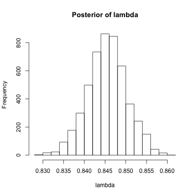
But we do not need to know the exact evolution of the latent daily covariance matrices to employ Model UE to make short-term predictions. To that end, we may treat realized covariance matrices $\{\mathbf{Y}_{t}\}_{t=1}^{T}$ as $\mathcal{S}_{m}^{+}$-valued data that track the latent daily covariances $\{\mathbf{X}_{t}^{-1}\}_{t=1}^{T}$. We construct these realized statistics using the same $m=30$ stocks over the same time period as above, but using all of the intraday data, which results in full-rank observations (see Section B for details). We follow the same basic procedure as above to estimate $k$ and $n$, and implicitly $\lambda$ by constraint (2). Selecting an improper flat prior for $n>29$ and $k>29$ yields the log-posterior found in Figure 2. The posterior mode is at $(67,396)$ implying $\lambda=0.85$. The gray lines in Figure 2 correspond level sets of $\lambda$ in $k$ and $n$. As seen in the figure, the uncertainty in $(k,n)$ is primarily in the direction of the steepest ascent of $\lambda$. One can use Proposition 3 and the method of generating $\Sigma_{\tau_{1}}$ to construct a random walk Metropolis sampler as well. Doing that we find the posterior mean to be $(67,399)$, which implies an essentially identical $\lambda$. A histogram of the posterior of $\lambda$ is in Figure 3, showing that, though the the direction of greatest variation in $(k,n)$ corresponds to changes in $\lambda$, the subsequent posterior standard deviation of $\lambda$ is small.

Recall, our original motivation for studying $\mathcal{S}_{m}^{+}$-valued state-space models was the observation that exponentially smoothing realized covariance matrices generates better one-step ahead predictions than factor stochastic volatility. In those initial experiments, we used cross-validation to pick the smoothing parameter $\lambda$. Figure 3 shows that one arrives at the same conclusion under two different measures of performance using Model UE and the method described previously to pick $\lambda$. The mesures are described in the caption to Figure 3. To summarize: it is better to use our simple $\mathcal{S}_{m}^{+}$-valued state-space model with realized covariance matrices to make short term predictions than it is to use factor stochastic volatility with only daily returns.

Though we pick a point estimate of the system’s parameters above and then fix that value to make predictions, one can operate in a fully Bayesian manner when computing one-step ahead predictions as well as filtered distributions and the posterior distribution of the latent states. In particular, one can sample the posterior distribution $p(\theta|\mathcal{D}_{t})$, $\theta=(k,n)$, and then use those posterior samples to draw from $p(\mathbf{X}_{t}|\mathcal{D}_{t},\theta)$ or $p(\mathbf{X}_{t+1}|\mathcal{D}_{t},\theta)$ using forward filtering or to draw from $p(\{\mathbf{X}_{s}\}_{s=1}^{t}|\mathcal{D}_{t},\theta)$ using forward filtering and backward sampling to get the corresponding joint distributions $p(\mathbf{X}_{t},\theta|\mathcal{D}_{t})$, $p(\mathbf{X}_{t+1},\theta|\mathcal{D}_{t})$, and $p(\{\mathbf{X}_{s}\}_{s=1}^{t},\theta|\mathcal{D}_{t})$.

Employing exponentially weighted moving averages to generate short-term forecasts is not new. These methods were popular at least as far back as the first half of the 20th century (Brown, 1959). In light of this, it may seem that Model UE is rather unglamorous. But this is only because we have explicitly identified how the model uses past observations to make predictions. In fact, many models of time-varying variance behave similarly. For instance, GARCH (Bollerslev, 1986) does exponential smoothing with mean reversion to predict the variance using square returns. Stochastic volatility (Taylor, 1982) does exponential smoothing with mean reversion to predict the log variance using log square returns. Models that include a leverage effect do exponential smoothing so that the amount of smoothing depends on the direction of the returns. Thus, it should not be surprising or uninteresting when a state-space model generates predictions with exponential smoothing or some variation thereof.

This helps explains why a simple model (UE) with high-quality observations can generate better short-term predictions than a complicated model (factor stochastic volatility) with low-quality data. First, both models, in one way or another, are doing something similar to exponential smoothing. Second, the true covariance process seems to revert quite slowly. Thus, there will not be much difference between a one-step ahead forecast that lacks mean reversion (Model UE) and a one-step ahead forecast that includes mean reversion (factor stochastic volatility). Since the prediction mechanisms are similar, the model that uses a “higher resolution” snapshot of the latent covariance matrices has the advantage. Of course, these observations only apply when using factor stochastic volatility with daily returns. It may be the case that one can use intraday information along with some specialized knowledge about the structure of market fluctuations (like factor stochastic volatility) to generate better estimates and predictions.

Despite Model UE’s short-term forecasting success, it does have some faults. First, the evolution of $\{\mathbf{X}_{t}\}_{t=1}^{T}$ can be rather degenerate. In the one-dimensional case, when $\{\log x_{t}\}_{t=1}^{\infty}$ is not a martingale, $\{x_{t}\}_{t=1}^{\infty}$ either almost surely converges to zero or almost surely diverges. (The discussion before Proposition 8 expands upon this point.) Presumably, the multivariate case suffers from something similar and, clearly, this does not reflect the dynamics we want to capture. Second, its $k$-step ahead predictions do not revert to some mean, which is what one would expect when modeling a stationary process. In fact, the first point suggests that things are worse than that: the $k$-step ahead predictive distributions may degenerate. Consequently, the model will perform poorly as the horizon of the prediction increases.

Thus, to the larger question, “How does one construct rich, tractable state-space models on curved spaces,” we only gave a partial answer, showing how to create a tractable model—one in which the densities of interest may be computed and sampled. In essence, descriptive richness was sacrificed for tractability. One might proceed in the opposite direction by endowing the latent process with rich dynamics initially. For instance, one may transform a positive-definite matrix $\mathbf{X}$ into an unconstrained planar coordinate system using the factorization $\mathbf{U}^{\prime}\exp(\mathbf{D})\mathbf{U}=\mathbf{X}$, where $\mathbf{U}$ is upper triangular, $\mathbf{D}$ is diagonal, and $\exp$ is the matrix exponential, and then model the dynamics in the planar coordinates $(\mathbf{U},\mathbf{D})$. But, in that case, one must deal with a potentially inconvenient distribution in the $\mathbf{X}$ coordinates for forward filtering or backward sampling. Comparing the benefits of each approach within the context of Bayesian state-space inference is left to future work.

Much of the calculus one needs can be found Uhlig (1994) or Muirhead (1982). We synthesize those results here. We are not aware of results in either regarding backward sampling or marginalization.

First, some notation: Assume $k,m\in\mathbb{N}$, $k\leq m$. Let $\mathcal{S}^{+}_{m,k}$ denote the set of positive semi-definite symmetric matrices of rank $k$ and order $m$. When $k=m$, we drop $k$ from the notation so that $\mathcal{S}^{+}_{m}$ denotes the set of positive-definite symmetric matrices of order $m$. For symmetric matrices $\mathbf{A}$ and $\mathbf{B}$, let $\mathbf{A}<\mathbf{B}$ denote $\mathbf{B}-\mathbf{A}\in\mathcal{S}_{m}^{+}$ . For $\mathbf{A}\in\mathcal{S}^{+}_{m}$ let

If $k>m-1$ is real and we write $\mathcal{S}_{m,k}^{+}$ then we implicitly mean $\mathcal{S}_{m}^{+}$. We will use $|\cdot|$ to denote the determinant of a matrix and $\mathbf{I}$ to denote the identity. We at times follow Muirhead (1982) and define densities with respect to differential forms (also known as $K$-forms or differential $K$-forms). Mikusiński and Taylor (2002) is a good introduction to calculus on manifolds. The handouts of Edelman (2005) provide a more succinct introduction.

The following theorem synthesizes results from Uhlig (1994), Muirhead (1982), and Díaz-García and Jáimez (1997).

Theorem 7 justifies forward filtering in Model UE as follows.

The reader may notice that the choice of distribution for $\mathbf{\Psi}_{t}$ is precisely the one that facilitates forward filtering. In particular, assuming that $(\mathbf{X}_{t-1}|\mathcal{D}_{t-1})$ has an acceptable distribution to start, then $(\mathbf{X}_{t}|\mathcal{D}_{t-1})$ will have an acceptable distribution to update, so that $(\mathbf{X}_{t}|\mathcal{D}_{t})$ will have a distribution that lets us play the game all over again. However, we cannot easily write down the distribution of $(\mathbf{X}_{t+k}|\mathcal{D}_{t})$ for anything but $k=0$ or $1$. To see why, assume that we start at time $t-1$ with data $\mathcal{D}_{t-1}$ and evolve to $(\mathbf{X}_{t}|\mathcal{D}_{t-1})\sim W_{m}(n,(k\mathbf{\Sigma}_{t-1})^{-1}/\lambda)$ just like above. Now consider moving from $\mathbf{X}_{t}$ to $\mathbf{X}_{t+1}$ without updating:

The distribution of $\mathbf{I}-\mathbf{\Psi}_{t}$ is $\beta_{m}(n/2,k/2)$ but the distribution of $(\mathbf{X}_{t}|\mathcal{D}_{t-1})$ is $W_{m}(n,\ldots)$. We cannot apply Theorem 7 at this point because there is a mismatch in the degrees of freedom of $(\mathbf{X}_{t}|\mathcal{D}_{t-1})$ and the parameters of $\mathbf{I}-\mathbf{\Psi}_{t}$—we need $n+k$ not $n$ degrees of freedom! Thus, the distribution of $(\mathbf{X}_{t+1}|\mathcal{D}_{t-1})$ is unknown.

Despite not knowing its distribution, one can show that the evolution of $\{\mathbf{X}_{t}\}_{t=1}^{T}$ is rather degenerate. To see this, consider the one dimensional case, in which

Following Shephard (1994), transforming this equation by the logarithm yields

where $w_{t}=\log x_{t}$ and $\nu_{t}=\log(\psi_{t}/\lambda)$. Let $m=\mathbb{E}[\nu_{t}]$. When $m\neq 0$, the law of large numbers says that for almost every path there is some $t^{*}$ such that $t(m-|m|/2)<w_{t}<t(m+|m|/2)$ for $t>t^{*}$. That is, the paths diverge. Hence, when $m\neq 0$, the paths of $x_{t}$ either converge to $0$ or diverge. The same phenomenon can be seen when numerically simulating data in the multivariate case. This makes generating synthetic data difficult since $\mathbf{X}_{t}$ can quickly become numerically singular. It also implies that the predictive distributions are unruly.

References

- Aguilar and West [2000] O. Aguilar and M. West. Bayesian dynamic factor models and portfolio allocation. Journal of Business and Economic Statistics, 18(3):338–357, July 2000.
- Andersen et al. [2001] T. G. Andersen, T. Bollerslev, F. X. Diebold, and H. Ebens. The distribution of realized stock return volatility. Journal of Financial Econometrics, 61:43–76, 2001.
- Barndorff-Nielsen and Shephard [2002] O. E. Barndorff-Nielsen and N. Shephard. Econometric analysis of realized volatility and its use in estimating stochastic volatility. Journal of the Royal Statistical Society: Series B (Statistical Methodology), 64(2):253–280, 2002.
- Barndorff-Nielsen et al. [2009] O. E. Barndorff-Nielsen, P. R. Hansen, A. Lunde, and N. Shephard. Realized kernels in practice: Trades and quotes. Econometrics Journal, 12(3):C1–C32, 2009.
- Barndorff-Nielsen et al. [2011] O. E. Barndorff-Nielsen, P. R. Hansen, A. Lunde, and N. Shephard. Multivariate realized kernels: Consistent positive semi-definite estimators of the covariation of equity prices with noise and non-synchronous trading. Journal of Econometrics, 162:149–169, 2011.
- Bollerslev [1986] T. Bollerslev. Generalized autoregressive conditional heteroskedasticity. Journal of Econometrics, 31:307–327, 1986.
- Brown [1959] R. G. Brown. Statistical Forecasting for Inventory Control. McGraw-Hill, 1959.
- Choi and Christensen [2011] C. Choi and H. I. Christensen. Robust 3d visual tracking using particle filters on the SE(3) group. In IEEE International Conference on Robotics and Automation, pages 4384–4390, 2011.
- Díaz-García and Jáimez [1997] J. A. Díaz-García and R. G. Jáimez. Proof of the conjectures of H. Uhlig on the singular multivariate beta and the Jacobian of a certain matrix transformation. The Annals of Statistics, 25:2018–2023, 1997.
- Edelman [2005] A. Edelman. The mathematics and applications of (finite) random matrices, 2005. URL http://web.mit.edu/18.325/www/handouts.html. See handouts 1-4.
- Hauberg et al. [2013] S. Hauberg, F. Lauze, and K. S. Pedersen. Unscented Kalman filtering on Riemannian manifolds. J Math Imaging Vis, 46:103–120, 2013.
- Jacod and Shiryaev [2003] J. Jacod and A. N. Shiryaev. Limit Theorems For Stochastic Processes. Springer, 2003.
- Julier and Uhlmann [1997] S. J. Julier and J. K. Uhlmann. New extensions of the Kalman filter to nonlinear systems. In Signal Processing, Sensor Fusion, and Target Recognition VI, volume 3068, 1997.
- Kalman [1960] R. E. Kalman. A new approach to linear filtering and prediction problems. Journal of Basic Engineering, 82 (Series D):35–45, 1960.
- Karatzas and Shreve [1991] I. Karatzas and S. E. Shreve. Brownian Motion and Stochastic Calculus. Springer, 1991.
- Koopman et al. [2005] S. J. Koopman, B. Jungbackera, and E. Hol. Forecasting daily variability of the S&P 100 stock index using historical, realised and implied volatility measurements. Journal of Empirical Finance, 12:445–475, 2005.
- Kwon and Park [2010] J. Kwon and F. C. Park. Visual tracking via particle filtering on the affine group. The International Journal of Robotics Research, 29:198–217, 2010.
- Liu [2009] Q. Liu. On portfolio optimization: How and when do we benefit from high-frequency data? Journal of Applied Econometrics, 24:560–582, 2009.
- Mikusiński and Taylor [2002] P. Mikusiński and M. D. Taylor. An Introduction to Multivariate Analysis. Birkhäuser, 2002.
- Muirhead [1982] R. J. Muirhead. Aspects of Multivariate Statistical Theory. Wiley, 1982.
- Porikli et al. [2006] F. Porikli, O. Tuzel, and P. Meer. Covariance tracking using model update based on Lie algebra. In Computer Vision and Pattern Recognition, pages 728 – 735, 2006.
- Prado and West [2010] R. Prado and M. West. Time Series: Modeling, Computation, and Inference, chapter Multivariate DLMs and Covariance Models, pages 263–319. Chapman & Hall/CRC, 2010.
- Quintana and West [1987] J. M. Quintana and M. West. An analysis of international exchange rates using multivariate DLMs. The Statistician, 36:275–281, 1987.
- Shephard [1994] N. Shephard. Local scale models: State space alternative to integrated GARCH processes. Journal of Econometrics, 60:181–202, 1994.
- Srivastava and Klassen [2004] A. Srivastava and E. Klassen. Bayesian and geometric subspace tracking. Advances in Applied Probability, 36(1):43–56, 2004.
- Taylor [1982] S. J. Taylor. Financial Returns Modelled by the Product of Two Stochastic Processes–a Study of Daily Sugar Prices 1961-1979, pages 203–226. Amersterdam: North-Holland., 1982.
- Tompkins and Wolfe [2007] F. Tompkins and P. J. Wolfe. Bayesian filtering on the Stiefel manifold. In Computational Advances in Multi-Sensor Adaptive Processing, pages 261 – 264, 2007.
- Tyagi and Davis [2008] A. Tyagi and J. W. Davis. A recursive filter for linear systems on Riemannian manifolds. In IEEE Conference on Computer Vision and Pattern Recognition, 2008.
- Uhlig [1994] H. Uhlig. On singular Wishart and singular multivariate beta distributions. The Annals of Statistics, 22(1):395–495, 1994.
- Uhlig [1997] H. Uhlig. Bayesian vector autoregressions with stochastic volatility. Econometrica, 65(1):59–73, Jan. 1997.
- West and Harrison [1997] M. West and J. Harrison. Bayesian Forecasting and Dynamic Models. Springer Verlag, 1997.