Geometry and linearly polarized cavity photon effects on the charge and spin currents of spin-orbit interacting electrons in a quantum ring.

The time-evolution operator of the closed system with respect to $t=0$,

is defined by a many-body (MB) system Hamiltonian

with the two-component vector of field operators

and

where

is the field operator with $x\equiv\mathbf{r},\sigma$, $\sigma\in\{\uparrow,\downarrow\}$ and the annihilation operator, $\hat{C}_{a}$, for the single-electron state (SES) $\psi_{a}^{S}(x)$ in the central system, i.e. the eigenstate labeled by $a$ of the Hamiltonian $\hat{H}^{S}-\hat{H}_{ee}-\hbar\omega\hat{a}^{\dagger}\hat{a}$ for $\hat{\mathbf{A}}^{\mathrm{ph}}(\mathbf{r})=0$ (see Eq. (6)). The momentum operator is

The Hamiltonian in Eq. (2) includes a kinetic part, a constant magnetic field $\mathbf{B}=B\hat{\mbox{\boldmath$z$}}$, in Landau gauge being represented by $\mathbf{A}(\mathbf{r})=-By\mathbf{e}_{x}$ and a photon field. Furthermore, in Eq. (2),

describes the Zeeman interaction between the spin and the magnetic field, where $g_{S}$ is the electron spin g-factor and $\mu_{B}=e\hbar/(2m_{e}c)$ is the Bohr magneton. The interaction between the spin and the orbital motion is described by the Rashba part

with the Rashba coefficient $\alpha$ and the Dresselhaus part, which here is restricted to the first-order term in the momentum,

with the Dresselhaus coefficient $\beta$. In Eqs. (7-9), $\sigma_{x}$, $\sigma_{y}$ and $\sigma_{z}$ represent the spin Pauli matrices. Equation (2) includes the exactly treated electron-electron interaction

with $e>0$ being the magnitude of the electron charge and the integral over $x$ being composed of a continuous 2D space integral and a sum over the spin. Only for numerical reasons, we include a small regularization parameter $\eta=0.2387$ nm in Eq. (10). The last term in Eq. (2) indicates the quantized photon field, where $\hat{a}$ and $\hat{a}^{\dagger}$ are the photon annihilation and creation operators, respectively, and $\hbar\omega$ is the photon excitation energy. The photon field interacts with the electron system via the vector potential

with

for longitudinally-polarized ($x$-polarized) photon field ($\mathrm{TE}_{011}$) and transversely-polarized ($y$-polarized) photon field ($\mathrm{TE}_{101}$). The electron-photon coupling constant $g^{EM}=eAa_{w}\Omega_{w}/c$ scales with the amplitude $A$ of the electromagnetic field. It is interesting to note that the photon field couples directly to the spin via Eqs. (8), (9) and (6). For reasons of comparison, we also consider results without photons in the system. In this case, $\hat{\mathbf{A}}^{\mathrm{ph}}(\mathbf{r})$ and $\hbar\omega\hat{a}^{\dagger}\hat{a}$ drop out from the MB system Hamiltonian in Eq. (2).

The charge density satisfies the continuity equation

while the continuity equation for the spin density includes in general source terms

for all spin polarizations $i=x,y,z$. Some controversy has been raised about spin currents and their conservation and several conserved spin currents proposed. [53, 54] Today, it is accepted that a redefinition of the Rashba expression [55] is not necessary [56, 22] as conservation laws cannot be restored in general [57, 22]. We derived the expressions for all the corresponding operators from Eq. (13) and Eq. (14) by two independent ways, and come to the same conclusion, which is: though other definitions of the spin current are possible by a related compensation of the source, it is not possible to eliminate a spin source term for our Hamiltonian. First, we calculated the electron group velocity operator

with the space-dependent vector potential

in first quantization for the standard expression, Eq. (6) in Ref. 55. Second, we use the commutation relations for the field operators to derive expressions for the density, current density and source operators in second quantization in the Heisenberg picture with the equation of motion,

starting from the continuity equation,

with $\sigma_{\gamma}(\sigma,\sigma^{\prime})$ being proportional to the unity matrix coefficients if $\gamma=c$ (describing the charge),

or Pauli spin matrix coefficients if $\gamma=x,y,z$ (describing the spin polarization),

and

In Eq. (18), the system Hamiltonian $\hat{H}^{S}$ from Eq. (2) has to be written with Heisenberg operators instead of the Schrödinger operators. We attribute every contribution, which can be written in the form, $\nabla\mathbf{j}(\mathbf{r},t)$, to the current density operator, thus aiming towards a minimal expression for the source operator. Finally, we transform the operators into the Schrödinger picture.

The charge density operator

and the spin density operator for spin polarization $S_{i}$

The component labeled with $j\in\{x,y\}$ of the charge current density operator is given by

The current density operator for the $j$-component and $S_{x}$ spin polarization

the current density operator for $S_{y}$ spin polarization

and $S_{z}$ spin polarization

The expressions for the source operators are given in appendix A. We note that our derivation agrees with the definition of the Rashba current when we limit ourselves to the case without magnetic and photon field and without Dresselhaus spin-orbit interaction. [55, 58]

Our Hamiltonian containing the kinetic and the Rashba term

where $\alpha$ is the Rashba coefficient and $\hat{\sigma}_{x}$, $\hat{\sigma}_{y}$ and $\hat{\sigma}_{z}$ are the spin Pauli matrices, has the 1D ring limit: [59]

It is convenient to introduce the dimensionless Rashba parameter, $x_{R}$, which is independent of the ring radius $a$ and scales linearly with the Rashba coefficient $\alpha$, given by

with the Rashba frequency $\omega_{R}:=\alpha/(\hbar a)$ and kinetic frequency $\Omega:=\hbar/(2m^{*}a^{2})$. The eigenvalues of the Hamiltonian in Eq. (30) are: [60]

with the Rashba AC phase

where we call $n$ the angular momentum quantum number, $\nu=\pm 1$ the spin quantum number and $x=x_{R}$ in the Rashba ring case. The spectrum is shown in Fig. 1. For zero temperature, $T=0$, the lowest $N_{e}/2$ states are occupied both for $\nu=-1$ and $\nu=1$. Occupation changes are possible at every other level crossing point.

The eigenfunctions are

with the $2\times 2$ coefficient matrix

and

In our derivation of the exact analytical expressions for the spin currents given in the appendix B, we assume that the number of electrons, $N_{e}$, is even, as this results in the same amount of states (distinguished by $n$) with $\nu=-1$ or $\nu=1$ to be occupied provided that $T=0$ (except possibly at the crossing points of the spectrum). Mathematically, we could phrase it that the cardinality (number of elements) of the two sets of occupied states $N_{\pm}$ for $\nu=\pm 1$ is equal meaning that $|N_{-}|=|N_{+}|=N_{e}/2$. The charge density is given by

and the charge current $j^{c}_{R}=0$. The spin densities are all vanishing:

The spin current densities are given by

and

where $j_{\Phi}=N_{e}\hbar/(4\pi m^{*}a^{2})$ is the maximum absolute value of the persistent charge current in units of the electron charge $e$ as a function of the magnetic flux $\Phi$ for $\alpha=\beta=0$. Finally, the spin source terms

and $s^{z}_{R}$ is vanishing as expected since $j^{z}_{R}$ depends not on $\varphi$.

To account properly for the rearrangements of the occupied states $N_{-}$ and $N_{+}$, we have to distinguish the case with the cardinalities, $|N_{-}|$ and $|N_{+}|=|N_{-}|$, to be even and state rearrangements at $x^{\rm e}_{n}=\sqrt{(2n+1)^{2}-1}$, $n=0,1,\dots\;$ and the case with odd cardinalities and state rearrangements at $x^{\rm o}_{n}=\sqrt{(2n+2)^{2}-1}$, $n=0,1,\dots\;$. In the even cardinality case, we define a multi-step function $\chi^{\rm e}=n$ for $x_{n}^{\rm e}<x<x_{n+1}^{\rm e}$, $n=0,1,\dots\;$. In the odd cardinality case, $\chi^{\rm o}=0$ for $x<x_{0}^{\rm o}$ and $\chi^{\rm o}=n+1$ for $x_{n}^{\rm o}<x<x_{n+1}^{\rm o}$, $n=0,1,\dots\;$. Here, $x$ is the Rashba parameter $x_{R}$ or Dresselhaus parameter $x_{D}$ to be defined later. Then, in the even cardinality case, we have

and

while in the odd cardinality case, we have

and

The spin currents are

and

The non-vanishing source terms are

and

The functions $f^{\rm e/o}(x)$ and $g^{\rm e/o}(x)$ describing the dependency on the Rashba parameter $x=x_{R}$ or Dresselhaus parameter $x=x_{D}$ have to be distinguished according to their cardinality.

For even cardinality, we have

and

For odd cardinality, they are

and

Eqs. (48) to (56) represent the main result of this section. In the following, the properties of these Rashba spin currents and spin source terms will be described.

Figure 3 shows the geometrical arrangement of the sources and spin currents. For the $x$- and $y$-component of the spin, Fig. 3 (a) and (b), respectively, source and sink term are largest on opposite sites of the ring. Correspondingly, a non-homogeneous spin current is flowing from the source to the sink with maxima at the intermediate positions, where the source term is zero. The only difference between the spin components $S_{x}$ and $S_{y}$ is a rotation by $\pi/2$. The source can interchange its position with the sink if we allow for variations in the Rashba parameter $x_{R}$. The ranges of $x_{R}$, where the case of Fig. 3 applies is dependent on the cardinality and can be alternatively summarized by the either condition, $f^{\rm e/o}(x_{R}))\leq 0$ or $g^{\rm e/o}(x_{R})\geq 0$. The current for $S_{z}$ spin polarization in Fig. 3 (c) is equally large everywhere and circulating around the ring similar to the persistent current invoked by a magnetic flux. [61, 62] The $z$-component of the spin is therefore source-free. This might be understood in the following way: similarly to the magnetic field acting on the spin via the Zeeman term, one can define an effective magnetic field for the Rashba spin-orbit interaction, $\mathbf{B}_{R}=-\hat{\mathbf{p}}\times\mathbf{E}/(m^{*}c)$, due to the electronic motion inside the electric field $\mathbf{E}=E\mathbf{e}_{z}$ causing the Rashba interaction. The effective magnetic field is perpendicular to the electric field in $z$-direction and the effective momentum of the electrons in $\mathbf{e}_{\varphi}$-direction. Consequently, the effective magnetic field is always perpendicular to the $S_{z}$ spin polarization suggesting that $\frac{\partial}{\partial t}n^{z}(\mathbf{r},t)=0$. In a local interpretation of the spin continuity equation Eq. (14), this corresponds to the case that the driving mechanism, i.e. the source term $s_{R}^{z,\rm e/o}(\varphi)=0$. We note that the geometrical aspects of the spin current flow could be summarized by stating that the spin current for spin polarization $S_{i}$ flows freely in the plane perpendicular to the unit vector $\mathbf{e}_{i}$. In our case, the spin current is confined to a 1D system along $\mathbf{e}_{\varphi}$. The spin current magnitude along the ring is then given by the projection $\mathbf{e}_{\varphi}$ onto the plane perpendicular to $\mathbf{e}_{i}$. For $S_{z}$ spin polarization, $\mathbf{e}_{\varphi}$ is inside this plane and therefore the spin current is space independent. As the spin currents are not dependent on time, we will call them persistent spin currents, not distinguishing whether they are homogeneous in space or not.

Figure 4 shows the spin currents as a function of the Rashba parameter $x_{R}$. As opposed to the magnetic flux dependency of the charge current, the Rashba parameter dependency of the spin currents is not exactly periodic, in particular for small $x_{R}$. At the zero points of all the even cardinality spin currents, the odd cardinality spin currents are largest, changing discontinuously by sign due to sudden reoccupations among states of the same spin quantum number $\nu$. Likewise, at the discontinuities of the even cardinality spin currents, the odd cardinality spin currents are zero. It is interesting to note that the $z$-component of the spin current is commonly larger for small $x_{R}$ and, in particular, that an infinitesimal small Rashba coefficient should lead to the relatively large spin current $j_{R}^{z,\rm e}=\frac{\hbar j_{\Phi}}{2}$ provided that the total electron number $N_{e}$ is divisible by $4$. This way, an infinitesimal small effective electric field is enough to generate a considerable persistent AC current provided the system can be cooled down and ME interactions neglected. We note that for $x_{R}$ exactly equal to zero, all spin currents are vanishing as $j_{R}^{z,\rm e}$ changes discontinuously at $x_{R}=0$.

Here, we consider the case that spin and orbital momentum couple via the Dresselhaus instead of the Rashba interaction. The corresponding Hamiltonian containing the kinetic and the Dresselhaus term,

where $\beta$ is the Dresselhaus coefficient. In analogy to the Rashba parameter $x_{R}$, it is convenient to introduce the dimensionless Dresselhaus parameter, $x_{D}$, which is independent of the ring radius and scales linearly with the Dresselhaus coefficient $\beta$, given by

with the Dresselhaus frequency $\omega_{D}:=\beta/(\hbar a)$. The Dresselhaus eigenvalues and coefficient matrix are derived in appendix C. The Dresselhaus and Rashba spectrum are identical and shown in Fig. 1. The charge density is constant as in the Rashba case,

and the charge current $j^{c}_{D}=0$.

The spectrum, charge density and charge current are the same for the Rashba and Dresselhaus ring. We have calculated also the spin densities, spin currents and spin source terms in analogy to the Rashba case. For the Dresselhaus ring, we will present the results by a comparison to the Rashba case and give an explanation of our findings by a comparison of the two Hamiltonians. The Dresselhaus Hamiltonian Eq. (57) is invariant to the Rashba Hamiltonian Eq. (29), if the replacement

is performed. Moreover, using the commutation relation $\hat{\sigma}_{z}=[\hat{\sigma}_{x},\hat{\sigma}_{y}]/(2i)$, the $z$-spin Pauli matrix transforms according to $\hat{\sigma}_{z}\to-\hat{\sigma}_{z}$. This suggests the following relations for the Dresselhaus spin densites for $x_{D}=x_{R}$:

As a consequence, also in the Dresselhaus case, all spin densities are vanishing:

Furthermore, the Dresselhaus spin currents and spin sources are related to the Rashba ones for $x_{D}=x_{R}$:

Figure 3 shows the geometrical arrangement of the sources and spin currents. The differences to the Rashba ring can be stated as follows:

1. 1.

   The transport pattern for the $x$-component of the spin is rotated by $-\pi/2$.

2. 2.

   The transport pattern for the $y$-component of the spin is rotated by $\pi/2$.

3. 3.

   The $\varphi$-independent current for the $z$-component of the spin flows in the opposite direction.

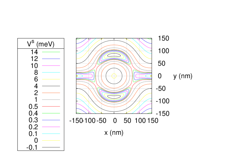
The quantum ring is embedded in the central system of length $L_{x}=300$ nm situated between two contact areas that will be coupled to the external leads, as is depicted in Fig. 5. The system potential is described by

with the parameters from table 1, which are selected such that the potential is a bit higher at the contact regions (the place where electrons tend otherwise to accumulate) than at the ring arms to guarantee a uniform density distribution along the ring. $x_{03}=\epsilon$ is a small numerical symmetry breaking parameter and $|\epsilon|=10^{-5}$ nm is enough for numerical stability. In Eq. (64), $\hbar\Omega_{0}=1.0$ meV is the characteristic energy of the confinement and $m^{*}=0.067m_{e}$ is the effective mass of an electron in GaAs-based material. The ring radius $a\approx 80$ nm, which means that $\alpha\approx x_{R}\times 7.1$ meV nm.

The Hamiltonian for the semi-infinite lead $l\in\{L,R\}$ (left or right lead),

with the momentum operator containing only the kinetic momentum and the vector potential coming from the magnetic field (i.e. no photon field)

We remind the reader that the Rashba part, $\hat{H}_{R}(\mathbf{r})$, (Eq. (8)) and Dresselhaus part, $\hat{H}_{D}(\mathbf{r})$, (Eq. (9)) of the spin-orbit interaction are momentum dependent and it is the momentum from Eq. (66), which is used for these terms in Eq. (65). Equation (65) contains the lead field operator

in the two-component vector

and a corresponding definition of the hermitian conjugate to Eq. (4). In Eq. (67), $\psi_{ql}(x)$ is a SES in the lead $l$ (eigenstate with quantum number $q$ of Hamiltonian Eq. (65)) and $\hat{C}_{ql}$ is the associated electron annihilation operator. The lead potential

confines the electrons parabolically in $y$-direction. We use a relatively strong confinement, $\hbar\Omega_{l}=2.0$ meV, to reduce the number of subbands in the leads and thereby the computational effort for our total time-dependent quantum system.

We use the time-convolutionless generalized master equation [50] TCL-GME, which is a non-Markovian master equation that is local in time. This master equation satisfies the positivity conditions [63] for the MB state occupation probabilities in the RDO usually to a higher system-lead coupling strength [9]. We assume, the initial total statistical density matrix can be written as a product of the system and leads density matrices, before switching on the coupling to the leads,

with $\rho_{l}$, $l\in\{L,R\}$, being the normalized density matrices of the leads. The coupling Hamiltonian between the central system and the leads reads

References

- [1] Y. Aharonov and D. Bohm, Phys. Rev. 115, 485 (1959).
- [2] Y. Aharonov and A. Casher, Phys. Rev. Lett. 53, 319 (1984).
- [3] Y. Aharonov and J. Anandan, Phys. Rev. Lett. 58, 1593 (1987).
- [4] M. V. Berry, Proc. R. Soc. Lond. A 392, 45 (1984).
- [5] B. Szafran and F. M. Peeters, Phys. Rev. B 72, 165301 (2005).
- [6] S. S. Buchholz, S. F. Fischer, U. Kunze, M. Bell, D. Reuter, and A. D. Wieck, Phys. Rev. B 82, 045432 (2010).
- [7] M. Büttiker, Y. Imry, and M. Y. Azbel, Phys. Rev. A 30, 1982 (1984).
- [8] K. N. Pichugin and A. F. Sadreev, Phys Rev. B 56, 9662 (1997).
- [9] T. Arnold, C.-S. Tang, A. Manolescu, and V. Gudmundsson, Phys. Rev. B 87, 035314 (2013).
- [10] H.-F. Cheung, Y. Gefen, E. K. Riedel, and W.-H. Shih, Phys. Rev. B 37, 6050 (1988).
- [11] W.-C. Tan and J. C. Inkson, Phys. Rev. B 60, 5626 (1999).
- [12] R. A. Webb, S. Washburn, C. P. Umbach, and R. B. Laibowitz, Phys. Rev. Lett. 54, 2696 (1985).
- [13] S. Oh and C.-M. Ryu, Phys. Rev. B 51, 13441 (1995).
- [14] Y. A. Bychkov and E. I. Rashba, Journal of Physics C: Solid State Physics 17, 6039 (1984).
- [15] G. Dresselhaus, Phys. Rev. 100, 580 (1955).
- [16] D. Loss, P. Goldbart, and A. V. Balatsky, Phys. Rev. Lett. 65, 1655 (1990).
- [17] A. V. Balatsky and B. L. Altshuler, Phys. Rev. Lett. 70, 1678 (1993).
- [18] A. A. Kovalev, M. F. Borunda, T. Jungwirth, L. W. Molenkamp, and J. Sinova, Phys. Rev. B 76, 125307 (2007).
- [19] S. K. Maiti, M. Dey, S. Sil, A. Chakrabarti, and S. N. Karmakar, EPL (Europhysics Letters) 95, 57008 (2011).
- [20] M. Nita, D. C. Marinescu, A. Manolescu, and V. Gudmundsson, Phys. Rev. B 83, 155427 (2011).
- [21] E. B. Sonin, Phys. Rev. Lett. 99, 266602 (2007a).
- [22] Q.-f. Sun, X. C. Xie, and J. Wang, Phys. Rev. B 77, 035327 (2008).
- [23] J. S. Sheng and K. Chang, Phys. Rev. B 74, 235315 (2006).
- [24] A. Matos-Abiague and J. Berakdar, Phys. Rev. Lett. 94, 166801 (2005).
- [25] Y. V. Pershin and C. Piermarocchi, Phys. Rev. B 72, 245331 (2005).
- [26] O. V. Kibis, Phys. Rev. Lett. 107, 106802 (2011).
- [27] O. V. Kibis, O. Kyriienko, and I. A. Shelykh, Phys. Rev. B 87, 245437 (2013).
- [28] Z.-G. Zhu and J. Berakdar, Phys. Rev. B 77, 235438 (2008).
- [29] O. Jonasson, C.-S. Tang, H.-S. Goan, A. Manolescu, and V. Gudmundsson, New Journal of Physics 14, 013036 (2012).
- [30] E. Jaynes and F. W. Cummings, Proceedings of the IEEE 51, 89 (1963).
- [31] Y. Wu and X. Yang, Phys. Rev. Lett. 98, 013601 (2007).
- [32] A. T. Sornborger, A. N. Cleland, and M. R. Geller, Phys. Rev. A 70, 052315 (2004).
- [33] D. Frustaglia and K. Richter, Phys. Rev. B 69, 235310 (2004).
- [34] G. Ying-Fang, Z. Yong-Ping, and L. Jiu-Qing, Chinese Physics Letters 21, 2093 (2004).
- [35] A. G. Aronov and Y. B. Lyanda-Geller, Phys. Rev. Lett. 70, 343 (1993).
- [36] Y.-S. Yi, T.-Z. Qian, and Z.-B. Su, Phys. Rev. B 55, 10631 (1997).
- [37] X. F. Wang and P. Vasilopoulos, Phys. Rev. B 72, 165336 (2005).
- [38] C. S. Tang and C. S. Chu, Phys. Rev. B 60, 1830 (1999).
- [39] G. Zhou and Y. Li, J. Phys.: Condens. Matter 17, 6663 (2005).
- [40] J.-W. Jung, K. Na, and L. E. Reichl, Phys. Rev. A 85, 023420 (2012).
- [41] C. S. Tang and C. S. Chu, Physica B 292, 127 (2000).
- [42] G. Zhou, M. Yang, X. Xiao, and Y. Li, Phys. Rev. B 68, 155309 (2003).
- [43] H. Spohn, Rev. Mod. Phys. 52, 569 (1980).
- [44] S. A. Gurvitz and Y. S. Prager, Phys. Rev. B 53, 15932 (1996).
- [45] N. G. van Kampen, Stochastic Processes in Physics and Chemistry, 2nd ed. (North-Holland, Amsterdam, 2001).
- [46] U. Harbola, M. Esposito, and S. Mukamel, Phys. Rev. B 74, 235309 (2006).
- [47] C. Bruder and H. Schoeller, Phys. Rev. Lett. 72, 1076 (1994).
- [48] A. Braggio, J. König, and R. Fazio, Phys. Rev. Lett. 96, 026805 (2006).
- [49] V. Moldoveanu, A. Manolescu, and V. Gudmundsson, New Journal of Physics 11, 073019 (2009).
- [50] H.-P. Breuer, B. Kappler, and F. Petruccione, Phys. Rev. A 59, 1633 (1999).
- [51] T. Arnold, M. Siegmund, and O. Pankratov, Journal of Physics: Condensed Matter 23, 335601 (2011).
- [52] W.-C. Tan and J. C. Inkson, Semiconductor Science and Technology 11, 1635 (1996).
- [53] J. Shi, P. Zhang, D. Xiao, and Q. Niu, Phys. Rev. Lett. 96, 076604 (2006).
- [54] N. Bray-Ali and Z. Nussinov, Phys. Rev. B 80, 012401 (2009).
- [55] E. I. Rashba, Phys. Rev. B 68, 241315 (2003).
- [56] H.-J. Drouhin, G. Fishman, and J.-E. Wegrowe, Phys. Rev. B 83, 113307 (2011).
- [57] F. Bottegoni, H.-J. Drouhin, G. Fishman, and J.-E. Wegrowe, Phys. Rev. B 85, 235313 (2012).
- [58] E. B. Sonin, Phys. Rev. B 76, 033306 (2007b).
- [59] F. E. Meijer, A. F. Morpurgo, and T. M. Klapwijk, Phys. Rev. B 66, 033107 (2002).
- [60] B. Molnár, F. M. Peeters, and P. Vasilopoulos, Phys. Rev. B 69, 155335 (2004).
- [61] N. Byers and C. N. Yang, Phys. Rev. Lett. 7, 46 (1961).
- [62] S. Viefers, P. Koskinen, P. S. Deo, and M. Manninen, Physica E: Low-dim. Systems and Nanostr. 21, 1 (2004).
- [63] R. S. Whitney, J. Phys. A: Math. Theor. 41, 175304 (2008).
- [64] V. Gudmundsson, O. Jonasson, C.-S. Tang, H.-S. Goan, and A. Manolescu, Phys. Rev. B 85, 075306 (2012).
- [65] V. Gudmundsson, C. Gainar, C.-S. Tang, V. Moldoveanu, and A. Manolescu, New Journal of Physics 11, 113007 (2009).
- [66] See Supplemental Material at [URL will be inserted by publisher] for the time- and space-dependence of the spin current densities without photon cavity and of the spin photocurrent densities of photon field polarization . The spin polarization , the Rashba coefficient meV nm and the Dresselhaus coefficient . A vector of length corresponds to .