Radiation Magnetohydrodynamics In Global Simulations Of Protoplanetary Disks.
Abstract
Aims. Our aim is to study the thermal and dynamical evolution of protoplanetary disks in global simulations, including the physics of radiation transfer and magneto-hydrodynamic turbulence caused by the magneto–rotational instability.
Methods. We develop a radiative transfer method based on the flux-limited diffusion approximation that includes frequency dependent irradiation by the central star. This hybrid scheme is implemented in the PLUTO code. The focus of our implementation is on the performance of the radiative transfer method. Using an optimized Jacobi preconditioned BiCGSTAB solver, the radiative module is three times faster than the magneto–hydrodynamic step for the disk setup we consider. We obtain weak scaling efficiencies of up to cores.
Results. We present the first global 3D radiation magneto-hydrodynamic simulations of a stratified protoplanetary disk. The disk model parameters are chosen to approximate those of the system AS 209 in the star-forming region Ophiuchus. Starting the simulation from a disk in radiative and hydrostatic equilibrium, the magneto–rotational instability quickly causes magneto–hydrodynamic turbulence and heating in the disk. We find that the turbulent properties are similar to that of recent locally isothermal global simulations of protoplanetary disks. For example, the rate of angular momentum transport is a few times . For the disk parameters we use, turbulent dissipation heats the disk midplane and raises the temperature by about compared to passive disk models. The vertical temperature profile shows no temperature peak at the midplane as in classical viscous disk models. A roughly flat vertical temperature profile establishes in the disk optically thick region close to the midplane. We reproduce the vertical temperature profile with a viscous disk models for which the stress tensor vertical profile is flat in the bulk of the disk and vanishes in the disk corona.
Conclusions. The present paper demonstrates for the first time that global radiation magneto–hydrodynamic simulations of turbulent protoplanetary disks are feasible with current computational facilities. This opens up the windows to a wide range of studies of the dynamics of protoplanetary disks inner parts, for which there are significant observational constraints.
Key Words.
Protoplanetary disks, accretion disks, Magnetohydrodynamics (MHD), radiation transfer, Methods: numerical1 Introduction
The understanding of planet formation requires a deep insight into the physics of protoplanetary disks. Recent observations of young disks in nearby star-forming regions (Furlan et al., 2009; Andrews et al., 2009) have been able to constrain important physical parameters, like the disk mass and radial extent, its flaring index or the dust–to–gas mass ratio. Our understanding of these observations is mainly based on 2D radiative viscous disk models (Chiang & Goldreich, 1997; D’Alessio et al., 1998; Dullemond et al., 2002) that include proper dust opacities and irradiation by the star. The energy released by the accretion process is an important source for determining the structure and the evolution of the inner disk regions. The magneto-rotational instability (Balbus & Hawley, 1998, MRI,) is the most likely candidate to drive accretion by an effective viscosity from magnetic turbulence. Up to now there is no global model which combines both magneto-hydrodynamics (MHD) turbulence driven by the MRI and the radiative transfer including irradiation by the star and proper dust opacities. The main challenge to perform such simulations is the computational effort. Global MHD simulations need high resolutions to resolve the MRI properly (Fromang & Nelson, 2006; Flock et al., 2010; Sorathia et al., 2012) and the computational cost required to solve additional radiative transfer equations remains a challenge. The first full radiation magneto-hydrodynamics (RMHD) of that problem were performed in local box simulations by Turner et al. (2003) using a flux-limited diffusion (FLD) approach (Levermore & Pomraning, 1981). In the past few years, several accretion disk simulations have been performed using similar numerical schemes (Turner, 2004; Hirose et al., 2006; Blaes et al., 2007; Krolik et al., 2007; Flaig et al., 2009) and recently including irradiation heating (Hirose & Turner, 2011). More sophisticated radiation hydrodynamics (RHD) methods, like the two-moment method (González et al., 2007) are usually very time demanding because they require large matrix inversion. In this work we develop a radiative transfer method based on the two-temperature grey11 1 A grey approach integrates over all frequencies FLD approach by Commerçon et al. (2011) and including frequency dependent irradiation by the star (Kuiper et al., 2010). This hybrid scheme captures accurately the irradiation energy by the star and performs well compared to computational expensive Monte-Carlo radiative transfer methods (Kuiper & Klessen, 2013). We particularly focus on the serial and parallel performance of our method. The model we design is especially suited for global RMHD disk calculations. Our paper is split into the following parts. In section 2 we describe the RMHD equations, the numerical scheme and a performance test. In section 3 we explain our initial conditions for global RMHD disk calculations, the iteration method for calculating the disks radiative hydrostatic equilibrium and the boundary conditions. In section 4 we present the results, followed by the discussion and the conclusion. In the Appendix we show details of the discretization of the FLD method, the numerical developments and tests.
2 Numerical implementations
2.1 Equations and numerical scheme
In this paper we solve the ideal RMHD equations using the FLD approximation and including irradiation by a central star. We use a spherical coordinate system which has advantages for the treatment of stellar irradiation by means of a simple ray-tracing approach and because it is well adapted to the flared structure of protoplanetary disks. The set of equations reads
| (1) | |||||
| (2) | |||||
| (3) | |||||
| (4) | |||||
| (5) |
in which the two coupled equations for the radiation transfer are
| (6) | |||||
| (7) |
with the density , the velocity vector , the magnetic field vector22 2 The magnetic field is normalized over the factor , the total pressure , the gas pressure with the gas temperature , the mean molecular weight , the Boltzmann constant , the atomic mass unit , the gravitational potential with the gravitational constant G, stellar mass , r the radial distance to the star, the total energy with the gas internal energy , the radiation energy ER, the irradiation flux , the Rosseland and Planck mean opacity and , the radiation constant with the Stefan-Boltzmann constant erg.cm-2s-1K-4, and c the speed of light. To enforce causality, we use the flux limiter by Levermore & Pomraning (1981, Eq. 28 therein) with . The closure relation between gas pressure and internal energy is provided by the ideal gas equation of state , with the adiabatic index . We choose a mixture of hydrogen and helium with solar abundance (Decampli et al., 1978; Bitsch et al., 2013a) so that and .
After the MHD step, the method solves the two-coupled radiative transfer equations (6 and 7). We neglect in the equations all terms of the order (Krumholz et al., 2007), including the radiation pressure terms and the radiation force in the momentum equations since . These approximations are well suited for our applications () but not necessarily for other regimes, like the dynamic diffusion (Krumholz et al., 2007). A similar method was presented in Bitsch et al. (2013b) or Kolb et al. (2013).
It has recently been shown that frequency dependent irradiation is more accurate in the context of protoplanetary disks to capture irradiation heating (Kuiper et al., 2010; Kuiper & Klessen, 2013). The irradiation flux at a radius is calculated as
| (8) |
with the Planck function , the solid angle , the surface temperature of the star , the radius of the star , the frequency , and the radial optical depth for the irradiation flux
| (9) |
The irradiation by the star is used as a source term in Eq. 3. This approximation is valid due to short penetration time for stellar rays through the domain compared to the longer hydrodynamical timescale.
Fig. 1 shows the frequency dependent dust absorption opacity. The opacity tables are derived for particle sizes of 1 and below (Draine & Lee, 1984). We note that for the setup presented in this paper the temperature stays below the dust evaporation temperature of about 1000 K so that we can neglect the gas opacities. To calculate the opacity involved in the RMHD equations we take into account the dust–to–gas mass ratio for small particles which we define as 1% of the total dust–to–gas mass ratio (Birnstiel et al., 2012).
The ideal MHD equations are solved using the PLUTO code (Mignone, 2009). The PLUTO code is a highly modular, multidimensional and multi-geometry code that can be applied to relativistic or non-relativistic (magneto-)hydrodynamics flows. For this work we choose the Godunov type finite volume configuration which consists of a second order space reconstruction, a second order Runge-Kutta time integration, the constrained transport (CT) method (Gardiner & Stone, 2005), the orbital advection scheme FARGO MHD (Masset, 2000; Mignone et al., 2012), the HLLD Riemann solver (Miyoshi & Kusano, 2005), and a Courant number of . In this work we neglect the magnetic dissipation which would appear at the right hand side of Eq. 5. The effect of magnetic dissipation is discussed in the conclusion section.
To solve Eq. (6 and 7) we use an implicit method as the gas velocities are small compared to the speed of light. The implicit discretized equations in spherical coordinates can be found in the Appendix. We rewrite the radiative transfer equations in the matrix form where x is the solution vector. The solution of this system involves a matrix inversion and is solved by an iterative method to minimize the residual until a given accuracy is reached. We use the Jacobi-preconditioned BiCGSTAB solver based on the work by Van der Vorst (1992). As a convergence criteria we use the reduction of the norm of the residual, .

2.2 Radiative transfer method validation


As a validation of our algorithm, we perform the radiation transfer test for disks described by Pascucci et al. (2004). We compute the equilibrium temperature spatial distribution of a static disk irradiated by a star using different radiative transfer methods. We compare our method results with the one obtained using the Monte-Carlo radiative transfer code RADMC-3D33 3 www.ita.uni-heidelberg.de/˜dullemond/software/radmc-3d (Dullemond, 2012). Following Pascucci et al. (2004), we use the opacity table of Draine & Lee (1984), a dust–to–gas mass ratio of , and frequency dependent irradiation with frequency bins. The star parameters are with and . The gas density follows
| (10) |
with
| (11) |
We present here the most optically thick disk configuration of Pascucci et al. (2004) for which g.cm-3. The initial temperature is set to K. The domain size ranges from to AU in radius and from to in . We use a grid with logarithmically increasing cell size in radius and uniform in . The overall grid contains cells. The boundary conditions of the radiation energy are fixed to K in the poloidal direction and zero gradient in the radial direction. We solve the radiative transfer equations with a fixed time-step until we reach thermal equilibrium. The convergence criterion is . In RADMC-3D we use photons. We plot the temperature profile over radius and height in Fig. 2. Both profiles agree very well with the results by RADMC-3D. In the Appendix A.2, we describe a resolution study of this test to determine the order of the scheme. We also perform an additional diffusion test for our FLD method that we present for completeness.
2.3 Serial and parallel performance

An important emphasis of our work was to develop a module with high computational efficiency. During the development we focused on reducing the number of operations per iteration cycle of the implicit method. By increasing the memory usage we improved substantially the performances of the algorithm. We performed an analysis of our module for the fiducial disk model (see section 4). The MHD part takes while the radiation module consumes of a full RMHD step. In our module each matrix vector multiplications per iteration in the BiCGSTAB method have the main computational cost with from the full RMHD step, followed by the frequency dependent irradiation with . In the following we present a weak scaling test. The number of iterations by the matrix solver is fixed to 30 which is a typical value for reaching convergence in our global high resolution model. We use cells per cpu as in this model, for which we use cores. Fig. 3 shows the parallel performance of the RMHD module using an Intel Xeon 2.27 Ghz system. With cores we reach a scaling efficiency of 70.3 which is acceptable given the non-local nature of the algorithm. Nevertheless, the parallel performance is lower than the pure Godunov scheme (Mignone et al., 2007). This is largely due to the important amount of communications inside the BiCGSTAB method. Here one has to distribute three times all neighboring cells for each core per iteration to compute the new residual. As the number of iterations strongly depends on the physical problem, we do not a priori know the serial and the parallel performance for a given application beforehand. We note that the parallel performance depends also on the ratio between the number of grid cells to communicate over the grid cells per core. Reducing the number of cells below per core would result in reduced scaling performances.
3 Initial disk structure and boundary conditions
As an illustration of the possibilities offered by our numerical implementation of a FLD scheme within the PLUTO code, we present in the remaining of this paper a series of 3D RMHD simulations of a fully turbulent protoplanetary disk. In this section, we describe the disk model parameters and the iterative procedure we design to construct an initial setup that is in hydrostatic equilibrium. Boundary conditions in these simulations turned out to be subtle, so we also detail the set of conditions we used in this particular case. We caution the reader that finding a proper set of boundary conditions is delicate and likely to be problem dependent.
3.1 An iterative procedure
Finding an irradiated disk structure in hydrostatic equilibrium is not a straightforward task. This is because, for a given irradiation source, the disk temperature depends on the spatial density distribution which itself depends on temperature (because of the pressure force). We thus solve for the hydrostatic disk structure iteratively: assuming a given density in the disk, we calculate the temperature as a result of disk irradiation using the hybrid FLD module described above. To calculate the new radiation and temperature field we use the typical diffusion time for this problem. The diffusion time can be estimated by . Using typical values at 1 AU with solar parameters g.cm-3, cm2 g-1 and AU, we obtain s. After the temperature and radiation field have reached equilibrium, a new density profile is calculated and the algorithm iterates until convergence.
The following input parameters are needed: the surface density over radius , the opacity including the dust-to-gas mass ratio and the stellar parameters T∗, M∗, and R∗. The density and the azimuthal velocity are updated integrating the equations of hydrostatic equilibrium in spherical coordinates using a second order Runge Kutta method. In hydrostatic equilibrium, these are, for the radial and poloidal direction respectively
| (12) | |||||
| (13) |
Once is known for a given value of (e.g. for the midplane) and for all , Eq. (12) can be used to calculate . The second equation is then integrated to give the density field at the next interface for any value of and we can repeat the cycle. Using the mid-point integral method we reach second order accuracy. We impose the midplane gas density using
| (14) |
where and . The above relation is only valid for a constant vertical temperature and so a Gaussian vertical density profile. We do not expect this to be the case here since the temperature can a priori vary with distance to the midplane. However, the bulk of the disk around the midplane has a constant vertical temperature (see Fig. 4 and section 3.2 below). Since this is the location where most of the mass is located, the actual surface density is close to the targeted value with small deviations of . To reach a higher accuracy, we multiply the density in each grid cell by a constant factor so that we reach the target value before calculating the new temperature. We iterate the procedure until both the temperature and density field have converged to better than , where is the number of iterations step. A validation of this iterative method is presented in Appendix B by reproducing the passive disk model of Chiang & Goldreich (1997).
3.2 Simulations parameters: the case of AS 209


We use the scheme detailed above to calculate the initial disk structure of the series of simulations we present in section 4. We choose stellar and disk parameters inspired from those of the circumstellar disk AS 209 in the Ophiuchus star-forming region, for which there are a number of observational constraints (Koerner & Sargent, 1995; Andrews et al., 2009; Pérez et al., 2012). Stellar mass, radius, and surface temperature are well constrained parameters and we adopt the same values as Andrews et al. (2009) with 0.9 M☉, 2.3 R☉, and 4250 K. The gas surface density in the inner region of AS 209 is nearly a free parameter and only constrained indirectly by the dust surface density. Andrews et al. (2009) estimated for this system a total dust surface density (including all particle sizes) of less than g.cm-2 at 1 AU from the star.
For radiation hydrodynamics, the distribution of the small particles ( m) is most important. This is because these particles dominate the opacity at optical, near- and mid-infrared wavelengths. They contain most of the dust surface, which is the controlling parameter for the opacity. By contrast, most of the dust mass, is stored in larger particles (Birnstiel et al., 2012). Roughly speaking, the dust surface density of the small particles can be estimated to be less than g.cm-2, using the parameters by Andrews et al. (2009). We have calculated our disk structure for three different amounts of small size dust particles: g.cm-2. The initial temperature distribution in radiative hydrostatic equilibrium for the three cases is shown in Fig. 4. In the top panel, g.cm-2 and the disk displays a large optical thick region. In the bottom panel, having g.cm-2, we find a very extended heated upper region while the disk midplane is completely optically thin to its own thermal radiation. Between these two extrema we choose our fiducial model with a dust surface density of g.cm-2. In this configuration (shown on the middle panel of Fig. 4), both an optically thick midplane and an extended optically thin corona fit within the computational domain. The gas surface density is set to g.cm, such that it equals the minimum mass solar nebula (MMSN) value at AU but displays a shallower slope than the MMSN such as suggested by Andrews et al. (2009), even if those constraints come from larger radial distances. Assuming again that small particles carry only 1% of the total dust mass, we obtain a total dust–to–gas mass ratio of in our fiducial model.
The simulation spans the radial range AU, the poloidal range , and the azimuthal range . For the fiducial model in initial equilibrium, we obtain at which results in scale heights fitting in the computational domain at its inner boundary. Due to the disk flaring the value of at the outer radius is larger, with corresponding to scale heights at the outer boundary.
3.3 Boundary conditions
Finding suitable boundary conditions for a stable and physically reasonable global simulation such as presented in this paper is already difficult in ideal MHD. Radiative transfer makes the problem even more difficult. In this section we describe in detail the boundary conditions we have designed for that purpose. Straightforward periodic boundary conditions are used for all variables in the azimuthal direction, so we focus on the radial and poloidal boundaries.
In the radial direction we extrapolate linearly the density and azimuthal velocity. Radial and poloidal velocities are all set to zero gradient. In the case of inflowing gas with a Mach number of or higher, we force the radial velocity boundary condition to be reflective. The poloidal and toroidal magnetic field components are set to follow a profile, while the radial magnetic field is calculated to ensure in the ghost cells. Temperature is set to zero gradient and we use for the radiation energy density with being the initial radiative hydrostatic equilibrium temperature. In order to avoid irradiation from directly illuminating the first radial cell of the computational domain, we set a vertical dependent optical depth with the subscript 0 corresponding to the first cell in the radial direction. Using six stellar radii as the inner disk edge is a reasonable approximation to absorb most of the irradiation at the disk midplane, as would be done by the inner parts of the disk44 4 Young stellar objects have dominant magnetic fields inside a few stellar radii, which destroy the disc structure (Günther, 2013). Accordingly, the Rosseland opacity at the radial boundary is modified in the optically thick region so that . Even if this boundary condition seems unrealistic it will prevent an artificial pile up of the radiation energy density near the boundary, and so permits the correct disk flaring (see Appendix B).
In the poloidal direction we force the density to drop exponentially. The velocities are set to zero gradient. In case of inflowing poloidal velocities we reflect in the ghost cells. Tangential magnetic fields are set to zero gradient, while we calculate the poloidal field so as to enforce . The temperature is set to zero gradient and the radiation energy density is fixed to with K. The temperature in the poloidal direction has to be small to ensure the disk can cool by radiating its energy away.
4 Results
| Model | Resolution | Radius:: | Method | Orbits | |||
|---|---|---|---|---|---|---|---|
| L3D | 256x64x256 | 0.5-1.5: 0.13: | RMHD | 0-650 | |||
| 256x64x256 | 0.5-1.5: 0.13: | RMHD | 0-650 | ||||
| H3D | 512x128x512 | 0.5-1.5: 0.13: | RMHD | 0.076 | 300-600 | ||
| H3D-ISO | 512x128x512 | 0.5-1.5: 0.13: | MHD | 0.044 | 300-600 | ||
| H2D | 512x128x1 | 0.5-1.5: 0.13: | RHD | - | 0-200 | ||
| 512x128x1 | 0.5-1.5: 0.13: | RHD | - | 0-200 |
Table 1 summarizes the models we performed and provides an overview of the integrated angular momentum transport properties we obtain. Models and are low resolution RMHD simulations, with . Such a low resolution enables long integration times of about 650 inner orbits. While the dust–to–gas mass ratio in model is equal to our fiducial value, , it is reduced by one order of magnitude in model . To save computational time, we interpolate the results of model after 300 inner orbits on a grid twice as fine. After this time, the MRI has saturated, and we use the interpolated magnetic fields to restart the simulation, which constitutes model . This represents the fiducial model of the present paper and is described in detail in the following sections. In Appendix C we describe the procedure of interpolation and restarting. To connect with previous work, its properties are compared with model H3D-ISO which is a locally isothermal model that uses an azimuthal- and time-averaged temperature profile calculated from the results of model (see section 4.2). Finally, we compare our results with a couple of 2D radiative hydrodynamic simulations (performed in the disk poloidal plane) of viscous disks, namely models and , that use different prescriptions for the viscous stress tensor (see section 4.1.2). All MHD simulations are initialized with a pure toroidal magnetic field with a uniform plasma beta value . Initial random velocity fluctuations are added to the initial disk configuration with an amplitude equal to of the local speed of sound.
4.1 Model H3D
4.1.1 Turbulent properties


We start with a general description of the integrated properties of the turbulence in model . The turbulent nature of the flow is best illustrated by Fig. 5 which shows two snapshots of the gas velocity fluctuations and the magnetic field strength in the disk. The root–mean–squared (RMS) velocities in the disk midplane range from 1 m.s-1 up to 100 m.s-1. In the corona the turbulent velocities increase above 1000 m.s-1. This is consistent with the azimuthal and time averaged vertical profile of the gas turbulent velocities as shown in Fig. 6 (black curve). When normalized by the local sound speed (blue curve), the plot shows a local Mach number around at the midplane. This is typical of values obtained in isothermal simulations (Fromang & Nelson, 2006; Flock et al., 2010). However, in contrast with such simulations, the turbulent Mach number reaches a peak (with roughly sonic velocity fluctuations) at around , which corresponds to around two pressure scale heights. The Mach number then decreases above the peak location as the temperature (and so the sound speed) rises faster than the turbulent velocity.
The right panel of Fig. 5 shows the magnetic field strength spatial distribution. In the midplane, it ranges from Gauss up to Gauss. In the corona, the field shows larger and smoother fluctuations with values below Gauss. That magnetic field is largely responsible for angular momentum radial transport in the disk. In Fig. 7, we plot the vertical profile of the accretion stress which is the sum of Reynolds and Maxwell stresses
| (15) |
where is the radial and azimuthal velocity fluctuations and represents the time average. The black curve corresponds to the absolute values of the stress (in cgs units). It displays a peak of dyn.cm-2 at about , a plateau with a small drop close to the midplane ( dyn.cm-2), and decreases in the disk corona. Such a profile is in qualitative agreement with results of isothermal local simulations (Simon et al., 2012) as well as in radiative MHD local simulations (Hirose et al., 2006; Flaig et al., 2010), and in locally isothermal global MHD simulation (Fromang & Nelson, 2006). By normalizing the stress over the local pressure (blue curve), we also obtain a vertical profile and absolute values similar to isothermal simulations (Flock et al., 2011). amounts to about in the disk equatorial plane and increases up to a few times in the corona. Table 1 further shows the value of the accretion stress volume averaged over the entire computational domain. Following Flock et al. (2011), its normalized value is defined according to
| (16) |
Time average is done between 400 and 500 inner orbits. Again, we find typical values of about a few times , very similar to transport coefficients measured in locally isothermal global simulations of turbulent protoplanetary disks in the last few years. We note that the changes in the turbulence properties over radius remain small during the simulation. Nevertheless, there are regions of increased activity. This is the case for example of the region that is about AU broad visible in the 3D snapshots close to AU at the midplane (Fig. 5), where turbulent velocities and magnetic fields are larger. Such zones of increased turbulent activity could be connected to long-lived zonal flows such as observed in local (Johansen et al., 2009; Dittrich et al., 2013) and global simulations (Dzyurkevich et al., 2010; Flock et al., 2011) when using an isothermal equation of state. We now move in the following to the specificities of the present work that are associated with radiative transfer.
4.1.2 Temperature evolution


The time–averaged vertical temperature profile at AU in model H3D is shown in Fig. 8 and compared with the temperature vertical profile at the start of the simulation (i.e., when the disk is in hydrostatic equilibrium). As a consequence of turbulent heating, the disk midplane temperature increases from around 140 K to 160 K for model H3D. This corresponds to an increase of the disk pressure scale height of 7 %. The temperature profile is flat in the optically thick part of the disk and rising in its upper layers due to the stellar irradiation. At those locations, we find a small reduction of the temperature by a few percents (bottom panel of Fig. 8). This is because the disk vertical density profile is flattened in the upper layers as a result of magnetic support (Hirose & Turner, 2011, in agreement with previous results, see for example ). This shields the disk corona from the incoming irradiation at a given height compared to the initial model and leads to a small drop in the temperature.
We next investigate whether such a vertical temperature profile can be accounted for in the framework of standard -disk models. We perform an axisymmetric 2D RHD simulation (model H2D) in the disk poloidal plane using a constant viscosity with and the local sound speed . The 2D model is initialized using azimuthally averaged values of the density, pressure, temperature, azimuthal velocity, and radiation energy density as obtained in model H3D. The temperature in the 2D viscous RHD model quickly relaxes into a steady state that is overplotted on the top panel of Fig. 8. As we see, a classical disk prescription does not reproduce the correct midplane temperature. It predicts a midplane temperature of about K, higher than that of model H3D and does not display the flat temperature profile in the optically thick part of the disk. Here, most of the heat is released at the midplane vicinity due to the scaling of the viscous stress tensor with density. By contrast, the turbulent stress tensor in our simulation is rather flat for (see Fig. 7) with variations of only a factor of . We thus perform an additional 2D RHD simulation, model , that uses a different prescription for viscosity55 5 , with and being the midplane density value, such that the viscous stress tensor remains constant with height below scale heights while it vanishes above that location. This prescription to model the turbulence in one or two dimensional simulation has been used by Kretke & Lin (2010); Landry et al. (2013). The vertical temperature profile we obtain in that model is also shown in Fig. 8. It shows midplane temperature and vertical profile in much better agreement with the full 3D RMHD model H3D. Besides the gas temperature one can define the radiation temperature as . In Fig. 9 we plot the vertical profile of both temperatures after 480 inner orbits. In the optically thick midplane, the two temperatures are well coupled due to the high opacity. In the optically thin upper layers the two temperatures start to diverge due to the irradiation. The radiation temperature stays at the level of the midplane value. Fig. 9 shows also the temperature fluctuations (red dotted line). The fluctuations are small. The maximum relative temperature fluctuations are close to the line of the irradiation with values between and . In Fig. 10 we plot the time evolution of the azimuthally averaged total stress over height. The blue contour lines show the peak of stress at each time. They follow the butterfly motions of the mean toroidal field which is triggered by the MRI dynamo (Gressel, 2010). The peak of relative temperature fluctuations are close to the azimuthally averaged absorption layer of the irradiation (white line). It suggests that the peak of relative temperature fluctuations is triggered by the fluctuations of the surface.
4.1.3 Heating and cooling rates


In this section we take a closer look at the heating and cooling rates in the RMHD model H3D. To do so, we proceed as follows: over any given timestep, we recorded the change of the internal energy that occurred during the MHD step, as well as the change of internal energy that occurred during the radiative step. The former captures all dynamical heating and cooling mechanisms, including the advection of energy or the transfers from kinetic, magnetic or gravitational energy into thermal energy (see Eq. 3). We then sum these fractional internal energy changes (divided by the timestep and multiplied by the corresponding cell volume) over a large time interval to compute the heating and cooling rates associated with dynamical and radiative processes. These are respectively labelled and . Fig. 11 shows meridional snapshots of both quantities, respectively on the left () and right () panels. Both quantities are azimuthally and time averaged over 40 inner orbits starting after 380 inner orbits. The plots show that most of the disk is being heated with a rate in the order of that is mostly released in the disk upper layers, . This corresponds to around two pressure scale heights above the disk midplane. Radiative cooling (bottom panel) roughly balances that heating, showing the disk is approximately in steady state. In order to investigate how much of that heat can be attributed to turbulent dissipation, we calculate the expected theoretical heating rate , following Balbus & Papaloizou (1999). Fig. 12, left, shows a meridional snapshot of the turbulent heating that can be computed according to
| (17) |
The vertical profiles of the heating rates, plotted in Fig. 12 right, show a good correlation between and . Most of the disk heating can be attributed to MHD turbulence locally dissipated into heat and only in the upper disk layers, part of the energy is transported away by waves.
4.2 Effect of resolution, equation of state and dust–to–gas mass ratio


We have focused so far on the high resolution model H3D. However, both the vertical profile of the turbulent stress and the turbulent velocity depend on several factors of numerical and physical nature.
First of all, the spatial resolution of the grid is known to be of importance. This is a particularly constraining problem in global simulations. Recently the convergence and the effect of resolution in global adiabatic (Hawley et al., 2013) and locally isothermal (Parkin & Bicknell, 2013) simulations were investigated. A convergence study in fully radiative global simulations is difficult to achieve and would go beyond the scope of this paper. As a first step in that direction, we nevertheless present the results of model L3D in which the resolution is half compared to model H3D. In this low resolution simulations, there are seven grid cells per pressure scale height. This is not enough to resolve properly the MRI (Flock et al., 2010; Sorathia et al., 2012) which leads to a reduction of the total accretion stress. The normalized total accretion stress varies between for model and for model . As shown in Fig. 13, the stress vertical profiles of in both models are significantly different. At the midplane the stress in model L3D drops by one order of magnitude. This is expected as in stratified MRI simulation it becomes more difficult to resolve properly the MRI at the midplane due to its low magnetization (Fromang & Nelson, 2006; Flock et al., 2011).
Second, the isothermal model H3D-ISO shows a reduced stress compared to the full RMHD model H3D. It decreases from to . Such a trend of increased turbulence in radiative models was also suggested by Flaig et al. (2010). Nevertheless, as shown in Fig. 13, the vertical profile of the stress has a similar shape for both models.
The last effect we want to discuss is the influence of the dust–to–gas mass ratio. In model , we reduce it by one order of magnitude to . As shown on Fig. 4, this shifts the irradiated hotter disk region down to the midplane. In Fig. 14, we plot the temperature profiles at 1 AU, averaged over azimuth and time between 200 and 400 inner orbits. As the disk becomes hotter, the sound speed increases and a higher saturation level of the MRI is expected (Balbus & Hawley, 1998). An effect of increased turbulence can be seen by comparing model (dashed line) and model (dashed–dotted line) in Fig. 13: the vertical profile of model , shows an overall larger stress than model . The total normalized stress is increased by 25%, see Table 1. But more important is the position of the maximum stress. The hotter temperature region has shifted by down to the midplane, but the peak stress is still located at . This result indicates again that the position of the maximum stress due to MRI is independent of the vertical temperature profile. This position seems also independent of resolution by comparing model and model .
The position of the maximum of the stress is connected to the plasma beta. The vertical profiles of for the models and are shown in Fig. 15, using the same time and space average. Even if the temperature profiles are quite different, the plasma beta value drops at the same height () in both models. All these results indicate that the vertical shape and especially the location of the peak of MRI turbulent magnetic fields are independent from the vertical temperature profile.
5 Conclusion and future work
In this paper, we successfully implemented in the PLUTO code a FLD method in spherical coordinates, including frequency dependent irradiation by a star. It is well adapted to performing global simulations of irradiated accretion disks such as protoplanetary disks. The FLD module has serial performances that are three times faster than the MHD part even for a mainly optically thin disk setup. We performed the first global 3D radiation magneto-hydrodynamics simulations of an irradiated and turbulent protoplanetary disk. The disk parameters were inspired by that of the system AS 209 in the star-forming region Ophiuchus (Andrews et al., 2009) for which there are strong observational constraints. The simulations started from a radiative hydrostatic disk which becomes MRI unstable, turbulent, and finally develops into a steady state with typical values of a few times , comparable to published simulations of the same kind that use a locally isothermal equation of state. We investigated the turbulent properties and compared the disk structure with classical viscous disk models. Our findings are:
- •
The vertical temperature profile showed no temperature peak at the midplane as in classical viscous disk models (D’Alessio et al., 1998). A roughly flat vertical temperature profile established in the disk optically thick region close to the midplane. We reproduced the midplane temperature from the full 3D RMHD run using 2D viscous disk simulations in which the stress tensor is constant in the bulk of the disk and vanishes in the disk corona. A simple prescription is given with the turbulent stress being constant in the vertical direction within two pressure scale heights of the midplane, and vanishing above. Such a simple prescription gives a satisfying account of the results.
- •
The main heating in the turbulent disks was dominated by the stress tensor. We observed a heating of the order of erg.s-1, mainly released in the disk upper heights.
- •
The temperature fluctuations in the disk were small and of the order of 1%. A small increase was observed close to the transition region where the disk got heated by the irradiation from the star with fluctuations up to 6%.
- •
The turbulent magnetic fields reached field strengths of about to Gauss at the midplane. The turbulent velocity of the gas was around to m/s at the midplane, and up to 1000 in the disk upper heights.
We want to point out some limitations of our work. The first one is the distribution and abundance of small sized dust particles. Indeed, the latter strongly affects the disk temperature vertical profile (see Fig. 4). For our model we choose the disk AS 209, which has a relative low dust abundance compared to other protostellar systems (Andrews et al., 2009). For the dust surface density we used g.cm-2 at AU for grain sizes m. A much larger amount of small sized dust is difficult to include as it needs a much larger vertical extent to obtain the optical thin irradiated region. At the same time such large extents in stratified MHD turbulent simulation are difficult to perform. In our simulations we used a fixed dust–to–gas mass ratio. In contrast, a smaller dust amount over most of the disk height is expected in weakly turbulent disks, e.g. (Zsom et al., 2011; Akimkin et al., 2013). All these points show that the total amount and distribution of small dust particles is rather uncertain. These simulations should be thought of as a proof of concept that RMHD simulations of turbulent protoplanetary disks are now feasible given the current computational resources.
Another limitation is our use of the ideal MHD approximation. It is well known that the electron fraction is so low at AU in protoplanetary disks that dissipation terms (Ohmic resistivity, ambipolar diffusion, and Hall term) are important (Okuzumi & Hirose, 2011; Bai, 2011; Dzyurkevich et al., 2013). These dissipative processes are expected to stabilize the MRI in the bulk of the disk, producing a laminar dead zone around the disk equatorial plane (Gammie, 1996). The presence of a dead zone and the consequences of the various dissipative processes at play will mainly affect the vertical profiles of the turbulent stress and heating rate (Hirose & Turner, 2011). These are key aspects of protoplanetary disks dynamics that should be included in future simulations performed in the planet forming regions of protoplanetary disks.
Our current implementation assumes that the gas and dust temperatures are perfectly coupled. Recent models by Akimkin et al. (2013) predict photoelectric heating as a dominant heating source for the gas affected by UV flux. We thus expect that the gas temperature and even the dust temperature (Akimkin et al., 2011) to be higher in the irradiated regions than presently estimated in our models. Detailed studies of the flow in the corona (for example reconnection and heating events) should include this effect to be meaningful. This would be the purpose of future developments of our numerical scheme.
Acknowledgements
We thank Rolf Kuiper for several helpful comments and discussion during this project. We thank Andrea Mignone for supporting us with the newest PLUTO code including the FARGO advection scheme. Parallel computations have been performed on the Genci supercomputer ’curie’ at the calculation center of CEA TGCC. The research leading to these results has received funding from the European Research Council under the European Union’s Seventh Framework Programme (FP7/2007-2013) / ERC Grant agreement nr. 258729.
Appendix A Flux–limited–diffusion method
A.1 Numerical scheme
We discretize the equations (6-7) in spherical coordinates using a finite volume formulation and a fully implicit scheme
| (18) | |||
| (19) | |||
with the specific heat capacity , the geometrical terms , , , , and the irradiation flux . Equations A.1 and A.2 are coupled by linearizing the term proportional to that appears in both equations and neglecting the high order term (Commerçon et al., 2011)
| (20) |
This approximation is valid if the change of the temperature is small. The maximum change of the relative temperature per time-step during our RMHD disk simulations is always below . Using this expression we can combine Equations A.1 and A.2 and construct the matrix that needs to be inverted. We note that in this version the scheme is first order in time due to the first-order backward Euler step, used for the time integration.
A.2 Test in spherical geometry
A.2.1 Diffusion test
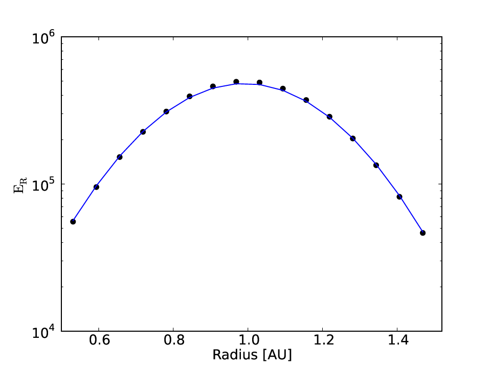


In this section we test the diffusion operator in spherical coordinates
| (21) |
We set up a domain of with different resolutions of , , and . We use a logarithmic increasing grid in radius so that . The domain is shifted in the direction, to test all the geometrical terms. As initial conditions we use the Gauss function
with and the Cartesian position vector . The position is placed at , and . is fixed to and to g.cm-3. We set the flux limiter to , the initial time to s and the boundary conditions to the analytical value for the given time. We evolve until . The timestep for the model is set to which represents a Courant number 66 6 The Courant number for a parabolic problem is defined as . of . The timestep is decreased by a factor of 4 each time the resolution is doubled to keep the Courant number constant. Fig. 16 presents the profile of along each direction for the low resolution case, left column, and the profile of the relative error for each direction and resolution, right column. The low resolution run matches with the analytical profile with relative error around 2%. We remind that this test problem is difficult to handle in spherical coordinates due to the different grid spacing and especially the change of the volume over radius. As this test problem is time dependent, we observe a first-order convergence rate which is expected, using a first-order time integration (Jiang et al., 2012).
A.2.2 Full hybrid scheme
In this second test we repeat the equilibrium setup, see section 2.2, to determine the order of the full hybrid scheme and to verify the equilibrium temperature in the low resolution case. We perform a resolution study using five different resolutions , , , and . In this test we set the convergence criteria to . Fig. 17, left, shows the vertical temperature profile at 2 AU for the different resolutions. Even the lowest resolution (blue dots) matches very well with the reference solution (black solid line). The temperature profile from the highest resolution is taken as reference temperature . The order of the scheme can be tested by comparing the norm as a function of the grid spacing. We define the norm as
| (22) |
with the number of cells for a given coarse resolution, the temperature and the corresponding volume of the coarse grid cell and , and the temperature and volume of the highest resolution run and . We average the reference temperature over the given volume of the coarse resolution. Using this volume average becomes here important as the method and so the divergence terms are written in the finite volume approach, see Eq. 19. In Fig. 17, right, we show the norm (black dots) overplotted with the theoretical slope of a second order scheme. As this test problem is time independent, we are able to obtain second order space accuracy. We note that the irradiation, the heating source, is only radius dependent and so a one dimensional problem.
Appendix B Validation of radiative hydrostatic equilibrium
In this section we test the iterative method presented in section 3.1. To do so, we compare the hydrostatic disk structure we obtained using that procedure for a given set of disk parameters with the simple model described by Chiang & Goldreich (1997). The disk parameters, chosen to match that work, are as follows: , , , g.cm-2, where stands for the distance to the star in astronomical units. We fix the opacity to . We use a logarithmically increasing grid with cells. The radial domain extends from to AU and the poloidal domain covers the range . We follow the iteration procedure presented in section 3.1 to compute the hydrostatic structure of that disk. The resulting 2D radiative hydrostatic temperature profile is plotted in Fig. 18. The black solid line in Fig. 18 shows the location of the photosphere.
As mentioned, some of the basic properties of irradiated disks can be well estimated using the model of Chiang & Goldreich (1997), the basic physics of which we review here. The disk is irradiated at the photosphere . The heating at that location by the incoming irradiation can be written
| (23) |
where is the irradiated surface element at the disk surface. If we assume isotropic blackbody cooling at the photosphere we can write the cooling as
| (24) |
Since irradiation hits the disk surface with a small angle one can approximate (in other words, most of the cooling is done through disk emission in the vertical direction). Assuming that heating and cooling balance each other, we find (see also Chiang & Goldreich, 1997, Eq. (1))
| (25) |
The term is often called the flaring angle and can be expressed as
| (26) |
Using Eq. (26), we can calculate the flaring angle of our disk model and derive the expected equilibrium temperature in our model using Eq. (25). In Fig. 19 (top panel), we plot the temperature in the corona (red dotted line at ) and in the midplane (red solid line), overplotted with the corresponding blackbody temperature (black dotted line) and the equilibrium temperature (black solid line). The two curves we obtained using our iterative procedure are in good agreement with the approximate expressions provided by the Chiang & Goldreich (1997) model.
In fig. 19 (bottom panel), we plot in addition the disk scale height over radius. When combining Eq. (26) with the Gaussian vertical profile of the disk (in the case of an isothermal disk), a simple formulae for its radial profile is obtained (Chiang & Goldreich, 1997):
| (27) |
This analytical prediction is confronted on the bottom panel of fig. 19 (solid line) with our numerical estimate of the same quantity. Again, the agreement between the two curves validates our iterative procedure.


Appendix C Restarting H3D model
As mentioned, we restarted our high resolution model from a magnetic field configuration after MRI saturation from model L3D. This requires interpolating the simulation data from a coarse grid to a refined grid (with refined cells between twice as small as the coarse cells). In MHD, this is not an immediate procedure if one wants to retain the solenoidal nature of the magnetic field. In the constraint transport MHD method, the magnetic fields are located at cells interfaces. Coarse cells interfaces are refined, and the magnetic field on those refined surfaces is simply injected from those coarse cell interfaces. In addition, new interfaces appear in the refined grid that do not exist in the coarse grid. At those locations, we perform a linear interpolation of and we use that interpolation to reconstruct the new magnetic field. This ensures on the refined grid.
Having the magnetic field at high resolution, we restart the model first with pure isothermal MHD using the initial density and temperature profiles derived from hydrostatic equilibrium. We let the system relax for around 1000 steps. Then we take the velocities and the magnetic fields from the relaxed state, but the density and temperature profiles again from the hydrostatic equilibrium. Restarting from this with full radiative RMHD will result after around 10 outer orbits into a new saturated state avoiding the linear MRI phase.
References
- Akimkin et al. (2013) Akimkin, V., Zhukovska, S., Wiebe, D., et al. 2013, ApJ, 766, 8
- Akimkin et al. (2011) Akimkin, V. V., Pavlyuchenkov, Y. N., Vasyunin, A. I., et al. 2011, Ap&SS, 335, 33
- Andrews et al. (2009) Andrews, S. M., Wilner, D. J., Hughes, A. M., Qi, C., & Dullemond, C. P. 2009, ApJ, 700, 1502
- Bai (2011) Bai, X.-N. 2011, ApJ, 739, 50
- Balbus & Hawley (1998) Balbus, S. A. & Hawley, J. F. 1998, Reviews of Modern Physics, 70, 1
- Balbus & Papaloizou (1999) Balbus, S. A. & Papaloizou, J. C. B. 1999, ApJ, 521, 650
- Birnstiel et al. (2012) Birnstiel, T., Klahr, H., & Ercolano, B. 2012, A&A, 539, A148
- Bitsch et al. (2013a) Bitsch, B., Boley, A., & Kley, W. 2013a, A&A, 550, A52
- Bitsch et al. (2013b) Bitsch, B., Crida, A., Morbidelli, A., Kley, W., & Dobbs-Dixon, I. 2013b, A&A, 549, A124
- Blaes et al. (2007) Blaes, O., Hirose, S., & Krolik, J. H. 2007, ApJ, 664, 1057
- Chiang & Goldreich (1997) Chiang, E. I. & Goldreich, P. 1997, ApJ, 490, 368
- Commerçon et al. (2011) Commerçon, B., Teyssier, R., Audit, E., Hennebelle, P., & Chabrier, G. 2011, A&A, 529, A35
- D’Alessio et al. (1998) D’Alessio, P., Canto, J., Calvet, N., & Lizano, S. 1998, ApJ, 500, 411
- Decampli et al. (1978) Decampli, W. M., Cameron, A. G. W., Bodenheimer, P., & Black, D. C. 1978, ApJ, 223, 854
- Dittrich et al. (2013) Dittrich, K., Klahr, H., & Johansen, A. 2013, ApJ, 763, 117
- Draine & Lee (1984) Draine, B. T. & Lee, H. M. 1984, ApJ, 285, 89
- Dullemond (2012) Dullemond, C. P. 2012, RADMC-3D: A multi-purpose radiative transfer tool, astrophysics Source Code Library
- Dullemond et al. (2002) Dullemond, C. P., van Zadelhoff, G. J., & Natta, A. 2002, A&A, 389, 464
- Dzyurkevich et al. (2010) Dzyurkevich, N., Flock, M., Turner, N. J., Klahr, H., & Henning, T. 2010, A&A, 515, A70
- Dzyurkevich et al. (2013) Dzyurkevich, N., Turner, N. J., Henning, T., & Kley, W. 2013, ApJ, 765, 114
- Flaig et al. (2009) Flaig, M., Kissmann, R., & Kley, W. 2009, MNRAS, 282
- Flaig et al. (2010) Flaig, M., Kley, W., & Kissmann, R. 2010, MNRAS, 409, 1297
- Flock et al. (2010) Flock, M., Dzyurkevich, N., Klahr, H., & Mignone, A. 2010, A&A, 516, A26
- Flock et al. (2011) Flock, M., Dzyurkevich, N., Klahr, H., Turner, N. J., & Henning, T. 2011, ApJ, 735, 122
- Fromang & Nelson (2006) Fromang, S. & Nelson, R. P. 2006, A&A, 457, 343
- Furlan et al. (2009) Furlan, E., Watson, D. M., McClure, M. K., et al. 2009, ApJ, 703, 1964
- Gammie (1996) Gammie, C. F. 1996, ApJ, 457, 355
- Gardiner & Stone (2005) Gardiner, T. A. & Stone, J. M. 2005, Journal of Computational Physics, 205, 509
- González et al. (2007) González, M., Audit, E., & Huynh, P. 2007, A&A, 464, 429
- Gressel (2010) Gressel, O. 2010, MNRAS, 404
- Günther (2013) Günther, H. M. 2013, Astronomische Nachrichten, 334, 67
- Hawley et al. (2013) Hawley, J. F., Richers, S. A., Guan, X., & Krolik, J. H. 2013, ApJ, 772, 102
- Hirose et al. (2006) Hirose, S., Krolik, J. H., & Stone, J. M. 2006, ApJ, 640, 901
- Hirose & Turner (2011) Hirose, S. & Turner, N. J. 2011, ApJ, 732, L30
- Jiang et al. (2012) Jiang, Y.-F., Stone, J. M., & Davis, S. W. 2012, ApJS, 199, 14
- Johansen et al. (2009) Johansen, A., Youdin, A., & Klahr, H. 2009, ApJ, 697, 1269
- Koerner & Sargent (1995) Koerner, D. W. & Sargent, A. I. 1995, AJ, 109, 2138
- Kolb et al. (2013) Kolb, S. M., Stute, M., Kley, W., & Mignone, A. 2013, ArXiv e-prints
- Kretke & Lin (2010) Kretke, K. A. & Lin, D. N. C. 2010, ApJ, 721, 1585
- Krolik et al. (2007) Krolik, J. H., Hirose, S., & Blaes, O. 2007, ApJ, 664, 1045
- Krumholz et al. (2007) Krumholz, M. R., Klein, R. I., McKee, C. F., & Bolstad, J. 2007, ApJ, 667, 626
- Kuiper et al. (2010) Kuiper, R., Klahr, H., Dullemond, C., Kley, W., & Henning, T. 2010, A&A, 511, A81
- Kuiper & Klessen (2013) Kuiper, R. & Klessen, R. S. 2013, A&A, 555, A7
- Landry et al. (2013) Landry, R., Dodson-Robinson, S. E., Turner, N. J., & Abram, G. 2013, ApJ, 771, 80
- Levermore & Pomraning (1981) Levermore, C. D. & Pomraning, G. C. 1981, ApJ, 248, 321
- Masset (2000) Masset, F. 2000, A&AS, 141, 165
- Mignone (2009) Mignone, A. 2009, Nuovo Cimento C Geophysics Space Physics C, 32, 37
- Mignone et al. (2007) Mignone, A., Bodo, G., Massaglia, S., et al. 2007, ApJS, 170, 228
- Mignone et al. (2012) Mignone, A., Flock, M., Stute, M., Kolb, S. M., & Muscianisi, G. 2012, A&A, 545, A152
- Miyoshi & Kusano (2005) Miyoshi, T. & Kusano, K. 2005, Journal of Computational Physics, 208, 315
- Okuzumi & Hirose (2011) Okuzumi, S. & Hirose, S. 2011, ApJ, 742, 65
- Parkin & Bicknell (2013) Parkin, E. R. & Bicknell, G. V. 2013, ArXiv e-prints
- Pascucci et al. (2004) Pascucci, I., Wolf, S., Steinacker, J., et al. 2004, A&A, 417, 793
- Pérez et al. (2012) Pérez, L. M., Carpenter, J. M., Chandler, C. J., et al. 2012, ApJ, 760, L17
- Simon et al. (2012) Simon, J. B., Beckwith, K., & Armitage, P. J. 2012, MNRAS, 422, 2685
- Sorathia et al. (2012) Sorathia, K. A., Reynolds, C. S., Stone, J. M., & Beckwith, K. 2012, ApJ, 749, 189
- Turner (2004) Turner, N. J. 2004, ApJ, 605, L45
- Turner et al. (2003) Turner, N. J., Stone, J. M., Krolik, J. H., & Sano, T. 2003, ApJ, 593, 992
- Van der Vorst (1992) Van der Vorst, H. A. 1992, SIAM J. Sci. and Stat. Comput, 13, 631–644
- Zsom et al. (2011) Zsom, A., Ormel, C. W., Dullemond, C. P., & Henning, T. 2011, A&A, 534, A73