$\Lambda(1405)$ photoproduction based on chiral unitary model

First we define kinematical variables. We consider the $\gamma(q)+p(p)\to K^{+}(k)+\pi(k_{\pi})+\Sigma(p^{\prime})$ reaction in which the variables in the parentheses are four-momenta for the particles in the total center-of-mass system. The differential cross section for the reaction is derived following a standard procedure, and given as

where $M_{p}$, $M_{\Sigma}$, $m_{K^{+}}$ and $m_{\pi}$ are the masses of the proton, $\Sigma$, $K^{+}$ and $\pi$, respectively, and the Källen function is denoted by $\lambda(x,y,z)$. The symbol $s$ is the squared total energy of the system, and is related to the four-momenta by $s=W^{2}=(q+p)^{2}=(k+k_{\pi}+p^{\prime})^{2}$, while the invariant mass of the $\pi\Sigma$ subsystem is $M^{2}_{\pi\Sigma}=(k_{\pi}+p^{\prime})^{2}$. The kinematical variables with asterisk stand for the quantities in the $\pi\Sigma$ center-of-mass system. The summation of spin and polarization states in initial and final particles are indicated by $\sum_{\rm spin}$; the average factor, 1/4, for the initial states is already included in the factor of the formula. All information about the dynamics is encoded into the reaction amplitude $T_{K^{+}\pi\Sigma,\gamma p}$ in Eq. (1), and is discussed in detail in the next subsection. The line-shape of the $\pi\Sigma$ spectrum is obtained by integrating Eq. (1) over the angular part of $\vec{p}^{\prime*}$ and $\vec{k}$, and given as

As stated in the introduction, we describe the $\gamma p\to K^{+}\pi\Sigma$ reaction by a set of tree-level mechanisms for $\gamma p\to K^{+}M_{j}B_{j}$ ($M_{j}B_{j}$ : a set of meson and baryon) followed by $M_{j}B_{j}\to\pi\Sigma$ rescattering. We use an index $j=1,...,10\,$ to specify $M_{j}B_{j}=K^{-}p,\bar{K}^{0}n,\pi^{0}\Lambda,\pi^{0}\Sigma^{0},\eta\Lambda,\eta\Sigma^{0}$, $\pi^{+}\Sigma^{-},\pi^{-}\Sigma^{+},K^{+}\Xi^{-},K^{0}\Xi^{0}$, respectively. Thus the reaction amplitude introduced in Eq. (1), $T^{j}\equiv T_{K^{+}M_{j}B_{j},\gamma p}$, is given by

where $V^{j}_{\alpha}$ is a tree-level photo-production mechanism. In the next paragraph, we specify the tree mechanisms that go into our calculation. The summation of $\alpha$ runs over all of the tree-level photoproduction mechanisms included in our calculation. Contribution from the rescattering is denoted by $T^{j}_{R}$. The rescattering amplitude is calculated with a partial wave expansion with respect to the relative motion of $M_{j}B_{j}$, and $(J,L)=(1/2,0)$ and $(1/2,1)$ partial waves are considered; $J$ and $L$ are the total and orbital angular momenta for $M_{j}B_{j}$. The partial wave amplitude is given, with the on-shell factorization, by

where $T^{j}_{R;JL}$ and $V^{j}_{\alpha;JL}$ are partial wave amplitudes of $T^{j}_{R}$ and $V^{j}_{\alpha}$, respectively, and are calculated with the on-shell momenta of relevant particles. More details about the partial wave expansion, including the relation between $T^{j}_{R;JL}$ and $T^{j}_{R}$, are given in Appendix A. For the $M_{j^{\prime}}B_{j^{\prime}}\to M_{j}B_{j}$ scattering amplitudes $T^{jj^{\prime}}_{JL}$, we use those from the chiral unitary model given in Ref. [20] for $(J,L)=(1/2,0)$ wave, and in Ref. [21] for $(J,L)=(1/2,1)$ wave. The $(J,L)=(1/2,0)$ wave contains $\Lambda(1405)$ as double poles, while the $(J,L)=(1/2,1)$ wave does not include any resonance and provide a smooth background. It is turned out that the contribution from the $(J,L)=(1/2,1)$ wave rescattering is small. We use the meson-baryon Green function, $G^{j}_{\alpha}$, calculated with the dimensional regularization as follows:

where $M_{B_{j}}$ and $M_{M_{j}}$ are the masses of a baryon $B_{j}$ and a meson ${M_{j}}$, respectively, and we use the values listed in the Particle Data Group [22] for the masses. The relative on-shell momentum of $M_{j}B_{j}$ corresponding to $s$ is denoted by $\bar{q}_{j}$. The symbol $a^{j}_{\alpha}(\mu)$ is the subtraction constant for the regularization scale $\mu$, and we set $\mu=630$ MeV for all channels. The subtraction constants can depend on a channel $j$ as well as a production mechanism $\alpha$; we will come back to this point at the end of this section.

We consider gauge-invariant tree-level photo-production mechanisms ($V^{j}_{\alpha}$) as follows: minimal substitution to the lowest order chiral meson-baryon interaction such as the Weinberg-Tomozawa terms (Fig. 1) and the Born terms (Fig. 2); vector-meson exchange mechanisms (Fig. 3).

Thus, for specifying each mechanism $\alpha$, we use the label for each figure in Figs. 1-3 so that $\alpha=$ 1(a), 1(b), .., 3(k). These photo-production mechanisms are expanded in terms of $1/M_{B}$, and ${\cal O}(1)$ and ${\cal O}(1/M_{B})$ terms are considered in our calculation. Explicit expressions for $V^{j}_{\alpha}$, as well as our model Lagrangians from which $V^{j}_{\alpha}$ are derived, are shown in Appendix B and C. Coupling constants contained in $V^{j}_{\alpha}$ of Figs. 1-3 are fixed either by data (other than $\gamma p\to K^{+}\pi\Sigma$) if possible, or by SU(3) relation if poorly constrained by data. More details about the couplings are given in Appendix B.

With the meson-exchange production mechanisms and the subtraction constants ($a^{j}_{\alpha}(\mu)$ in Eq. (5)) taken as the same as those in the chiral unitary amplitudes, we cannot reproduce the $\pi\Sigma$ line-shape data for the $\gamma p\to K^{+}\pi\Sigma$ reaction from the CLAS [8]. Therefore, it is inevitable to introduce adjustable degrees of freedom to fit the data. Thus all of the meson-exchange mechanisms $V^{j}_{\alpha}$ are multiplied by a common form factor of the following form:

where $\bm{k}^{*}$ and $\bm{k}_{j}^{*}$ are respectively the momenta of $K^{+}$ and $M_{j}$ in the center-of-mass frame of $M_{j}B_{j}$. The cutoff $\Lambda$ will be used to fit the data. In addition, we also consider phenomenological contact terms that can simulate mechanisms not explicitly considered, such as, in particular, $N^{*}$ and $Y^{*}$ excitation mechanisms. We take couplings for the contact terms $W$-dependent ($W$ : total energy of the system), and will be determined by fitting the $\gamma p\to K^{+}\pi\Sigma$ data [8]. We consider three types of contact terms that are gauge-invariant at the tree-level, and are couple to $K^{+}\bar{K}N$ and $K^{+}\pi\Sigma$ states of different charges, and thus we have 15 complex couplings at each $W$. Expressions for the contact terms are presented in Eqs. (99)-(101) in Appendix. Also, for the mechanism index $\alpha$, we write $\alpha=c1,c2,c3$, as in Eqs. (99)-(101). The form factor of Eq. (6) is not applied to the contact terms.

The subtraction constants $a^{j}_{\alpha}(\mu)$ included in Eq. (5) are also adjusted to fit the data, thereby changing the interference pattern between different production mechanisms. As already stated, $a^{j}_{\alpha}(\mu)$ can depend on the production mechanism $\alpha=$ 1(a), 1(b), .., 3(k), $c1,c2,c3$. However, some of $\alpha$’s should have the same value for $a^{j}_{\alpha}(\mu)$. Also, we do not want to have too many free parameters from the subtraction constants, because it will complicate fitting the data. Thus we classify the production mechanisms into several groups, and each group has its own real subtraction constant. In grouping, we try to classify important mechanisms into different groups so that we have effective freedom in fitting. In TABLE 1, we show the classification of the mechanisms into 11 groups labeled by A,B,…,K.

The subtraction constant for each group is denoted by $a^{j}_{\alpha^{\prime}}(\mu)$ where ${\alpha^{\prime}}$ refers to one of the groups, A,B,…,K. Then $a^{j}_{\alpha^{\prime}}(\mu)$ will be used to fit the data [8]. It is noted that we do not adjust the subtraction constants in the chiral unitary amplitudes in the fit. The subtraction constants we adjusted are all for the first loop of the rescattering, and for the renormalization of the production mechanism.

For the number of data points to be fitted, we now have rather many free parameters most of which are from contact terms. We find that this amount of degrees of freedom is necessary to obtain a reasonable fit to the data. This situation can be understood, considering that we do not explicitly consider short-range mechanisms (baryon resonances, coupled-channel effects) that will play a substantial role here. Because it will be a very difficult task to identify and/or fix each of the short-range mechanisms, we develop the production model in a practical manner as discussed above. Of course, our method could bring a model-dependence of $\Lambda(1405)$ pole(s) extracted from the data. The model-dependence of $\Lambda(1405)$ pole(s) must be assessed by analyzing the data with different form factors and/or contact terms. This will be a future work.

Before presenting our results, we comment on the calculated quantity to be fitted to the line-shape data from CLAS [8]. In the data analysis done by CLAS in Ref. [8], enhanced events due to the $K^{*}$ peak in the $\pi K^{+}$ invariant mass spectrum has been subtracted. In our model, a mechanism of Fig. 3(i) without rescattering can create the $K^{*}$ peak. Thus we fit the data with the following modified differential cross section:

where ${d\sigma\over dM_{\pi\Sigma}}({\rm full})$ contains all of the meson-exchange mechanisms and contact terms followed by the rescattering as discussed in Sec. II.2, and is calculated using Eq. (2). Meanwhile, the second term ${d\sigma\over dM_{\pi\Sigma}}(V^{\pi\Sigma}_{\ref{fig:vec}({\rm i})})$ contains only the tree-level mechanism of Fig. 3(i). The subtraction in Eq. (7) is done at the cross section level, and the interference between the mechanism of Fig. 3(i) and others is kept to be consistent with the analysis of Ref. [8].

We present all numerical values for the fitting parameters (the cutoff from the form factor, the subtraction constants, and the complex couplings from the contact terms) in Appendix D.

Our results, after the fit, are presented in Fig. 4 where the CLAS data are also shown for comparison.

We fitted the data at $W=2.0$, 2.1, 2.2 and 2.3 GeV. As seen in the figure, our model fits the data very well for all three different charge states of $\pi\Sigma$.

It is interesting to break down the line-shapes into contributions from different mechanisms, as shown in Fig. 5.

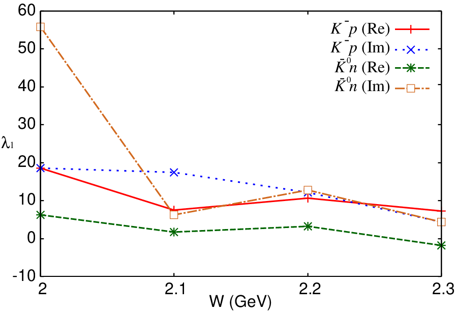
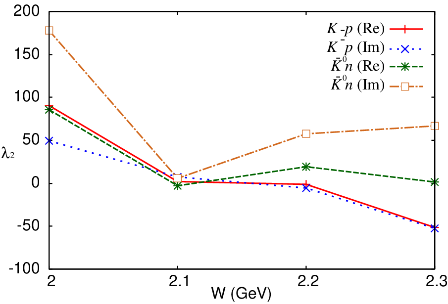
As seen in the figures, different mechanisms gives significant contributions that interfere with each other. We find that the contributions from the gauged Weinberg-Tomozawa terms (Fig. 1) are rather small. In fact, a diagram such as Fig. 1(e) gives a contribution comparable to those from the gauged Born mechanisms (Fig. 2). However, as a result of a destructive interference, the net contribution from the gauged Weinberg-Tomozawa terms is rather small. This destructive interference is not necessarily a result of the gauge invariance. Actually, a dominant term in Fig. 1(e) is gauge invariant itself. Rather, fitting the data have fixed relevant subtraction constants so that the diagrams in Fig. 1 with the rescattering cancel out each other. We find relatively large contributions from mechanisms of Fig. 1(e), 2(b), 2(e), 2(i), 2(l), 3(b), 3(f), that have two propagators rather than three in the other mechanisms; the propagators tend to suppress the contributions of the mechanisms. Meanwhile, the contact terms, which simulate short-range dynamics, also give a large contribution to bring the theoretical calculation into agreement with the data. As seen in TABLE 4, the contact terms have a rather strong coupling to the $\bar{K}N$ channels as a result of the fit. One may find in TABLE 4 that the $W$-dependence of the contact couplings is rather irregular, and is not well under control. However, we note that the contact terms can have a resonant behavior. Also, in Fig. 6, we show the $W$-dependence of the most important contact couplings, $\lambda^{j}_{1}$ and $\lambda^{j}_{2}$ for $j=K^{-}p$ and $\bar{K}^{0}n$. From the figure, it is hard to judge if the behavior of the couplings is out of control. As will be discussed later, however, we would be able to put them under better control if we fit not only the line-shape data but also other observables such as angular distributions. This will be a future work. Finally, we mention that coupled-channels effects are mostly from the $\bar{K}N$ and $\pi\Sigma$ channels.

The difference in the line-shape between different charge states observed in Fig. 4 is a result of the interference between different isospin states. The $\pi\Sigma$ has three isospin states ($I=0,1,2$), and they are separately shown in Fig. 7.

A dominant contribution is from the $I=0$ state as expected due to the $\Lambda(1405)$ peak. The higher mass pole at $1426-16i$ MeV, that creates the prominent bump in the line-shapes, seems to play more important role than the lower mass pole. This is because the production mechanisms in our model generate $\bar{K}N$ more strongly than $\pi\Sigma$, and the final state interaction induces $\bar{K}N\to\pi\Sigma$. As shown in the previous study [12], the higher mass pole couples to the $\bar{K}N$ channel more strongly than the lower mass pole does. The $I=1$ state gives a smaller contribution, still plays an important role to generate the charge dependence of the $\pi\Sigma$ line-shapes. As the energy $W$ increases, the $I=1$ contribution is larger. The $I=2$ state contribution is even more smaller, but still unnegligible. To see this point, we show in Fig. 7 the $\pi^{0}\Sigma^{0}$ line-shape multiplied by 3. The difference between this and the $I=0$ line-shape is the effect of the interference between the $I=0$ and $I=2$ states. We can see that the interference with the $I=2$ state even changes slightly the peak position of the $\pi^{0}\Sigma^{0}$ line-shape.

The different peak positions for differently charged $\pi\Sigma$ states seen in Fig. 4 can be also understood as a result of the interference between a resonant and a background parts. To see this, it is useful to decompose the amplitude into the resonant (second term of Eq. (3)) and background (first term of Eq. (3)) parts. Each of the contributions to $\gamma p\to K^{+}\pi\Sigma$ at $W=2.0$ GeV is shown in Fig. 8.

Interestingly, the background terms give smooth and significant contributions. Although the peak structures are due to the resonant contributions, the background can shift the positions of the peaks, particularly the peak of the $\pi^{0}\Sigma^{0}$ line-shape. After all, the resonant contributions give the peaks at almost the same position, $M_{\pi\Sigma}\sim 1.42$ GeV, for all the differently charged $\pi\Sigma$ states. Thus it seems that one of the $\Lambda(1405)$ poles at $1426-16i$ MeV plays a dominant role in the line-shapes. We will look into this observation in the next subsection.

So far, the excitation of $\Lambda(1405)$ is described by the chiral unitary model, and $\Lambda(1405)$ has the double-pole structure. However, as seen above, only the higher mass pole seems to give the dominant contribution. Thus, it is interesting to see if a single Breit-Wigner can simulate the photo-induced $\Lambda(1405)$ excitation. For this purpose, we use a model in which the rescattering amplitude, $T^{jj^{\prime}}_{JL}$ in Eq. (4), is given by, instead of the chiral unitary amplitude, a single Breit-Wigner function in $(J,L)=(1/2,0)$ and isospin zero partial wave; the other rescattering partial waves amplitudes are set to zero. Here we assume that the rescattering amplitude couples to only $\bar{K}N$ and $\pi\Sigma$ channels. Thus we have

where $M_{BW}$ and $\Gamma_{BW}$ are Breit-Wigner mass and width, respectively. A symbol $C^{BW}_{jj^{\prime}}$ is a complex coupling strength, and will be fitted to the data, along with the Breit-Wigner mass, width and other fitting parameters. Because of being isospin zero, $C^{BW}_{jj^{\prime}}$ have three independent complex values that we denote $C^{BW}_{\bar{K}N,\bar{K}N}$, $C^{BW}_{\bar{K}N,\pi\Sigma}$, and $C^{BW}_{\pi\Sigma,\pi\Sigma}$: $C^{BW}_{\bar{K}N,\bar{K}N}$ is for $(j,j^{\prime})=(1\,{\rm or}\,2,1\,{\rm or}\,2)$; $C^{BW}_{\bar{K}N,\pi\Sigma}$ is for $(j,j^{\prime})\,{\rm or}\,(j^{\prime},j)=(4\,{\rm or}\,7\,{\rm or}\,8,1\,{\rm or}\,2)$; $C^{BW}_{\pi\Sigma,\pi\Sigma}$ is for $(j,j^{\prime})\,=(4\,{\rm or}\,7\,{\rm or}\,8,4\,{\rm or}\,7\,{\rm or}\,8)$. We have defined the index $j$ at the beginning of Sec. II.2. Our Breit-Wigner form of Eq. (8) is more relaxed than the conventional one in which the coupling strengths are related to the width by $\Gamma_{BW}=\sum_{j}\delta(\sqrt{s}-\sqrt{s_{j}})C^{BW}_{jj}$, where the summation is taken over both channels and their particles’ phase-space. In this way, we can simulate non-resonant effects that are not considered explicitly in the rescattering amplitude. The single Breit-Wigner model is fitted to the data and is shown with the data in Fig. 9. The fitted parameters are presented in tables in Appendix D.

Although the quality of the fit is a little worse than the previous model with the chiral unitary amplitude (Fig. 4), still it is an acceptable level. Thus, the line-shape data for $\gamma p\to K^{+}\pi\Sigma$ only do not rule out the possibility of single pole solution for $\Lambda(1405)$. The fit gives $M_{BW}=1412$ MeV and $\Gamma_{BW}=67$ MeV that are close to the middle of the two poles from the chiral unitary amplitude, but still closer to the higher mass pole than to the lower one. As seen in TABLE 5, the Breit-Wigner amplitude couples strongly (weakly) to the $\bar{K}N$ ($\pi\Sigma$) channel, which is also similar to the character of the higher mass pole of $\Lambda(1405)$ in the chiral unitary model.

So far, we fitted only the $\pi\Sigma$ line-shape data for the $\gamma p\to K^{+}\pi\Sigma$ reaction. We found that fitting only the $\pi\Sigma$ line-shape data can lead to several solutions whose quality of the fit to the line-shape data are comparable. However, they can have very different $K^{+}$ angular distribution. Therefore, $K^{+}$ angular distribution data will be useful information to constrain the production mechanism. Recently the CLAS Collaboration reported data for the $K^{+}$ angular distributions [9]. In Figs. 4-8, we actually presented the $\pi\Sigma$ line-shapes from the model that gives $K^{+}$ angular distributions relatively close to the new data of Ref. [9]. Here we use the same model to calculate the $K^{+}$ angular distributions, and show them in Fig. 10.

At $W=2.2$ GeV, our model captures overall trend of the data. However, for the $\gamma p\to K^{+}\pi^{0}\Sigma^{0}$ reaction at $W=2.0$ GeV, there is a sharp rise in the data at $\cos\theta\sim 0$ while rather smooth behavior is found in the calculated counterpart. We actually tried fitting the $K^{+}$ angular distributions data, but this sharply rising behavior cannot be fitted with the current setup. It seems that we need to search for a mechanism that is responsible for this behavior. We leave such a more detailed analysis of the $K^{+}$ angular distribution to a future work.

References

• [1] D.W. Thomas, A. Engler, H.E. Fisk, and R.W. Kraemer, Nucl. Phys. B56, 15 (1973).
• [2] R. J. Hemingway, Nucl. Phys. B253, 742 (1985).
• [3] O. Braun et al., Nucl. Phys. B129, 1 (1977).
• [4] S. Prakhov et al. [Crystal Ball Collaboration], Phys. Rev. C 70, 034605 (2004).
• [5] I. Zychor, M. Buscher, M. Hartmann, A. Kacharava, I. Keshelashvili, A. Khoukaz, V. Kleber and V. Koptev et al., Phys. Lett. B 660, 167 (2008).
• [6] J. K. Ahn [LEPS Collaboration], Nucl. Phys. A 721, 715 (2003).
• [7] M. Niiyama, H. Fujimura, D. S. Ahn, J. K. Ahn, S. Ajimura, H. C. Bhang, T. H. Chang and W. C. Chang et al., Phys. Rev. C 78, 035202 (2008).
• [8] K. Moriya et al. [CLAS Collaboration], Phys. Rev. C 87, 035206 (2013).
• [9] K. Moriya et al. [CLAS Collaboration], Phys. Rev. C 88, 045201 (2013).
• [10] H. Y. Lu et al. [CLAS Collaboration], Phys. Rev. C 88, 045202 (2013).
• [11] As a recent review on the application of the chiral unitary approach to Λ⁡(1405)\Lambda(1405), T. Hyodo and D. Jido, Prog. Part. Nucl. Phys. 67, 55 (2012).
• [12] D. Jido, J. A. Oller, E. Oset, A. Ramos and U. G. Meissner, Nucl. Phys. A 725, 181 (2003).
• [13] T. Hyodo and W. Weise, Phys. Rev. C77, 035204 (2008).
• [14] D. Jido, E. Oset and T. Sekihara, Eur. Phys. J. A 42, 257 (2009).
• [15] L. Roca and E. Oset, Phys. Rev. C 87, 055201 (2013).
• [16] L. Roca and E. Oset, arXiv:1307.5752.
• [17] J.C. Nacher, E. Oset, H. Toki, and A. Ramos Phys. Lett. B455, 55 (1999).
• [18] J. C. Nacher, E. Oset, H. Toki and A. Ramos, Phys. Lett. B 461, 299 (1999).
• [19] B. Borasoy, P. C. Bruns, U. -G. Meissner and R. Nissler, Eur. Phys. J. A 34, 161 (2007).
• [20] E. Oset, A. Ramos, and C. Bennhold, Phys. Lett. B527, 99 (2002).
• [21] D. Jido, E. Oset, and A. Ramos, Phys. Rev. C 66, 055203 (2002).
• [22] J. Beringer et al. (Particle Data Group), Phys. Rev. D 86, 010001 (2012).
• [23] B. C. Pearce and B. Jennings, Nucl. Phys. A528, 655 (1991); T. Sato and T.S.H. Lee, Phys. Rev. C 54, 2660 (1996).
• [24] M. Bando, T. Kugo, K. Yamawaki, Phys. Rep. 164, 217 (1988).
• [25] E. Oset, and A. Ramos, Nucl. Phys. A635, 99 (1998).