Exact sum rules for inhomogeneous systems containing a zero mode

Paolo Amore Email: paolo.amore@gmail.com Address: Facultad de Ciencias, CUICBAS, Universidad de Colima,
Bernal Díaz del Castillo 340, Colima, Colima, Mexico

Abstract

We show that the formulas for the sum rules for the eigenvalues of inhomogeneous systems that we have obtained in two recent papers are incomplete when the system contains a zero mode. We prove that there are finite contributions of the zero mode to the sum rules and we explicitly calculate the expressions for the sum rules of order one and two. The previous results for systems that do not contain a zero mode are unaffected.

Keywords:

Helmholtz equation; inhomogeneous systems;

1 Introduction

In two recent papers, refs. [1, 2], we have derived explicit expressions for the sum rules involving the eigenvalues of inhomogeneous systems described by the Helmholtz equation in a finite region $\Omega$ in $d$ dimensions

\displaystyle(-\Delta)\Psi_{n}(x_{1},\dots,x_{d})=E_{n}\Sigma(x_{1},\dots,x_{d})\Psi_{n}(x_{1},\dots,x_{d})

(1)

where $\Sigma(x_{1},\dots,x_{d})>0$ for $(x_{1},\dots,x_{d})\in\Omega$ . The eigenfunctions $\Psi_{n}(x_{1},\dots,x_{d})$ obey specific boundary conditions on $\partial\Omega$ .

As we have discussed in our previous papers Eq. (1) is isospectral to the equation

\displaystyle\left[\frac{1}{\sqrt{\Sigma(x_{1},\dots,x_{d})}}(-\Delta)\frac{1}{\sqrt{\Sigma(x_{1},\dots,x_{d})}}\right]\Phi_{n}(x_{1},\dots,x_{d})=E_{n}\Phi_{n}(x_{1},\dots,x_{d})\ ,

(2)

while their eigenfunctions are simply related by $\Psi_{n}(x_{1},\dots,x_{d})=\Phi_{n}(x_{1},\dots,x_{d})/\sqrt{\Sigma(x_{1},\dots,x_{d})}$ .

The spectrum of Eqs.(1) and (2) is bounded from below, in some cases being composed by strictly positive eigenvalues while in other cases containing also a zero mode. For example, in the case of an inhomogeneous string, discussed in Ref. [1] a zero mode appears when either Neumann or periodic boundary conditions are enforced.

We briefly describe the procedure that we have devised in our previous work to evaluate the sum rules $Z_{p}=\sum_{n}1/E_{n}^{p}$ , with $p=p_{0},p_{0}+1,\dots$ and $p_{0}$ being the smallest integer for which the series is convergent (in one dimension $p_{0}=1$ ).

We first define the operator

\displaystyle\hat{O}\equiv\frac{1}{\sqrt{\Sigma(x_{1},\dots,x_{d})}}(-\Delta)\frac{1}{\sqrt{\Sigma(x_{1},\dots,x_{d})}}

(3)

appearing in Eq. (2).

The inverse operator may be formally expressed in terms of the Green’s function of the negative Laplacian obeying the same boundary conditions

\displaystyle\hat{O}^{-1}f=\sqrt{\Sigma(x_{1},\dots,x_{d})}\int_{\Omega}G(x_{1},\dots,x_{d},y_{1},\dots,y_{d})\sqrt{\Sigma(y_{1},\dots,y_{d})}f(y_{1},\dots,y_{d})

(4)

Clearly the eigenvalues of this operator are just the reciprocals of the eigenvalues of Eq. (2) (for the moment being we are assuming that the zero mode is not present).

Using the invariance of the trace of an hermitean operator under unitary transformations we are able to relate the spectral sum rules $Z_{p}=\sum_{n}1/E_{n}^{p}$ to the trace of $\hat{O}^{-p}$ , calculated in a suitable basis. We have thus obtained in [1, 2] explicit formulas, which in some cases may be evaluated exactly.

Although this analysis is correct for the cases of problems with a strictly positive spectrum, our previous results are incomplete in the case of a spectrum containing a zero mode, because of additional contributions that we overlooked in our previous calculation. We will now proceed to derive these contributions and then to test them with precise numerical calculations.

In order to avoid the presence of a zero mode we consider the modified operator

\displaystyle\hat{O}_{\gamma}\equiv\frac{1}{\sqrt{\Sigma(x_{1},\dots,x_{d})}}(-\Delta+\gamma)\frac{1}{\sqrt{\Sigma(x_{1},\dots,x_{d})}}

(5)

where $\gamma\rightarrow 0^{+}$ ; similarly we modify Eq. (1) as

\displaystyle(-\Delta+\gamma)\Psi_{n}(x_{1},\dots,x_{d})=E_{n}\Sigma(x_{1},\dots,x_{d})\Psi_{n}(x_{1},\dots,x_{d})

(6)

The trace of $\hat{O}_{\gamma}$ is an invariant under unitary transformations and it may then be evaluated using a suitable basis, as done in the case of problem without a zero mode. Formally the traces of order $p$ , with $p=1,2,\dots$ may be evaluated using the same formulas of Ref.[1, 2], but written in terms of the Green’s function of the shifted negative Laplacian $(-\Delta+\gamma)$

\displaystyle G_{\gamma}(x_{1},\dots,x_{d},y_{1},\dots,y_{d})=\frac{1}{V_{\Omega}\gamma}+\sum_{n}\frac{\phi_{n}(x_{1},\dots,x_{d})\phi_{n}(y_{1},\dots,y_{d})}{\epsilon_{n}+\gamma}

(7)

where $V_{\Omega}$ is the volume of the region $\Omega$ . Here $\epsilon_{n}$ and $\phi_{n}$ are the eigenvalues and eigenfunctions of the negative Laplacian on $\Omega$ obeying specific boundary conditions.

It is possible to expand the Green’s function around $\gamma=0$ as

\displaystyle G_{\gamma}(x_{1},\dots,x_{d},y_{1},\dots,y_{d})=\frac{1}{V_{\Omega}\gamma}+\sum_{q=0}^{\infty}(-1)^{q}\gamma^{q}G^{(q)}(x,y)

(8)

where

\displaystyle G^{(q)}(x,y)\equiv\sum_{n\neq 0}\frac{\phi_{n}(x_{1},\dots,x_{d})\phi_{n}(y_{1},\dots,y_{d})}{\epsilon_{n}^{q+1}}

(9)

Observe that $G^{(0)}(x,y)$ is the regularized Green’s function discussed in [1, 2].

One can easily see that, for $q=1,2,\dots$ ,

\displaystyle(-\Delta_{x})G^{(q)}(x_{1},\dots,x_{d},y_{1},\dots,y_{d})=G^{(q-1)}(x_{1},\dots,x_{d},y_{1},\dots,y_{d})

(10)

and, for $q=0$ ,

\displaystyle(-\Delta_{x})G^{(0)}(x_{1},\dots,x_{d},y_{1},\dots,y_{d})=\delta(x_{1}-y_{1})\dots\delta(x_{d}-y_{d})-\frac{1}{V}

(11)

Using these relations we find

\displaystyle G^{(q+1)}(x_{1},\dots,x_{d},y_{1},\dots,y_{d})\equiv\int d^{d}z\ G^{(0)}(x_{1},\dots,x_{d},z_{1},\dots,z_{d})\ G^{(q)}(z_{1},\dots,z_{d},y_{1},\dots,y_{d})

(12)

which can be straightforwardly verified using the definition (9).

For a finite $\gamma$ these traces provide the sum rules

\displaystyle{\rm Tr}(\hat{O}^{-1}_{\gamma})^{p}=\sum_{n=0}^{\infty}E_{n}^{-p}

(13)

which include the contribution of the zero mode, while the sum rules considered in Refs. [1, 2] are defined as $\lim_{\gamma\rightarrow 0}\sum_{n=1}^{\infty}E_{n}^{-p}$ . We will now show that it is still possible to extract the physical sum rules by properly handling the finite contributions to the trace stemming from the zero mode.

Formally we may write

\displaystyle\sum_{n=1}^{\infty}E_{n}^{-p}=\lim_{\gamma\rightarrow 0}\frac{1}{p!}\frac{\partial^{p}}{\partial\gamma^{p}}\left[\gamma^{p}\left({\rm Tr}(\hat{O}^{-1}_{\gamma})^{p}-\frac{1}{E^{p}_{0}(\gamma)}\right)\right]

(14)

where $E_{0}(\gamma)$ is the energy of the lowest mode, which depends on $\gamma$ ; clearly for $\gamma=0$ the eigenfunction of the fundamental mode of Eq. (6) is $\Psi_{0}=constant$ and therefore $E_{0}(0)=0$ . For an infinitesimal $\gamma$ we expect that both the eigenfunctions and eigenvalues of Eq. (6) have the perturbative expansions $\Psi_{n}(x_{1},\dots,x_{d})=\sum_{r}\gamma^{r}\Psi_{n}^{(r)}(x_{1},\dots,x_{d})$ and $E_{n}=\sum_{r}\gamma^{r}E_{n}^{(r)}$ respectively.

Physically Eq. (14) takes into account the contributions due to the zero mode which are finite for $\gamma\rightarrow 0$ . These contributions are two kinds: the first term in the rhs of the equation contains the contributions due to the finite modification of the trace for $\gamma\rightarrow 0$ , while the second term takes care of eliminating the finite contribution due to $1/E^{p}_{0}(\gamma)$ for $\gamma\rightarrow 0$ . Notice that the divergent contributions due to the zero mode are automatically eliminated.

Let us discuss explicitly the simplest case of the sum rule of order $p=1$ for an inhomogeneous string. In this case

\displaystyle{\rm Tr}(\hat{O}^{-1}_{\gamma})={\rm Tr}\left[\left(\frac{1}{V_{\Omega}\gamma}+\sum_{q=0}^{\infty}(-1)^{q}\gamma^{q}G^{(q)}\right)\Sigma\right]

(15)

The finite part of this expression is just

\displaystyle\lim_{\gamma\rightarrow 0}\frac{\partial}{\partial\gamma}\gamma{\rm Tr}(\hat{O}^{-1}_{\gamma})={\rm Tr}\left[G^{(0)}\Sigma\right]

(16)

and it coincides with the expression in Ref. [1]. However in order to obtain the sum rule we also need to subtract the finite contribution of the zero mode. To do this we need to evaluate $E_{0}(\gamma)$ to order $\gamma^{2}$ and use it to obtain

\displaystyle\frac{1}{E_{0}(\gamma)}=\frac{1}{E_{0}^{(1)}\gamma+E_{0}^{(2)}\gamma^{2}+\dots}=\frac{1}{E_{0}^{(1)}\gamma}-\frac{E_{0}^{(2)}}{\left(E_{0}^{(1)}\right)^{2}}+O(\gamma)

(17)

Using the perturbative approach described in A we obtain:

	$\displaystyle\frac{1}{E_{0}}$	$\displaystyle=$	$\displaystyle\frac{\left(\int_{\Omega}\Sigma(x_{1},\dots,x_{d})d^{d}x\right)}{V_{\Omega}\gamma}$		(18)
		$\displaystyle+$	$\displaystyle\frac{\int_{\Omega}d^{d}x\int_{\Omega}d^{d}y\Sigma(x_{1},\dots,x_{d})G^{(0)}(x_{1},\dots,x_{d},y_{1},\dots,y_{d})\Sigma(y_{1},\dots,y_{d})}{\left(\int_{\Omega}\Sigma(x_{1},\dots,x_{d})d^{d}x\right)}+O\left(\gamma\right)$		(18)

The finite contribution of the zero mode is therefore

\displaystyle\left.\frac{1}{E_{0}}\right|_{finite}

\displaystyle=

\displaystyle\left(\frac{\int_{\Omega}d^{d}x\int_{\Omega}d^{d}y\Sigma(x_{1},\dots,x_{d})G^{(0)}(x_{1},\dots,x_{d},y_{1},\dots,y_{d})\Sigma(y_{1},\dots,y_{d})}{\left(\int_{\Omega}\Sigma(x_{1},\dots,x_{d})d^{d}x\right)}\right)

(19)

and it needs to be subtracted from the expressions for $Z(1)$ obtained in Ref.[1] for Neumann and periodic bc; in the case of an inhomogeneous string with Neumann bc one has

\displaystyle Z^{(NN)}_{1}=\int_{-a/2}^{a/2}\Sigma(x)\left(\frac{a}{12}+\frac{x^{2}}{a}\right)dx-\frac{\int_{-a/2}^{a/2}dx\int_{-a/2}^{a/2}dy\Sigma(x)G_{NN}^{(0)}(x,y)\Sigma(y)}{\int_{-a/2}^{a/2}dx\Sigma(x)}

(20)

while, for the case of periodic bc one has

\displaystyle Z^{(PP)}_{1}=\int_{-a/2}^{a/2}\frac{a}{12}\Sigma(x)dx-\frac{\int_{-a/2}^{a/2}dx\int_{-a/2}^{a/2}dy\Sigma(x)G_{PP}^{(0)}(x,y)\Sigma(y)}{\int_{-a/2}^{a/2}dx\Sigma(x)}

(21)

Let us now discuss the sum rule of order two; we need the trace

\displaystyle{\rm Tr}(\hat{O}^{-2}_{\gamma})={\rm Tr}\left[\left(\frac{1}{V_{\Omega}\gamma}+\sum_{q=0}^{\infty}(-1)^{q}\gamma^{q}G^{(q)}\right)\Sigma\left(\frac{1}{V_{\Omega}\gamma}+\sum_{q=0}^{\infty}(-1)^{q}\gamma^{q}G^{(q)}\right)\Sigma\right]

(22)

and we extract the finite part of this expression with the limit

\displaystyle\lim_{\gamma\rightarrow 0}\frac{1}{2}\frac{\partial^{2}}{\partial\gamma^{2}}\gamma^{2}{\rm Tr}(\hat{O}^{-2}_{\gamma})={\rm Tr}\left[G^{(0)}\Sigma G^{(0)}\Sigma\right]-\frac{2}{V_{\Omega}}{\rm Tr}\left[\Sigma G^{(1)}\Sigma\right]

(23)

Notice that the first term in the rhs of the equation is the term obtained in Refs. [1, 2]: the second term is due to a finite contribution of the zero mode to the eigenvalues and it involves the Green’s function $G^{(1)}$ .

We have obtained the explicit expressions for $G^{(1)}(x,y)$ for Neumann and periodic bc in one dimension, which read

\displaystyle G_{NN}^{(1)}(x,y)

\displaystyle=

\displaystyle\left\{\begin{array}[]{ccc}\frac{a^{4}-30a^{2}\left(x^{2}-6xy+y^{2}\right)-60a(x-y)^{3}-30\left(x^{4}+6x^{2}y^{2}+y^{4}\right)}{720a}&,&x<y\\ \frac{a^{4}-30a^{2}\left(x^{2}-6xy+y^{2}\right)+60a(x-y)^{3}-30\left(x^{4}+6x^{2}y^{2}+y^{4}\right)}{720a}&,&x>y\\ \end{array}\right.

and

\displaystyle G_{PP}^{(1)}(x,y)

\displaystyle=

\displaystyle\left\{\begin{array}[]{ccc}\frac{a^{4}-30a^{2}(x-y)^{2}-60a(x-y)^{3}-30(x-y)^{4}}{720a}&,&x<y\\ \frac{a^{4}-30a^{2}(x-y)^{2}+60a(x-y)^{3}-30(x-y)^{4}}{720a}&,&x>y\\ \end{array}\right.

where $|x|\leq a/2$ and $|y|\leq a/2$ .

In A we calculate explicitly the expression for the energy of the zero mode up to third order and we may use it in the calculation of the sum rule of order $2$ isolating the term independent of $\gamma$ in $E_{0}^{-2}$ :

\displaystyle E_{0}^{-2}=\frac{1}{\left(\gamma E_{0}^{(1)}\right)^{2}}-\frac{2E_{0}^{(2)}}{\gamma\left(E_{0}^{(1)}\right)^{3}}+\frac{3\left(E_{0}^{(2)}\right)^{2}-2E_{0}^{(1)}E_{0}^{(3)}}{\left(E_{0}^{(1)}\right)^{4}}+\dots

(30)

The explicit expressions for $E_{0}^{(1)}$ , $E_{0}^{(2)}$ and $E_{0}^{(3)}$ are given in A.

We are now in position of writing the sum rule of order 2 as

\displaystyle\sum_{n=1}^{\infty}\frac{1}{E_{n}^{2}}={\rm Tr}\left[G^{(0)}\Sigma G^{(0)}\Sigma\right]-\frac{2}{V_{\Omega}}{\rm Tr}\left[\Sigma G^{(1)}\Sigma\right]-\frac{3\left(E_{0}^{(2)}\right)^{2}-2E_{0}^{(1)}E_{0}^{(3)}}{\left(E_{0}^{(1)}\right)^{4}}

(31)

where only the first term of the rhs of the equation was considered in our previous work.

Clearly the calculation of the sum rules of higher order can be carried out using the general procedure that we have described.

2 Applications

We review three of the examples previously discussed in Ref.[1, 2] and calculate the finite contribution of the zero mode.

2.1 Isospectral strings

The first example studied in Ref.[1] was the string with density

\displaystyle\Sigma(x)=\frac{(1+\alpha)^{2}}{(1+\alpha(x+1/2))^{4}}\ \ \ ,\ \ \ |x|\leq 1/2

(32)

which for Dirichlet boundary conditions is known as the "Borg string" and it is isospectral to the uniform string.

In light of our previous discussion, we need to modify Eqs.(38) and (41) of that paper using Eqs.(20) and (21); a simple calculation provides

	$\displaystyle Z_{1}^{(NN)}(\alpha)$	$\displaystyle=$	$\displaystyle\frac{\alpha^{2}+5\alpha+5}{10\left(\alpha^{2}+3\alpha+3\right)}$		(33)
	$\displaystyle Z_{1}^{(PP)}(\alpha)$	$\displaystyle=$	$\displaystyle\frac{5a(\alpha(\alpha+3)+3)^{2}-\alpha^{2}(\alpha(5\alpha+12)+12)}{180(\alpha+1)(\alpha^{2}+3\alpha+3)}$		(34)

Notice that these sum rules are still dependent on $\alpha$ , contrary to the case of Dirichlet boundary conditions, which is isospectral to the uniform string.

It is possible to test numerically these results with precision, given that the eigenvalues in both cases are solutions of transcendental equations and therefore one can calculate accurately a large number of them [3, 4].

We have calculated the first $10000$ numerical Neumann eigenvalues for $\alpha=1$ with $200$ digits of accuracy, and we have used the last $100$ of them to estimate the asymptotic behavior $E_{n}\approx c_{1}n^{2}+c_{2}+c_{3}/n^{2}+c_{4}/n^{4}$ . The spectral sum rule is then estimated numerically

	$\displaystyle Z_{1}^{(NN)}(1)$	$\displaystyle\approx$	$\displaystyle\sum_{n=1}^{10000}\frac{1}{E_{n}^{(num)}}+\sum_{n=10001}^{\infty}\frac{1}{c_{1}n^{2}+c_{2}+c_{3}/n^{2}+c_{4}/n^{4}}$		(35)
		$\displaystyle=$	$\displaystyle 0.157142857142857142857142857142857142857127$		(35)

The exact result obtained from Eq.(20) with $\alpha=1$ is

\displaystyle Z_{1}^{(NN)}(1)=\frac{11}{70}\approx 0.157142857142857142857142857142857142857143

(36)

In the case of periodic bc, we have calculated numerically the first $20000$ eigenvalues, with the same accuracy as before. We have also estimated the asymptotic behavior $E_{n}\approx c_{1}n^{2}+c_{2}+\sum_{p=1}^{5}c_{p+2}/n^{2p}$ using the last $10000$ eigenvalues.

The spectral sum rule is then estimated numerically

	$\displaystyle Z_{1}^{(PP)}(1)$	$\displaystyle\approx$	$\displaystyle\sum_{n=1}^{20000}\frac{1}{E_{n}^{(num)}}+\sum_{n=20001}^{\infty}\frac{1}{c_{1}n^{2}+c_{2}+\sum_{p=1}^{5}c_{p+2}/n^{2p}}$		(37)
		$\displaystyle=$	$\displaystyle 0.085714285714961$		(37)

The exact result obtained from Eq.(21) with $\alpha=1$ is

\displaystyle Z_{1}^{(PP)}(1)=\frac{3}{35}\approx 0.085714285714286

(38)

The convergence of the numerical estimate towards the exact value is slower in the case of periodic bc.

We have also calculated the sum rules of order 2 obtaining

\displaystyle Z_{2}^{(NN)}(\alpha)=\frac{\alpha^{4}+10\alpha^{3}+45\alpha^{2}+70\alpha+35}{350\left(\alpha^{2}+3\alpha+3\right)^{2}}

(39)

We have estimated numerically the sum rule as in the previous case obtaining

	$\displaystyle Z_{2}^{(NN)}(1)$	$\displaystyle\approx$	$\displaystyle\sum_{n=1}^{10000}\frac{1}{(E_{n}^{(num)})^{2}}+\sum_{n=10001}^{\infty}\frac{1}{(c_{1}n^{2}+c_{2}+c_{3}/n^{2}+c_{4}/n^{4})^{2}}$		(40)
		$\displaystyle=$	$\displaystyle 0.009387755102040816326530612244897959183673469387752189$		(40)

which can be compared with the exact value

	$\displaystyle Z_{2}^{(NN)}(1)$	$\displaystyle=$	$\displaystyle\frac{23}{2450}$		(41)
		$\displaystyle\approx$	$\displaystyle 0.009387755102040816326530612244897959183673469387755102$		(41)

In the case of periodic bc we have obtained

\displaystyle Z_{2}^{(PP)}(\alpha)=\frac{24\alpha^{4}+100\alpha^{3}+205\alpha^{2}+210\alpha+105}{8400\left(\alpha^{2}+3\alpha+3\right)^{2}}

(42)

The spectral sum rule is then estimated numerically

	$\displaystyle Z_{2}^{(PP)}(1)$	$\displaystyle\approx$	$\displaystyle\sum_{n=1}^{20000}\frac{1}{(E_{n}^{(num)})^{2}}+\sum_{n=20001}^{\infty}\frac{1}{(c_{1}n^{2}+c_{2}+\sum_{p=1}^{5}c_{p+2}/n^{2p})^{2}}$		(43)
		$\displaystyle=$	$\displaystyle 0.0015646258503401360550515$		(43)

which can be compared to the exact value

\displaystyle Z_{2}^{(PP)}(1)

\displaystyle=

\displaystyle\frac{23}{14700}\approx 0.0015646258503401360544218

(44)

2.2 A string with rapidly oscillating density

In Ref.[1] we have considered a string with a rapidly oscillating density

\displaystyle\Sigma(x)=2+\sin\left(2+\frac{2\pi(x+1/2)}{\varepsilon}\right)

(45)

with $\varepsilon\rightarrow 0^{+}$ and $|x|\leq 1/2$ .

We need to revise our results for the case of Neumann bc in light of the discussion of the contributions of the zero mode done in the present paper.

In this case we find

\displaystyle E_{0}^{(NN)}=E_{0}^{(1NN)}\gamma+E_{0}^{(2NN)}\gamma^{2}+E_{0}^{(3NN)}\gamma^{3}+\dots

(46)

where

$\displaystyle E_{0}^{(1NN)}$	$\displaystyle=$	$\displaystyle\frac{\pi}{\varepsilon\sin^{2}\left(\frac{\pi}{\varepsilon}\right)+2\pi}$	(47)
$\displaystyle E_{0}^{(2NN)}$	$\displaystyle=$	$\displaystyle\frac{\varepsilon^{2}\left(18\varepsilon^{2}-8\left(3\varepsilon^{2}+\pi^{2}\right)\cos\left(\frac{2\pi}{\varepsilon}\right)+\left(6\varepsilon^{2}-4\pi^{2}\right)\cos\left(\frac{4\pi}{\varepsilon}\right)+9\pi\varepsilon\sin\left(\frac{4\pi}{\varepsilon}\right)-24\pi^{2}\right)}{96\pi\left(\varepsilon\sin^{2}\left(\frac{\pi}{\varepsilon}\right)+2\pi\right)^{3}}$	(48)
$\displaystyle E_{0}^{(3NN)}$	$\displaystyle=$	$\displaystyle\frac{1}{5760\pi^{3}\left(\varepsilon+\varepsilon\left(-\cos\left(\frac{2\pi}{\varepsilon}\right)\right)+4\pi\right)^{5}}\left[\varepsilon^{3}\left(45\pi\left(\varepsilon^{2}-16\pi^{2}\right)\varepsilon^{2}\sin\left(\frac{8\pi}{\varepsilon}\right)\right.\right.$	(49)
	$\displaystyle-$	$\displaystyle\left.\left.24\left(15\varepsilon^{4}+35\pi^{2}\varepsilon^{2}-8\pi^{4}\right)\varepsilon\cos\left(\frac{8\pi}{\varepsilon}\right)-180\pi\left(\varepsilon^{3}-94\pi\varepsilon^{2}+20\pi^{2}\varepsilon+32\pi^{3}\right)\varepsilon\sin\left(\frac{2\pi}{\varepsilon}\right)\right.\right.$
	$\displaystyle-$	$\displaystyle\left.\left.90\pi\left(-3\varepsilon^{3}+376\pi\varepsilon^{2}+192\pi^{2}\varepsilon+64\pi^{3}\right)\varepsilon\sin\left(\frac{4\pi}{\varepsilon}\right)-180\pi\left(\varepsilon^{3}-94\pi\varepsilon^{2}+20\pi^{2}\varepsilon+32\pi^{3}\right)\varepsilon\sin\left(\frac{6\pi}{\varepsilon}\right)\right.\right.$
	$\displaystyle+$	$\displaystyle\left.\left.24\left(-420\varepsilon^{5}-2160\pi\varepsilon^{4}-95\pi^{2}\varepsilon^{3}+384\pi^{4}\varepsilon+64\pi^{5}\right)\cos\left(\frac{4\pi}{\varepsilon}\right)\right.\right.$
	$\displaystyle+$	$\displaystyle\left.\left.24\left(840\varepsilon^{4}+5400\pi\varepsilon^{3}+445\pi^{2}\varepsilon^{2}-1860\pi^{3}\varepsilon+712\pi^{4}\right)\varepsilon\cos\left(\frac{2\pi}{\varepsilon}\right)\right.\right.$
	$\displaystyle-$	$\displaystyle\left.\left.40\left(315\varepsilon^{5}+2160\pi\varepsilon^{4}+150\pi^{2}\varepsilon^{3}-1464\pi^{3}\varepsilon^{2}-600\pi^{4}\varepsilon+64\pi^{5}\right)\right.\right.$
	$\displaystyle+$	$\displaystyle\left.\left.8\left(360\varepsilon^{5}+1080\pi\varepsilon^{4}-195\pi^{2}\varepsilon^{3}-1740\pi^{3}\varepsilon^{2}+168\pi^{4}\varepsilon+128\pi^{5}\right)\cos\left(\frac{6\pi}{\varepsilon}\right)\right)\right]$

It is important to notice that the perturbative corrections $E_{0}^{(qNN)}$ obey a the hierarchy $E_{0}^{(1NN)}\gg E_{0}^{(2NN)}\gg E_{0}^{(3NN)}\gg\dots$ for $\varepsilon\rightarrow 0$ , since

$\displaystyle E_{0}^{(1NN)}$	$\displaystyle\approx$	$\displaystyle\frac{1}{2}-\frac{\varepsilon\sin^{2}\left(\frac{\pi}{\varepsilon}\right)}{4\pi}+\dots$	(50)
$\displaystyle E_{0}^{(2NN)}$	$\displaystyle\approx$	$\displaystyle-\frac{\varepsilon^{2}\left(2\cos\left(\frac{2\pi}{\varepsilon}\right)+\cos\left(\frac{4\pi}{\varepsilon}\right)+6\right)}{192\pi^{2}}+\dots$	(51)
$\displaystyle E_{0}^{(3NN)}$	$\displaystyle\approx$	$\displaystyle\frac{\varepsilon^{3}\left(3\cos\left(\frac{4\pi}{\varepsilon}\right)+2\cos\left(\frac{6\pi}{\varepsilon}\right)-5\right)}{11520\pi^{3}}+\dots$	(52)

Because of this behavior, the corrections to the sum rule for the Neumann eigenvalues that we have discussed in this paper are negligible for $\varepsilon\rightarrow 0$ , and in this limit the general formulas of Ref.[1] should dominate. Unfortunately, an error affected Eq.(53) of Ref.[1], and therefore Fig.6.

We have been able to calculate explicitly the first two sum rules for this string; in particular the sum rule of order $1$ reads

	$\displaystyle Z_{1}^{(NN)}(\varepsilon)$	$\displaystyle=$	$\displaystyle\frac{\varepsilon\sin\left(\frac{2\pi}{\varepsilon}\right)\left(\left(2\pi^{2}-3\varepsilon^{2}\right)\sin\left(\frac{\pi}{\varepsilon}\right)+3\pi\varepsilon\cos\left(\frac{\pi}{\varepsilon}\right)\right)+2\pi^{3}}{6\pi^{3}}$		(53)
		$\displaystyle+$	$\displaystyle\frac{\varepsilon^{2}\left(18\varepsilon^{2}-8\left(3\varepsilon^{2}+\pi^{2}\right)\cos\left(\frac{2\pi}{\varepsilon}\right)+\left(6\varepsilon^{2}-4\pi^{2}\right)\cos\left(\frac{4\pi}{\varepsilon}\right)+9\pi\varepsilon\sin\left(\frac{4\pi}{\varepsilon}\right)-24\pi^{2}\right)}{96\pi^{3}\left(\varepsilon\sin^{2}\left(\frac{\pi}{\varepsilon}\right)+2\pi\right)}$		(53)

Although we also dispose of an analytic expression for the sum rule of order $2$ , it is quite complicated and we do not report it here; we rather report the leading behavior of the sum rule for $\varepsilon\rightarrow 0$ , which reads

	$\displaystyle Z_{2}^{(NN)}(\varepsilon)$	$\displaystyle\approx$	$\displaystyle\frac{2}{45}+\frac{2\varepsilon\left(\cos\left(\frac{\pi}{\varepsilon}\right)-\cos\left(\frac{3\pi}{\varepsilon}\right)\right)}{45\pi}$		(54)
		$\displaystyle+$	$\displaystyle\frac{\varepsilon^{2}\left(12\cos^{2}\left(\frac{2\pi}{\varepsilon}\right)-9\cos\left(\frac{2\pi}{\varepsilon}\right)-15\cos\left(\frac{4\pi}{\varepsilon}\right)+10\cos\left(\frac{6\pi}{\varepsilon}\right)+32\right)}{720\pi^{2}}+\dots$		(54)

We have also performed a numerical test of these expressions, comparing the values of the exact sum rules at $\varepsilon=1$ with the approximate sum rules obtained calculating the eigenvalues numerically using a Rayleigh-Ritz approach, with $100$ states.

The numerical estimates that we obtain with the Rayleigh-Ritz method are

\displaystyle Z_{1}^{(NN)}(1)

\displaystyle\approx

\displaystyle\sum_{n=1}^{100}\frac{1}{E_{n}^{(RR)}}\approx 0.31229

(55)

and

\displaystyle Z_{2}^{(NN)}(1)

\displaystyle\approx

\displaystyle\sum_{n=1}^{100}\frac{1}{\left(E_{n}^{(RR)}\right)^{2}}\approx 0.037798617

(56)

These results must be compared with the exact values

\displaystyle Z_{1}^{(NN)}(1)

\displaystyle=

\displaystyle\frac{1}{3}-\frac{3}{16\pi^{2}}\approx 0.31433561140039500119

(57)

and

\displaystyle Z_{2}^{(NN)}(1)

\displaystyle=

\displaystyle\frac{2}{45}-\frac{271}{256\pi^{4}}+\frac{1}{24\pi^{2}}\approx 0.037798655777122106134

(58)

2.3 Circular annulus

In light of the results obtained in the present paper we need to discuss the sum rule for a circular annulus with Neumann boundary conditions at the border that we have recently obtained in Ref.[2].

As we have seen before, the an annulus of radii $r_{min}$ and $r_{max}=1$ may be mapped conformally to a rectangle of sides $a=\log 1/r_{min}$ and $b=2\pi$ by the map $f(z)=e^{z+\frac{1}{2}\log r_{min}}$ . We define $V=ab=2\pi\log\frac{1}{r_{min}}$ to be the area of the rectangle. In this case one needs to solve the Helmholtz equation with the nonhomogeneous density $\Sigma(x,y)=r_{min}e^{2x}$ .

In our calculation we will use the basis of the negative Laplacian on the rectangle, represented by the eigenfunctions

\displaystyle\Psi_{n_{x},u_{x},n_{y},u_{y}}(x,y)=\psi_{n_{x},u_{x}}^{(N)}(x)\ \phi_{n_{y},u_{y}}^{(P)}(y)

(59)

where

	$\displaystyle\psi_{n_{x},u_{x}}^{(N)}(x)$	$\displaystyle=$	$\displaystyle\left\{\begin{array}[]{ccc}\sqrt{\frac{1}{a}}&,&n_{x}=0\ ,\ u_{x}=1\\ \sqrt{\frac{2}{a}}\cos\frac{2n_{x}\pi x}{a}&,&n_{x}>0\ ,\ u_{x}=1\\ \sqrt{\frac{2}{a}}\sin\frac{(2n_{x}-1)\pi x}{a}&,&n_{x}\geq 0\ ,\ u_{x}=2\\ \end{array}\right.$
	$\displaystyle\phi_{n_{y},u_{y}}^{(P)}(y)$	$\displaystyle=$	$\displaystyle\left\{\begin{array}[]{ccc}\sqrt{\frac{1}{b}}&,&n_{y}=0\ ,\ u_{y}=1\\ \sqrt{\frac{2}{b}}\cos\frac{2n_{y}\pi y}{b}&,&n_{y}>0\ ,\ u_{y}=1\\ \sqrt{\frac{2}{b}}\sin\frac{2n_{y}\pi y}{b}&,&n_{y}\geq 0\ ,\ u_{y}=2\\ \end{array}\right.$

The eigenvalues of the negative Laplacian on the rectangle are

\displaystyle\mathcal{E}_{n_{x},u_{x},n_{y},u_{y}}=\epsilon_{n_{x},u_{x}}^{(N)}+\eta_{n_{y},u_{y}}^{(P)}

(68)

where

	$\displaystyle\epsilon_{n_{x},u_{x}}^{(N)}$	$\displaystyle=$	$\displaystyle\left\{\begin{array}[]{ccccc}\frac{4n_{x}^{2}\pi^{2}}{a^{2}}&,&u_{x}=1&,&n_{x}=0,1,2,\dots\\ \frac{(2n_{x}-1)^{2}\pi^{2}}{a^{2}}&,&u_{x}=2&,&n_{x}=1,2,\dots\\ \end{array}\right.$
	$\displaystyle\eta_{n_{y},u_{y}}^{(P)}$	$\displaystyle=$	$\displaystyle\left\{\begin{array}[]{ccccc}0&,&u_{y}=1&,&n_{y}=0\\ \frac{4\pi^{2}n_{y}^{2}}{b^{2}}&,&u_{y}=1,2&,&n_{x}=1,2,\dots\\ \end{array}\right.$

It is useful to evaluate the matrix elements of the density in this basis: taking into account the fact that $\Sigma$ does not depend on $y$ , we have

\displaystyle\langle n_{x}u_{x}n_{y}u_{y}|\Sigma|n^{\prime}_{x}u^{\prime}_{x}n^{\prime}_{y}u^{\prime}_{y}\rangle

\displaystyle=

\displaystyle\delta_{n_{y}n^{\prime}_{y}}\delta_{u_{y}u^{\prime}_{y}}\int_{-a/2}^{a/2}dx\ \psi_{n_{x},u_{x}}^{(N)}(x)\Sigma(x)\psi_{n^{\prime}_{x},u^{\prime}_{x}}^{(N)}(x)

and

\displaystyle\int_{-a/2}^{a/2}dx\ \int_{-b/2}^{b/2}dy\ \Sigma(x)\psi_{n_{x},u_{x}}^{(N)}(x)\phi_{n_{y},u_{y}}^{(P)}(y)=\sqrt{b}\delta_{n_{y},0}\delta_{u_{y},1}\langle 0101|\Sigma|n_{x}u_{x}01\rangle

(75)

We do not report the explicit expressions for these matrix elements, since they can be calculated easily.

We now apply the formulas of A to this problem; to first order we have

\displaystyle E_{0}^{(1)}=\frac{V}{\int_{V}dxdy\Sigma(x)}=\frac{-\log r_{min}}{1-r_{min}^{2}}

(76)

where $\int_{V}dxdy\equiv\int_{-a/2}^{a/2}dx\int_{-b/2}^{b/2}dy$ .

To second order the energy of the zero mode becomes

	$\displaystyle E_{0}^{(2)}$	$\displaystyle=$	$\displaystyle-\frac{VE_{0}^{(1)}}{\left(\int_{V}dxdy\Sigma(x)\right)^{2}}\ \sum_{m}^{\prime}\frac{\langle 0\|\Sigma\|m\rangle\langle m\|\Sigma\|0\rangle}{\epsilon_{m}}$		(77)
		$\displaystyle=$	$\displaystyle\frac{\log(r_{min})\left(6\left(r_{min}^{2}-1\right)^{2}+\log(r_{min})\left(-9r_{min}^{4}+4\left(r_{min}^{4}+r_{min}^{2}+1\right)\log(r_{min})+9\right)\right)}{6\left(1-r_{min}^{2}\right)^{3}}$		(77)

Similarly, to third order we obtain

	$\displaystyle E_{0}^{(3)}$	$\displaystyle=$	$\displaystyle-\frac{\left(r_{min}^{2}+1\right)\log^{2}(r_{min})}{16\left(r_{min}^{2}-1\right)^{2}}+\frac{\log(r_{min})}{2-2r_{min}^{2}}+\frac{\left(14r_{min}^{4}+41r_{min}^{2}+14\right)\log^{3}(r_{min})}{12\left(r_{min}^{2}-1\right)^{3}}$		(78)
		$\displaystyle-$	$\displaystyle\frac{\left(2r_{min}^{6}+7r_{min}^{4}+7r_{min}^{2}+2\right)\log^{4}(r_{min})}{2\left(r_{min}^{2}-1\right)^{4}}+\frac{2\left(2r_{min}^{8}+7r_{min}^{6}+12r_{min}^{4}+7r_{min}^{2}+2\right)\log^{5}(r_{min})}{15\left(r_{min}^{2}-1\right)^{5}}$		(78)

Finally, we calculate the finite contribution of the zero mode to the trace:

$\displaystyle-\frac{2}{V}Tr\left[\Sigma G^{(1)}\Sigma\right]$	$\displaystyle=$	$\displaystyle-\frac{2}{V}\int_{-a/2}^{a/2}dx_{1}\int_{-b/2}^{b/2}dy_{1}\int_{-a/2}^{a/2}dx_{2}\int_{-b/2}^{b/2}dy_{2}\ \Sigma(x_{1})G^{(1)}(x_{1},y_{1},x_{1},y_{1})\ \Sigma(x_{2})$	(79)
	$\displaystyle=$	$\displaystyle\frac{r_{min}^{4}}{12}-\frac{1}{90}r_{min}^{4}\log^{2}(r_{min})+\frac{3r_{min}^{4}}{32\log^{2}(r_{min})}-\frac{5r_{min}^{4}}{32\log(r_{min})}+\frac{r_{min}^{2}}{12}$
	$\displaystyle-$	$\displaystyle\frac{7}{360}r_{min}^{2}\log^{2}(r_{min})-\frac{3r_{min}^{2}}{16\log^{2}(r_{min})}-\frac{\log^{2}(r_{min})}{90}+\frac{3}{32\log^{2}(r_{min})}$
	$\displaystyle+$	$\displaystyle\frac{5}{32\log(r_{min})}+\frac{1}{12}$

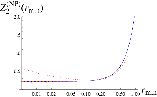
Using these results we now have an explicit expression for the exact sum rule of order two of a circular annulus with Neumann bc at the borders. In particular, for $r_{min}\rightarrow 0$ one has

\displaystyle Z_{2}^{(NP)}(r_{min})\approx\frac{5\pi^{2}}{48}-\frac{155}{192}+\frac{139r_{min}^{2}}{96}+\dots

(80)

where no logarithmic divergence is present. In Fig.1 we compare the results of the present paper with the result of Ref.[2]. Notice that the effect of the zero mode is important for $r_{min}\rightarrow 0$ , where it cancels a divergent behavior, but completely negligible for $r_{min}\rightarrow 1$ .

Incidentally we have calculated numerically the sum rule of order two for a unit circle with Neumann boundary conditions at its border, obtaining the first $2000$ eigenvalues with an accuracy of 10 digits and estimating the contribution of the higher modes with Weyl’s law.

We have found

\displaystyle\left.Z_{2}^{(N)}\right|_{circle}\approx 0.2207921258

(81)

which should be compared with

\displaystyle Z_{2}^{(NP)}(0)=\frac{5\pi^{2}}{48}-\frac{155}{192}\approx 0.2207921251

(82)

It is reasonable to conjecture that $\left.Z_{2}^{(N)}\right|_{circle}=\frac{5\pi^{2}}{48}-\frac{155}{192}$ .

Refer to caption — Figure 1: Sum rule of order two for circular annulus with internal radius $r_{min}$ (and external radius $r_{max}=1$ ). The solid blue line is the exact sum rule calculated in the present paper; the dotted red line is the result of Ref.[2], which does not include the contributions of the zero mode; the dashed orange line is the asymptotic behavior of Eq.(80). The crosses are the precise numerical values obtained calculating a large number of eigenvalues numerically.

3 Conclusions

We have found out that the formulas for the sum rules involving eigenvalues of inhomogeneous systems that we have recently derived in Refs.[1, 2] are incomplete when the system has a zero mode. In one dimension this affects problems with Neumann or periodic bc, while the cases of Dirichlet or mixed Dirichlet-Neumann bc are unaffected.

In this paper we have derived the formalism which allows one to calculate the sum rules for systems containing a zero mode exactly, by considering a nonsingular problem where the negative Laplacian is shifted infinitesimally and by then properly handling the contributions of the zero mode which are finite when the shift vanishes. Our previous approach, which used a Green’s function that did not contain the zero mode, did not account for these finite contributions. We have explicitly obtained the formulas for the sum rules of order one and two; the calculation of the higher order sum rules can be performed analogously and it also involves the calculation of higher order terms in the perturbative expansion of $E_{0}$ .

The formulas derived in this paper are compared with precise numerical results obtained for an exactly solvable problem, providing a useful numerical test.

Appendix A Perturbative calculation of $E_{0}$

We describe here a perturbative approach to the calculation of the eigenvalue and eigenfunction of the lowest mode of Eq. (6).

Assuming $|\gamma|\ll 1$ we write

	$\displaystyle E_{0}$	$\displaystyle=$	$\displaystyle\sum_{n=0}^{\infty}E_{0}^{(n)}\gamma^{n}$		(83)
	$\displaystyle\Psi_{0}(x_{1},\dots,x_{d})$	$\displaystyle=$	$\displaystyle\sum_{n=0}^{\infty}\Psi_{0}^{(n)}(x_{1},\dots,x_{d})\gamma^{n}$

Let us call $\left\{\phi_{n}(x_{1},\dots,x_{d})\right\}$ the basis obeying the boundary conditions of the problem; it is easy to see that

	$\displaystyle E_{0}^{(0)}$	$\displaystyle=$	$\displaystyle 0$		(84)
	$\displaystyle\Psi_{0}^{(0)}(x_{1},\dots,x_{d})$	$\displaystyle=$	$\displaystyle\phi_{0}(x_{1},\dots,x_{d})=\frac{1}{\sqrt{V_{\Omega}}}$		(85)

To first order one obtains the equation

\displaystyle(-\Delta)\Psi_{0}^{(1)}(x_{1},\dots,x_{d})+\Psi_{0}^{(0)}(x_{1},\dots,x_{d})=E_{0}^{(1)}\Sigma(x_{1},\dots,x_{d})\Psi_{0}^{(0)}(x_{1},\dots,x_{d})

(86)

which can be solved requiring

$\displaystyle E_{0}^{(1)}$	$\displaystyle=$	$\displaystyle\frac{V_{\Omega}}{\int_{\Omega_{d}}d^{d}x\Sigma(x_{1},\dots,x_{d})}$	(87)
$\displaystyle\Psi_{0}^{(1)}(x_{1},\dots,x_{d})$	$\displaystyle=$	$\displaystyle\sum_{m}^{\prime}c_{m}^{(1)}\phi_{m}(x_{1},\dots,x_{d})$
	$\displaystyle=$	$\displaystyle\frac{E_{0}^{(1)}}{\sqrt{V_{\Omega}}}\sum_{m}^{\prime}\frac{\int_{\Omega_{d}}d^{d}y\Sigma(y_{1},\dots,y_{d})\phi_{m}(y_{1},\dots,y_{d})}{\epsilon_{m}}\phi_{m}(x_{1},\dots,x_{d})$
	$\displaystyle=$	$\displaystyle\frac{E_{0}^{(1)}}{\sqrt{V_{\Omega}}}\int_{\Omega_{d}}d^{d}y\ G^{(0)}(x_{1},\dots,x_{d};y_{1},\dots,y_{d})\Sigma(y_{1},\dots,y_{d})$

To second order one obtains the equation

\displaystyle(-\Delta)\Psi_{0}^{(2)}(x_{1},\dots,x_{d})+\Psi_{0}^{(1)}(x_{1},\dots,x_{d})=\Sigma(x_{1},\dots,x_{d})\left(E_{0}^{(2)}\Psi_{0}^{(0)}(x_{1},\dots,x_{d})+E_{0}^{(1)}\Psi_{0}^{(1)}(x_{1},\dots,x_{d})\right)

In this case we have

$\displaystyle E_{0}^{(2)}$	$\displaystyle=$	$\displaystyle-E_{0}^{(1)}\sqrt{V_{\Omega}}\frac{\int_{\Omega}d^{d}x\ \Sigma(x_{1},\dots,x_{d})\Psi_{0}^{(1)}(x_{1},\dots,x_{d})}{\int_{\Omega}d^{d}x\Sigma(x_{1},\dots,x_{d})}$
	$\displaystyle=$	$\displaystyle-\frac{\left(E_{0}^{(1)}\right)^{2}}{\int_{\Omega}d^{d}x\ \Sigma(x_{1},\dots,x_{d})}\sum_{m}^{\prime}\frac{\left(\int_{\Omega}d^{d}x\Sigma(x_{1},\dots,x_{d})\ \phi_{m}(x_{1},\dots,x_{d})\right)^{2}}{\epsilon_{m}}$
	$\displaystyle=$	$\displaystyle-\left(E_{0}^{(1)}\right)^{2}\frac{\int_{\Omega}d^{d}x\ \int_{\Omega}d^{d}y\ \Sigma(x_{1},\dots,x_{d})\ G^{(0)}(x_{1},\dots,x_{d};y_{1},\dots,y_{d})\ \Sigma(y_{1},\dots,y_{d})}{\int_{\Omega}d^{d}x\ \Sigma(x_{1},\dots,x_{d})}$
$\displaystyle\Psi_{0}^{(2)}(x_{1},\dots,x_{d})$	$\displaystyle=$	$\displaystyle\sum_{m\neq 0}c_{m}^{(2)}\phi_{m}(x_{1},\dots,x_{d})$
	$\displaystyle=$	$\displaystyle\frac{E_{0}^{(2)}}{\sqrt{V_{\Omega}}}\sum_{m\neq 0}\frac{1}{\epsilon_{m}}\int_{\Omega_{d}}d^{d}y\ \Sigma(y_{1},\dots,y_{d})\phi_{m}(y_{1},\dots,y_{d})\phi_{m}(x_{1},\dots,x_{d})$
	$\displaystyle+$	$\displaystyle E_{0}^{(1)}\sum_{m\neq 0}\frac{1}{\epsilon_{m}}\int_{\Omega_{d}}d^{d}y\ \Sigma(y_{1},\dots,y_{d})\Psi_{0}^{(1)}(y_{1},\dots,y_{d})\phi_{m}(y_{1},\dots,y_{d})\phi_{m}(x_{1},\dots,x_{d})$
	$\displaystyle-$	$\displaystyle\frac{E_{0}^{(1)}}{\sqrt{V_{\Omega}}}\sum_{m\neq 0}\frac{\int_{\Omega_{d}}d^{d}y\Sigma(y_{1},\dots,y_{d})\phi_{m}(y_{1},\dots,y_{d})}{\epsilon_{m}^{2}}\phi_{m}(x_{1},\dots,x_{d})$
	$\displaystyle=$	$\displaystyle\frac{E_{0}^{(2)}}{\sqrt{V_{\Omega}}}\int_{\Omega_{d}}d^{d}y\ G^{(0)}(x_{1},\dots,x_{d};y_{1},\dots,y_{d})\ \Sigma(y_{1},\dots,y_{d})$
	$\displaystyle+$	$\displaystyle E_{0}^{(1)}\int_{\Omega_{d}}d^{d}y\ G^{(0)}(x_{1},\dots,x_{d};y_{1},\dots,y_{d})\Sigma(y_{1},\dots,y_{d})\Psi_{0}^{(1)}(y_{1},\dots,y_{d})$
	$\displaystyle-$	$\displaystyle\frac{E_{0}^{(1)}}{\sqrt{V_{\Omega}}}\int_{\Omega_{d}}d^{d}y\ G^{(1)}(x_{1},\dots,x_{d};y_{1},\dots,y_{d})\ \Sigma(y_{1},\dots,y_{d})$

To third order one obtains the equation

\displaystyle(-\Delta)\Psi_{0}^{(3)}(x_{1},\dots,x_{d})+\Psi_{0}^{(2)}(x_{1},\dots,x_{d})=\Sigma(x_{1},\dots,x_{d})\ \sum_{k=1}^{3}E_{0}^{(k)}\Psi_{0}^{(3-k)}(x_{1},\dots,x_{d})

In this case we have

$\displaystyle E_{0}^{(3)}$	$\displaystyle=$	$\displaystyle-E_{0}^{(2)}\sqrt{V_{\Omega}}\frac{\int_{\Omega}d^{d}x\ \Sigma(x_{1},\dots,x_{d})\Psi_{0}^{(1)}(x_{1},\dots,x_{d})}{\int_{\Omega}d^{d}x\Sigma(x_{1},\dots,x_{d})}$
	$\displaystyle-$	$\displaystyle E_{0}^{(1)}\sqrt{V_{\Omega}}\frac{\int_{\Omega}d^{d}x\ \Sigma(x_{1},\dots,x_{d})\Psi_{0}^{(2)}(x_{1},\dots,x_{d})}{\int_{\Omega}d^{d}x\Sigma(x_{1},\dots,x_{d})}$
	$\displaystyle=$	$\displaystyle-\frac{2E_{0}^{(2)}E_{0}^{(1)}}{\int_{\Omega}d^{d}x\Sigma(x_{1},\dots,x_{d})}\sum_{m}^{\prime}\frac{\left(\int_{\Omega}d^{d}x\Sigma(x_{1},\dots,x_{d})\ \phi_{m}(x_{1},\dots,x_{d})\right)^{2}}{\epsilon_{m}}$
	$\displaystyle-$	$\displaystyle\frac{\left(E_{0}^{(1)}\right)^{3}}{\int_{\Omega}d^{d}x\Sigma(x_{1},\dots,x_{d})}\sum_{n}^{\prime}\sum_{m}^{\prime}\frac{\left(\int_{\Omega}d^{d}x\Sigma(x)\ \phi_{m}(x)\right)\left(\int_{\Omega}d^{d}x\phi_{n}(x)\Sigma(x)\ \phi_{m}(x)\right)\left(\int_{\Omega}d^{d}x\Sigma(x)\ \phi_{n}(x)\right)}{\epsilon_{m}\epsilon_{n}}$
	$\displaystyle+$	$\displaystyle\frac{\left(E_{0}^{(1)}\right)^{2}}{\int_{\Omega}d^{d}x\Sigma(x_{1},\dots,x_{d})}\sum_{m}^{\prime}\frac{\left(\int_{\Omega}d^{d}x\Sigma(x)\ \phi_{m}(x)\right)^{2}}{\epsilon_{m}^{2}}$

Notice that the expressions above can be conveniently expressed in terms of the matrix elements

\displaystyle\langle m|\Sigma|n\rangle\equiv\int_{\Omega}d^{d}x\phi_{n}(x)\Sigma(x)\ \phi_{m}(x)

where

\displaystyle\langle 0|\Sigma|n\rangle\equiv\frac{1}{\sqrt{V_{\Omega}}}\int_{\Omega}d^{d}x\Sigma(x)\ \phi_{m}(x)

$\displaystyle E_{0}^{(2)}$	$\displaystyle=$	$\displaystyle-\frac{V_{\Omega}\left(E_{0}^{(1)}\right)^{2}}{\int_{\Omega}d^{d}x\ \Sigma(x_{1},\dots,x_{d})}\sum_{m}^{\prime}\frac{\langle 0\|\Sigma\|m\rangle\langle m\|\Sigma\|0\rangle}{\epsilon_{m}}$
$\displaystyle E_{0}^{(3)}$	$\displaystyle=$	$\displaystyle-\frac{2V_{\Omega}E_{0}^{(2)}E_{0}^{(1)}}{\int_{\Omega}d^{d}x\Sigma(x_{1},\dots,x_{d})}\sum_{m}^{\prime}\frac{\langle 0\|\Sigma\|m\rangle\langle m\|\Sigma\|0\rangle}{\epsilon_{m}}$
	$\displaystyle-$	$\displaystyle\frac{V_{\Omega}\left(E_{0}^{(1)}\right)^{3}}{\int_{\Omega}d^{d}x\Sigma(x_{1},\dots,x_{d})}\sum_{n}^{\prime}\sum_{m}^{\prime}\frac{\langle 0\|\Sigma\|m\rangle\langle m\|\Sigma\|n\rangle\langle n\|\Sigma\|0\rangle}{\epsilon_{m}\epsilon_{n}}$
	$\displaystyle+$	$\displaystyle\frac{V_{\Omega}\left(E_{0}^{(1)}\right)^{2}}{\int_{\Omega}d^{d}x\Sigma(x_{1},\dots,x_{d})}\sum_{m}^{\prime}\frac{\langle 0\|\Sigma\|m\rangle\langle m\|\Sigma\|0\rangle}{\epsilon_{m}^{2}}$

Acknowledgments

This research was supported by the Sistema Nacional de Investigadores (México).

References

[1] P. Amore, "Exact sum rules for inhomogeneous strings", in press, Annals of Physics (2013)
[2] P. Amore, Annals of Physics 336, 223-244 (2013)
[3] H. P. W. Gottlieb, Journal of Sound and Vibration 135, 79-83 (1989)
[4] E. Merzbacher, Quantum mechanics. Second Ed. New York. Wiley. pag.429-430

Exact sum rules for inhomogeneous systems containing a zero mode

Abstract

Keywords:

1 Introduction

2 Applications

2.1 Isospectral strings

2.2 A string with rapidly oscillating density

2.3 Circular annulus

3 Conclusions

Appendix A Perturbative calculation of E0E_{0}

Acknowledgments

References

Appendix A Perturbative calculation of $E_{0}$