跳到论文正文
W Papers独立论文阅读器 arXiv:1310.5396 论文正文 计算阅读时间 · 0%
引用这篇论文根据当前论文元数据生成,正式投稿前建议核对。


License: arXiv.org perpetual non-exclusive license
arXiv:1310.5396v2 [math.CO] 21 Nov 2014

On the local profiles of trees

Sébastien Bubeck Note: Department of Operations Research and Financial Engineering, Princeton University, Princeton 08540, USA. Email: sbubeck@princeton.edu.    Nati Linial ††thanks: Research supported in part by grants from the ISF and I-Core. Note: School of Computer Science and Engineering, The Hebrew University of Jerusalem, Jerusalem 91904, Israel. Email: nati@cs.huji.ac.il.
Abstract

We study the local profiles of trees. We show that, in contrast with the situation for general graphs, the limit set of kk-profiles of trees is convex. We initiate a study of the defining inequalities of this convex set. Many challenging problems remain open.

1 Introduction

For (unlabelled) trees TT, SS, we denote by c⁡(S,T)c(S,T) the number of copies of SS in TT, or in other words the number of injective homomorphism from SS to TT. Let T1k,…,TNkkT_{1}^{k},\ldots,T_{N_{k}}^{k} be a list of all (isomorphism types of) kk-vertex trees11 1 Recall that the sequence (Nk)k≥1(N_{k})_{k\geq 1} starts with 1,1,1,2,3,6​…1,1,1,2,3,6\ldots., where T1k,T2kT_{1}^{k},T_{2}^{k} are the kk-vertex path and the kk-vertex star, respectively. The kk-profile of a tree TT is the vector p(k)​(T)∈ℝNkp^{(k)}(T)\in\mathbb{R}^{N_{k}} whose ii-th coordinate is

(p(k)​(T))i=c⁡(Tik,T)Zk​(T),where​Zk​(T)=∑j=1Nkc⁡(Tjk,T).(p^{(k)}(T))_{i}=\frac{c(T^{k}_{i},T)}{Z_{k}(T)},\ \text{where}\ Z_{k}(T)=\sum_{j=1}^{N_{k}}c(T^{k}_{j},T).

In other words the kk-profile is the induced density vector of kk-vertex trees. We are interested in understanding the limit set of kk-profiles:

Δ𝒯(k)={p∈ℝNk:∃(Tn),|Tn|→n→∞∞,andp(k)(Tn)→n→∞p},\Delta_{\mathcal{T}}(k)=\left\{p\in\mathbb{R}^{N_{k}}:\exists(T_{n}),|T_{n}|\xrightarrow[n\rightarrow\infty]{}\infty,\,\text{and}\,p^{(k)}(T_{n})\xrightarrow[n\rightarrow\infty]{}p\right\},

where |T||T| denotes the number of vertices in TT. Our main result, proved in Section 2, is:

Theorem 1

The set Δ𝒯​(k)\Delta_{\mathcal{T}}(k) is convex.

This property of profiles of trees is in sharp contrast with what happens for general graphs. Let Δ⁡(k)\Delta(k) be the kk-profiles limit set of general graphs (which is defined like Δ𝒯​(k)\Delta_{\mathcal{T}}(k) with a list of all kk-vertex graphs rather than kk-vertex trees). The first and second coordinates in p∈Δ⁡(k)p\in\Delta(k) correspond to kk-anticliques and kk-cliques respectively. Clearly e1=(1,0,…,0),e2=(0,1,0,…,0)∈Δ⁡(k)e_{1}=(1,0,\ldots,0),e_{2}=(0,1,0,\ldots,0)\in\Delta(k) but 12​e1+12​e2∉Δ⁡(k)\frac{1}{2}e_{1}+\frac{1}{2}e_{2}\not\in\Delta(k). Not only is Δ⁡(k)\Delta(k) nonconvex, it is even computationally infeasible to derive a description of its convex hull, see Hatami and Norine (2011). Our understanding of the sets Δ⁡(k)\Delta(k) is rather fragmentary (e.g. Huang et al. (2012)). Flag algebras Razborov (2007) are a major tool in such investigations. The convexity of Δ𝒯​(k)\Delta_{\mathcal{T}}(k) suggests that we may have a better chance understanding profiles of trees, by deriving the linear inequalities that define these sets. We take some steps in this direction. Concretely we prove the following result in Section 3.

Theorem 2

Let p∈Δ𝒯​(k)p\in\Delta_{\mathcal{T}}(k), then

p1+p2≥12​Nk​k2​k.p_{1}+p_{2}\geq\frac{1}{2N_{k}k^{2k}}.

We suspect that a stronger lower bound holds here. In Section 3 we give examples which show that p1+p2p_{1}+p_{2} can be exponentially small in kk.

For 55-profiles we get a better inequality. In Section 4 we prove

Theorem 3

Let p∈Δ𝒯​(5)p\in\Delta_{\mathcal{T}}(5), then

p2≥1−2​p137.p_{2}\geq\frac{1-2p_{1}}{37}.

The above inequality holds with equality at the point (1/2,0)∈Δ𝒯​(5)(1/2,0)\in\Delta_{\mathcal{T}}(5), but we believe that it is not tight for p∈Δ𝒯​(5)p\in\Delta_{\mathcal{T}}(5) such that p2>0p_{2}>0. We discuss tightness in more detail in Section 4. We end the paper with a list of open problems in Section 5.

2 Convexity of the kk-profiles limit set

In this Section we prove Theorem 1. We first explain how to “glue” two trees, and then we show how gluing allows us to generate convex combinations of tree profiles.

Step 1: the gluing operation. If TT and SS are trees, we define T⊠kST\boxtimes_{k}S as follows. This is a tree which consists of a copy of TT, a copy of SS and a (k−1)(k-1)-vertex path that connects some arbitrary leaf xx in TT to an arbitrary leaf yy in SS. In other words, we add to SS and TT a path x=z0,…,zk=yx=z_{0},\ldots,z_{k}=y where z1,…,zk−1z_{1},\ldots,z_{k-1} are new vertices. The resulting tree depends of course on the choice of the two leaves xx and yy, but we ignore this issue, since this will not affect anything that is said below.

We denote by D⁡(K)D(K) the largest vertex degree in a given tree KK. The following inequalities are easy to verify:

c⁡(Tik,T)+c⁡(Tik,S)≤c⁡(Tik,T⊠kS)≤c⁡(Tik,T)+c⁡(Tik,S)+k​D​(T)k−2+k​D​(S)k−2,\displaystyle c(T^{k}_{i},T)+c(T^{k}_{i},S)\leq c(T^{k}_{i},T\boxtimes_{k}S)\leq c(T^{k}_{i},T)+c(T^{k}_{i},S)+kD(T)^{k-2}+kD(S)^{k-2}, (1)

and consequently

Zk​(T)+Zk​(S)≤Zk​(T⊠kS)≤Zk​(T)+Zk​(S)+k​Nk​D​(T)k−2+k​Nk​D​(S)k−2.\displaystyle Z_{k}(T)+Z_{k}(S)\leq Z_{k}(T\boxtimes_{k}S)\leq Z_{k}(T)+Z_{k}(S)+kN_{k}D(T)^{k-2}+kN_{k}D(S)^{k-2}. (2)

We define by induction T⊠kℓ=T⊠k(ℓ−1)⊠kTT^{\boxtimes_{k}\ell}=T^{\boxtimes_{k}(\ell-1)}\boxtimes_{k}T (with T⊠k1=TT^{\boxtimes_{k}1}=T). Observe that D(T⊠kℓ)=D(T)D(T^{\boxtimes_{k}\ell})=D(T) and thus using (1) and (2) one has

ℓc(Tik,T)≤c(Tik,T⊠kℓ)≤ℓc(Tik,T)+2k(ℓ−1)D(T)k−2,\displaystyle\ell c(T^{k}_{i},T)\leq c(T^{k}_{i},T^{\boxtimes_{k}\ell})\leq\ell c(T^{k}_{i},T)+2k(\ell-1)D(T)^{k-2}, (3)
ℓZk(T)≤Zk(T⊠kℓ)≤ℓZk(T)+2kNk(ℓ−1)D(T)k−2.\displaystyle\ell Z_{k}(T)\leq Z_{k}(T^{\boxtimes_{k}\ell})\leq\ell Z_{k}(T)+2kN_{k}(\ell-1)D(T)^{k-2}. (4)

Step 2: convex combinations by gluing. Let p,q∈Δ𝒯​(k)p,q\in\Delta_{\mathcal{T}}(k). Namely, there exists two sequences of trees TnT_{n} and SnS_{n} such that

|Tn|,|Sn|→n→∞∞,and​(p(k)​(Tn),p(k)​(Sn))→n→∞(p,q).|T_{n}|,|S_{n}|\xrightarrow[n\rightarrow\infty]{}\infty,\,\text{and}\,(p^{(k)}(T_{n}),p^{(k)}(S_{n}))\xrightarrow[n\rightarrow\infty]{}(p,q).

Now, given λ∈(0,1)\lambda\in(0,1), we want to construct a sequence of trees RnR_{n} such that

|Rn|→n→∞∞,and​p(k)​(Rn)→n→∞λ​p+(1−λ)​q.|R_{n}|\xrightarrow[n\rightarrow\infty]{}\infty,\,\text{and}\,p^{(k)}(R_{n})\xrightarrow[n\rightarrow\infty]{}\lambda p+(1-\lambda)q.

First let αn/βn\alpha_{n}/\beta_{n} be a sequence of rational numbers that converges to λ\lambda. We correspondingly define the sequence of trees RnR_{n} via:

Rn=Tn⊠k[αnZk(Sn)]⊠kSn⊠k[(βn−αn)Zk(Tn)].R_{n}=T_{n}^{\boxtimes_{k}[\alpha_{n}Z_{k}(S_{n})]}\boxtimes_{k}S_{n}^{\boxtimes_{k}[(\beta_{n}-\alpha_{n})Z_{k}(T_{n})]}.

Using (2) and (4) one immediately obtains

βn​Zk​(Tn)​Zk​(Sn)\displaystyle\beta_{n}Z_{k}(T_{n})Z_{k}(S_{n})
≤Zk​(Rn)\displaystyle\leq Z_{k}(R_{n}) (5)
≤βn​Zk​(Tn)​Zk​(Sn)+2​k​Nk​αn​Zk​(Sn)​D​(Tn)k−2+2​k​Nk​(βn−αn)​Zk​(Tn)​D​(Sn)k−2.\displaystyle\leq\beta_{n}Z_{k}(T_{n})Z_{k}(S_{n})+2kN_{k}\alpha_{n}Z_{k}(S_{n})D(T_{n})^{k-2}+2kN_{k}(\beta_{n}-\alpha_{n})Z_{k}(T_{n})D(S_{n})^{k-2}.

Now the key observation is that

D​(Tn)k−2=o⁡(Zk​(Tn)).D(T_{n})^{k-2}=o(Z_{k}(T_{n})). (6)

Indeed, Zk​(Tn)≥(D⁡(Tn)k−1)Z_{k}(T_{n})\geq{D(T_{n})\choose k-1} follows by counting kk-vertex stars rooted at the highest degree vertex in TnT_{n}, which yields equation (6) if D⁡(Tn)→∞D(T_{n})\to\infty. On the other hand, if D⁡(Tn)D(T_{n}) is bounded then (6) is also clearly true since Zk​(Tn)→∞Z_{k}(T_{n})\to\infty.

Using (6) one can rewrite (5) as

Zk​(Rn)=βn​Zk​(Tn)​Zk​(Sn)+o⁡(βn​Zk​(Tn)​Zk​(Sn)).Z_{k}(R_{n})=\beta_{n}Z_{k}(T_{n})Z_{k}(S_{n})+o(\beta_{n}Z_{k}(T_{n})Z_{k}(S_{n})).

Similarly using (1) and (3) we obtain

c⁡(Tik,Rn)=αn​Zk​(Sn)​c​(Tik,Tn)+(βn−αn)​Zk​(Tn)​c​(Tik,Sn)+o⁡(βn​Zk​(Tn)​Zk​(Sn)).c(T_{i}^{k},R_{n})=\alpha_{n}Z_{k}(S_{n})c(T_{i}^{k},T_{n})+(\beta_{n}-\alpha_{n})Z_{k}(T_{n})c(T_{i}^{k},S_{n})+o(\beta_{n}Z_{k}(T_{n})Z_{k}(S_{n})).

We combine these two identities and conclude that

(p(k)​(Rn))i=c⁡(Tik,Rn)Zk​(Rn)=(1+o⁡(1))​[αnβn​c⁡(Tik,Tn)Zk​(Tn)+(1−αnβn)​c⁡(Tik,Sn)Zk​(Sn)]+o⁡(1)→λ​pi+(1−λ)​qi,(p^{(k)}(R_{n}))_{i}=\frac{c(T_{i}^{k},R_{n})}{Z_{k}(R_{n})}=(1+o(1))\left[\frac{\alpha_{n}}{\beta_{n}}\frac{c(T_{i}^{k},T_{n})}{Z_{k}(T_{n})}+\left(1-\frac{\alpha_{n}}{\beta_{n}}\right)\frac{c(T_{i}^{k},S_{n})}{Z_{k}(S_{n})}\right]+o(1)\to\lambda p_{i}+(1-\lambda)q_{i},

as claimed.

3 On Stars and Paths

In this Section we prove Theorem 2. We use the shorthand Pk​(T)=c⁡(T1k,T)P_{k}(T)=c(T^{k}_{1},T) and Sk​(T)=c⁡(T2k,T)S_{k}(T)=c(T^{k}_{2},T), and we also omit the reference to TT whenever it is clear from context. Before delving into the proof let us show why the exponential decrease in kk is unavoidable. A dd-millipede is a tree where all non-leaf vertices reside on a single path and they have degree d+2d+2 each. See Figure 1 for an illustration. The number of non-leaves is called the dd-millipede’s length.

dd
Figure 1: A dd-millipede.

We denote by TnT_{n} the (k−4)(k-4)-millipede of length nn with kk even. Also, RkR_{k} is the k−42\frac{k-4}{2}-millipede of length 22. It is easy to see that for k≥6k\geq 6,

Zk​(Tn)≥c⁡(Rk,Tn)≥2​(n−2)​(k−3(k−2)/2)≥(n−2)​(3/2)k/2,Z_{k}(T_{n})\geq c(R_{k},T_{n})\geq 2(n-2){k-3\choose(k-2)/2}\geq(n-2)(3/2)^{k/2},

and

Sk​(Tn)=0,Pk​(Tn)≤n​(k−3)2.S_{k}(T_{n})=0,\qquad P_{k}(T_{n})\leq n(k-3)^{2}.

Thus the limiting profile that corresponds to the sequence (Tn)(T_{n}) satisfies

p1+p2≤(k−3)2(3/2)k/2.p_{1}+p_{2}\leq\frac{(k-3)^{2}}{(3/2)^{k/2}}. (7)

For k>3k>3, let 𝒫⁡(k)\mathcal{P}(k) be the projection of Δ⁡(k)\Delta(k) on the first two coordinates, that is

𝒫⁡(k)={(p1,p2),p∈Δ𝒯​(k)}.\mathcal{P}(k)=\{(p_{1},p_{2}),p\in\Delta_{\mathcal{T}}(k)\}.

As a side note we also observe that the above inequality yields:

∪k𝒫(k)¯={x∈ℝ+2:x1+x2≤1},\overline{{\cup_{k}\mathcal{P}(k)}}=\{x\in\mathbb{R}_{+}^{2}:x_{1}+x_{2}\leq 1\},

where A¯\overline{A} denotes the closure of a set AA. Indeed (1,0)(1,0) and (0,1)(0,1) are always in 𝒫⁡(k)\mathcal{P}(k), (7) shows that for kk large enough one can find a point arbitrarily close to (0,0)(0,0), and thus using the convexity of 𝒫⁡(k)\mathcal{P}(k) (Theorem 1) one obtains the above set equality.

We now turn to the proof of Theorem 2. We repeatedly use the following obvious result which we state without a proof.

Lemma 1

A tree with maximal degree DD has at most k​Nk​Dk−1kN_{k}D^{k-1} kk-vertex subtrees that contain a given vertex.

Lemma 2 is an enumerative analog of the probabilistic statement of Theorem 2 which applies when Sk=0S_{k}=0. In Lemma 3 we deal with the case of Sk≥0S_{k}\geq 0, which then yields Theorem 2.

Lemma 2

If D⁡(T)≤k−2D(T)\leq k-2 for some tree TT, then

Zk≤k​Nk​(k−2)k−1​Pk+k​Nk​(k−2)2​k−2.Z_{k}\leq kN_{k}(k-2)^{k-1}P_{k}+kN_{k}(k-2)^{2k-2}.

Proof For trees with n≤(k−2)k−1n\leq(k-2)^{k-1} vertices this inequality clearly follows from Lemma 1. For n>(k−2)k−1n>(k-2)^{k-1} we proceed by induction. Clearly for this range of nn, the tree’s diameter must be at least 2​(k−2)2(k-2). In other words it must contain a copy PP of P2​(k−2)+1P_{2(k-2)+1}. Let the tree T′T^{\prime} be obtained by removing a leaf xx from TT. This eliminates at least one kk-vertex path, namely the path from xx toward PP possibly proceeding toward PP’s furthest end. In other words:

Pk​(T)≥Pk​(T′)+1.P_{k}(T)\geq P_{k}(T^{\prime})+1.

Furthermore by Lemma 1

Zk​(T)≤Zk​(T′)+k​Nk​(k−2)k−1.Z_{k}(T)\leq Z_{k}(T^{\prime})+kN_{k}(k-2)^{k-1}.

Applying the induction hypothesis to T′T^{\prime} yields

Zk​(T′)≤k​Nk​(k−2)k−1​Pk​(T′)+k​Nk​(k−2)2​k−2,Z_{k}(T^{\prime})\leq kN_{k}(k-2)^{k-1}P_{k}(T^{\prime})+kN_{k}(k-2)^{2k-2},

together with the two above inequalities this gives the same inequality for TT.  

Lemma 3

Every tree satisfies

Zk≤Nk​k2​k​(Pk+2​Sk+1).Z_{k}\leq N_{k}k^{2k}(P_{k}+2S_{k}+1).

Proof First observe that if n≤kkn\leq k^{k} then by (a variant of) Lemma 1:

Zk\displaystyle Z_{k} ≤\displaystyle\leq ∑u:d⁡(u)≤k−2kNkd(u)k−1+∑u:d⁡(u)≥k−1kNkd(u)k−1\displaystyle\sum_{u:d(u)\leq k-2}kN_{k}d(u)^{k-1}+\sum_{u:d(u)\geq k-1}kN_{k}d(u)^{k-1}
≤\displaystyle\leq Nkk2​k+∑u:d⁡(u)≥k−1kNk(k−1)k−1(d⁡(u)k−1)\displaystyle N_{k}k^{2k}+\sum_{u:d(u)\geq k-1}kN_{k}(k-1)^{k-1}{d(u)\choose k-1}
≤\displaystyle\leq Nk​k2​k+Nk​kk​Sk,\displaystyle N_{k}k^{2k}+N_{k}k^{k}S_{k},

as needed. For larger trees we prove the following stronger inequality by induction on the number of vertices:

Zk≤Nkk2​k(Pk+1)𝟙{Pk≥1}+2Nkk2​kSk.Z_{k}\leq N_{k}k^{2k}\left(P_{k}+1\right)\mathds{1}\{P_{k}\geq 1\}+2N_{k}k^{2k}S_{k}.

Clearly the expression 𝟙{Pk≥1}\mathds{1}\{P_{k}\geq 1\} captures the information whether or not TT’s diameter is at least k−1k-1. The base case n=kkn=k^{k} follows since necessarily Pk≥1P_{k}\geq 1 or Sk≥1S_{k}\geq 1. The induction step has two cases:

Case 1: If D⁡(T)≤k−2D(T)\leq k-2, then Lemma 2 yields the inequality, since Pk≥1P_{k}\geq 1.

Case 2: Let vv be the vertex of largest degree d≥k−1d\geq k-1, and let T1,…,TdT_{1},\ldots,T_{d} be the trees of the forest T∖{v}T\setminus\{v\}. By Lemma 1

Zk​(T)≤∑i=1dZk​(Ti)+k​Nk​dk−1.Z_{k}(T)\leq\sum_{i=1}^{d}Z_{k}(T_{i})+kN_{k}d^{k-1}.

Furthermore

Sk​(T)≥∑i=1dSk​(Ti)+(dk−1)≥∑i=1dSk​(Ti)+(dk−1)k−1,S_{k}(T)\geq\sum_{i=1}^{d}S_{k}(T_{i})+{d\choose k-1}\geq\sum_{i=1}^{d}S_{k}(T_{i})+\left(\frac{d}{k-1}\right)^{k-1},

and

(1+Pk(T))𝟙{Pk(T)≥1}≥∑i=1d(1+Pk(Ti))𝟙{Pk(Ti)≥1}.(1+P_{k}(T))\mathds{1}\{P_{k}(T)\geq 1\}\geq\sum_{i=1}^{d}(1+P_{k}(T_{i}))\mathds{1}\{P_{k}(T_{i})\geq 1\}.

To see why the last inequality holds true, observe first that it is trivial if ∑i=1d𝟙{Pk(Ti)≥1}∈{0,1}\sum_{i=1}^{d}\mathds{1}\{P_{k}(T_{i})\geq 1\}\in\{0,1\}. Furthermore if ∑i=1d𝟙{Pk(Ti)≥1}≥2\sum_{i=1}^{d}\mathds{1}\{P_{k}(T_{i})\geq 1\}\geq 2, then for each ii such that Pk​(Ti)≥1P_{k}(T_{i})\geq 1, one can find a path in TT containing both vv and vertices from TiT_{i}, which means that in this case one even has Pk(T)≥∑i=1d(1+Pk(Ti))𝟙{Pk(Ti)≥1}P_{k}(T)\geq\sum_{i=1}^{d}(1+P_{k}(T_{i}))\mathds{1}\{P_{k}(T_{i})\geq 1\}.

Combine the three above displays and apply induction to the TiT_{i}’s to conclude:

Zk​(T)\displaystyle Z_{k}(T) ≤\displaystyle\leq ∑i=1dZk​(Ti)+k​Nk​dk−1\displaystyle\sum_{i=1}^{d}Z_{k}(T_{i})+kN_{k}d^{k-1}
≤\displaystyle\leq Nkk2​k∑i=1d(Pk(Ti)+1)𝟙{Pk(Ti)≥1}+2Nkk2​k∑i=1dSk(Ti)+kNkdk−1\displaystyle N_{k}k^{2k}\sum_{i=1}^{d}\left(P_{k}(T_{i})+1\right)\mathds{1}\{P_{k}(T_{i})\geq 1\}+2N_{k}k^{2k}\sum_{i=1}^{d}S_{k}(T_{i})+kN_{k}d^{k-1}
≤\displaystyle\leq Nkk2​k(1+Pk(T))𝟙{Pk(T)≥1}+2Nkk2​kSk(T),\displaystyle N_{k}k^{2k}(1+P_{k}(T))\mathds{1}\{P_{k}(T)\geq 1\}+2N_{k}k^{2k}S_{k}(T),

which concludes the proof.  

4 55-profiles

Clearly Δ⁡(5)\Delta(5) is entirely determined by 𝒫⁡(5)\mathcal{P}(5). In this Section we prove Theorem 3 which improves Theorem 2 for k=5k=5.

Before we embark on the proof we show that millipedes generate a ’large’ set of points in 𝒫⁡(5)\mathcal{P}(5). To simplify notation, let P⁡(T)=c⁡(T15,T)P(T)=c(T^{5}_{1},T), S⁡(T)=c⁡(T25,T)S(T)=c(T^{5}_{2},T) and Y⁡(T)=c⁡(T35,T)Y(T)=c(T^{5}_{3},T) (note that T35T^{5}_{3} has the YY-shape). We also omit the dependency on TT whenever it is clear from context. For a dd-millipede of length nn we get the following expressions:

S\displaystyle S =\displaystyle= n​(d+24),\displaystyle n{d+2\choose 4},
P\displaystyle P =\displaystyle= (n−2)​(d+1)2,\displaystyle(n-2)(d+1)^{2},
Y\displaystyle Y =\displaystyle= 2​(n−2)​(d+12)​(d+1)+2​(d+12)​(d+1)=(n−1)​(d+1)2​d,\displaystyle 2(n-2){d+1\choose 2}(d+1)+2{d+1\choose 2}(d+1)=(n-1)(d+1)^{2}d,
S+Y+P\displaystyle S+Y+P =\displaystyle= n​(d+24)+(n−2)​(d+1)3+(d+1)2​d.\displaystyle n{d+2\choose 4}+(n-2)(d+1)^{3}+(d+1)^{2}d.

In particular for fixed dd and n→∞n\to\infty, we get the following point in 𝒫⁡(5)\mathcal{P}(5):

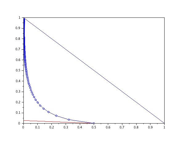
md=((d+1)2(d+24)+(d+1)3,(d+24)(d+24)+(d+1)3).m_{d}=\left(\frac{(d+1)^{2}}{{d+2\choose 4}+(d+1)^{3}},\frac{{d+2\choose 4}}{{d+2\choose 4}+(d+1)^{3}}\right). (8)

Thus by convexity we have

𝒫⁡(5)⊇conv⁡({(0,1)}∪{md,d≥0}).\mathcal{P}(5)\supseteq\mathrm{conv}(\{(0,1)\}\cup\{m_{d},d\geq 0\}). (9)

We cannot rule out the possibility that this is, in fact an equality. This inclusion and the inequality from Theorem 3 are illustrated in Figure 2.
Refer to caption
Figure 2: The equation of the red line is y=1−2​x37y=\frac{1-2x}{37}. In blue: the polygonal curve connecting consecutive md,d≥1m_{d},d\geq 1 of equation (8) as well as (0,1)(0,1) to (1,0)(1,0). By Theorem 3 the set 𝒫⁡(5)\mathcal{P}(5) lies above the red line and by Theorem 1 it contains the convex domain bounded by the blue lines.

Our proof of Theorem 3 proceeds along the route that we took in proving Theorem 2. Now, however, we are much more careful with the details. Lemma 4, a counterpart of Theorem 3 gives an inequality on the unnormalized quantities when S=0S=0. The general case S≥0S\geq 0 is handled in Lemma 5 which yields Theorem 3.

Lemma 4

If D⁡(T)≤3D(T)\leq 3, then

Y≤P+4,Y\leq P+4,

with equality if and only if TT is a 11-millipede.

Note that to prove Theorem 3 we will only need the inequality provided by Lemma 4.

Proof It is immediate that a 11-millipede satisfies Y=P+4Y=P+4. We prove the inequality in two steps. A third step shows that only 11-millipedes satisfy Y=P+4Y=P+4.

Step 1: a formula for P−YP-Y. We say that a vertex of degree 33 has type x​y​zxyz with x,y,z∈{0,1,2}x,y,z\in\{0,1,2\} if its three neighbors have degree x+1,y+1x+1,y+1, and z+1z+1, respectively. The number of vertices of type x​y​zxyz is denoted nx​y​zn_{xyz}. Similarly we define for degree-22 vertices the quantity nx​yn_{xy}.

A straightforward (but slightly painful) calculation yields

P=12​n222+8​n221+4​n220+5​n211+2​n210+3​n111+n110+4​n22+2​n21+n11,P=12n_{222}+8n_{221}+4n_{220}+5n_{211}+2n_{210}+3n_{111}+n_{110}+4n_{22}+2n_{21}+n_{11},

and

Y=6​n222+5​n221+4​n220+4​n211+3​n210+2​n200+3​n111+2​n110+n100.Y=6n_{222}+5n_{221}+4n_{220}+4n_{211}+3n_{210}+2n_{200}+3n_{111}+2n_{110}+n_{100}.

Hence

P−Y=6​n222+3​n221+n211−n210−2​n200−n110−n100+4​n22+2​n21+n11.P-Y=6n_{222}+3n_{221}+n_{211}-n_{210}-2n_{200}-n_{110}-n_{100}+4n_{22}+2n_{21}+n_{11}. (10)

Step 2: double counting. Let nxn_{x} be the number of degree-xx vertices. Clearly n1+n2+n3=n,n_{1}+n_{2}+n_{3}=n, and by double counting of edges, also n1+2​n2+3​n3=2​(n−1).n_{1}+2n_{2}+3n_{3}=2(n-1). In particular,

n1−n3=2.n_{1}-n_{3}=2. (11)

Next observe that n1n_{1} and n3n_{3} can easily be expressed in terms of the parameters nx​yn_{xy} and nx​y​zn_{xyz}. Namely,

n3\displaystyle n_{3} =\displaystyle= n222+n221+n220+n211+n210+n200+n111+n110+n100,\displaystyle n_{222}+n_{221}+n_{220}+n_{211}+n_{210}+n_{200}+n_{111}+n_{110}+n_{100},
n1\displaystyle n_{1} =\displaystyle= n220+n210+2​n200+n110+2​n100+n20+n10.\displaystyle n_{220}+n_{210}+2n_{200}+n_{110}+2n_{100}+n_{20}+n_{10}.

Together with (11) we find

−n222−n221−n211+n200−n111+n100+n20+n10=2.-n_{222}-n_{221}-n_{211}+n_{200}-n_{111}+n_{100}+n_{20}+n_{10}=2. (12)

Next adding (10) to twice (12) one gets

P−Y+4=4​n222+n221−n211−n210−2​n111−n110+n100+4​n22+2​n21+n11+2​n20+2​n10.P-Y+4=4n_{222}+n_{221}-n_{211}-n_{210}-2n_{111}-n_{110}+n_{100}+4n_{22}+2n_{21}+n_{11}+2n_{20}+2n_{10}.

It only remains to show that the right hand side term is non-negative. To this end we count edges between a degree-22 vertex and a degree-33 vertex in two ways: Once from the degree-33 side and once from the degree-22 side

n221+2​n211+n210+3​n111+2​n110+n100=2​n22+n21+n20.n_{221}+2n_{211}+n_{210}+3n_{111}+2n_{110}+n_{100}=2n_{22}+n_{21}+n_{20}.

This concludes the proof of the inequality stated in the theorem. Note that we have, in fact, showed a more precise statement:

P−Y+4=4​n222+2​n221+n211+n111+n110+2​n100+2​n22+n21+n11+n20+2​n10.P-Y+4=4n_{222}+2n_{221}+n_{211}+n_{111}+n_{110}+2n_{100}+2n_{22}+n_{21}+n_{11}+n_{20}+2n_{10}. (13)

Step 3: the equality case. Equation (13) shows that if P−Y+4=0P-Y+4=0 then

4​n222+2​n221+n211+n111+n110+2​n100+2​n22+n21+n11+n20+2​n10=0.4n_{222}+2n_{221}+n_{211}+n_{111}+n_{110}+2n_{100}+2n_{22}+n_{21}+n_{11}+n_{20}+2n_{10}=0.

In particular the tree contains no degree-22 vertices, and no degree-33 vertices of type 222222. In other words, it has only leaves and degree-33 vertices of types 220220 and 200200. Moreover, by (12) in this case n200=2n_{200}=2. A straightforward inductive proof shows that the tree must be a 11-millipede.  

We now adapt Lemma 4 to the case where S>0S>0. This more general inequality directly implies Theorem 3.

Lemma 5

All trees satisfy

Y≤36​S+P+4.Y\leq 36S+P+4.

Proof First observe the following expressions

Y=∑{u,v}∈E((d⁡(v)−12)⁡(d⁡(u)−1)+(d⁡(u)−12)⁡(d⁡(v)−1)).Y=\sum_{\{u,v\}\in E}\left({d(v)-1\choose 2}(d(u)-1)+{d(u)-1\choose 2}(d(v)-1)\right).

We split Y=Ys+YℓY=Y_{s}+Y_{\ell}, where

Ys=∑{u,v}∈E:max⁡(d⁡(u),d⁡(v))≤3((d⁡(v)−12)(d(u)−1)+(d⁡(u)−12)(d(v)−1)),{Y_{s}}=\sum_{\{u,v\}\in E:\max(d(u),d(v))\leq 3}\left({d(v)-1\choose 2}(d(u)-1)+{d(u)-1\choose 2}(d(v)-1)\right),

and

Yℓ=∑{u,v}∈E:max⁡(d⁡(u),d⁡(v))≥4((d⁡(v)−12)(d(u)−1)+(d⁡(u)−12)(d(v)−1)).{Y_{\ell}}=\sum_{\{u,v\}\in E:\max(d(u),d(v))\geq 4}\left({d(v)-1\choose 2}(d(u)-1)+{d(u)-1\choose 2}(d(v)-1)\right).

The proof deals separately with Ys{Y_{s}} and Yℓ{Y_{\ell}}.

Step 1: We prove that Yℓ≤36​S{Y_{\ell}}\leq 36S by observing

S=∑u∈V(d⁡(u)4)=14∑u,v:{u,v}∈E(d⁡(u)−13)=14∑{u,v}∈E((d⁡(u)−13)+(d⁡(v)−13)).S=\sum_{u\in V}{d(u)\choose 4}=\frac{1}{4}\sum_{u,v:\{u,v\}\in E}{d(u)-1\choose 3}=\frac{1}{4}\sum_{\{u,v\}\in E}\left({d(u)-1\choose 3}+{d(v)-1\choose 3}\right).

and making a term-by-term comparison with the expression for Yℓ{Y_{\ell}}. We use the fact that for any nonnegative integers x≠2,y≥3x\neq 2,y\geq 3

y​x​(x−1)+x​y​(y−1)≤x2​(x−1)+y2​(y−1)≤3​(x⁡(x−1)​(x−2)+y⁡(y−1)​(y−2)),yx(x-1)+xy(y-1)\leq x^{2}(x-1)+y^{2}(y-1)\leq 3(x(x-1)(x-2)+y(y-1)(y-2)),

and furthermore for x=2x=2 this inequality (without the intermediate step) is also true.

Step 2: We prove by induction on the size of the tree that Ys≤P+4{Y_{s}}\leq P+4. The base case is trivial. The induction step has three cases:

Case 1: D⁡(T)≤3D(T)\leq 3. The inequality follows readily from Lemma 4.

Case 2: There are two neighbors u,vu,v in TT, where d⁡(u)≥4d(u)\geq 4 and vv is a leaf. Clearly,

Ys​(T)≤Ys​(T′),and​P​(T′)≤P⁡(T){Y_{s}}(T)\leq{Y_{s}}(T^{\prime}),\ \text{and}\ P(T^{\prime})\leq P(T)

where T′:=T∖{v}T^{\prime}:=T\setminus\{v\}. By applying the induction hypothesis to T′T^{\prime} we see that Ys​(T′)≤P⁡(T′)+4{Y_{s}}(T^{\prime})\leq P(T^{\prime})+4 which implies Ys≤P+4{Y_{s}}\leq P+4.

Case 3: There is a vertex uu in TT with d⁡(u)≥4d(u)\geq 4, and no neighbor of uu is a leaf. Let vv be a neighbor of uu and let T1,T2T_{1},T_{2} be the two trees of the forest obtained by removing the edge u​vuv and adding a new edge to vv, where uu is in T1T_{1} and vv in T2T_{2}. As in Case 2

Ys​(T)≤Ys​(T1)+Ys​(T2).{Y_{s}}(T)\leq{Y_{s}}(T_{1})+{Y_{s}}(T_{2}).

Observe that we can assume that vv was selected such that T2T_{2} has at least 33 edges, for otherwise Ys​(T)=0Y_{s}(T)=0 and thus the inequality would trivially hold. Indeed if T2T_{2} had 22 edges for all neighbors of uu, then T∖{u}T\setminus\{u\} would be a matching, and thus any copy of T35T^{5}_{3} in TT would have uu in its “middle edge”, which implies Ys​(T)=0Y_{s}(T)=0.

Now clearly if T2T_{2} has at least 33 edges,

P⁡(T)≥P⁡(T1)+P⁡(T2)+2​(d⁡(u)−1)≥P⁡(T1)+P⁡(T2)+4.P(T)\geq P(T_{1})+P(T_{2})+2(d(u)-1)\geq P(T_{1})+P(T_{2})+4.

Applying the induction hypothesis to T1T_{1} and T2T_{2} and using the above inequalities yield Ys≤P+4{Y_{s}}\leq P+4 in this case as well.  

5 Open problems

  1. 1.

    Is the blue curve in Figure 2 tight? That is, is (9) in fact an equality? Less ambitiously, can the bound in Lemma 5 be improved to Y≤9​S+P+K,Y\leq 9S+P+K, for some universal K≥0K\geq 0 ? If true, this shows that the first segment of the polygonal curve is tight.

  2. 2.

    Recall that 𝒫⁡(k)\mathcal{P}(k) is the projection of the limit set of kk-profiles to the first two coordinates. Are these sets increasing, i.e., is it true that

    𝒫⁡(k)⊂𝒫⁡(k+1)\mathcal{P}(k)\subset\mathcal{P}(k+1)

    for all integer kk ?

  3. 3.

    Let p∈Δ𝒯​(k)p\in\Delta_{\mathcal{T}}(k). Does p1=0p_{1}=0 imply p2=1p_{2}=1?

  4. 4.

    Imitating a concept from graph theory we define the inducibility of a tree TT to be lim supc⁡(T,𝒯)Z|T|​(𝒯)\limsup\frac{c(T,{\cal T})}{Z_{|T|}({\cal T})} where the lim sup\limsup is over trees 𝒯{\cal T} of size tending to infinity. By gluing many copies of TT as in Section 2 it is easy to show that every TT has positive inducibility. By Theorem 2 paths and stars are the only trees with inducibility 11, but are there other trees with inducibility arbitrarily close to 11 ? If such trees do not exist, is it nonetheless possible to find infinitely many trees of inducibility ≥ε\geq\varepsilon for some ε>0\varepsilon>0 ? Note that in the realm of graphs there are infinitely many distinct graphs with inducibility >110>\frac{1}{10}, for example, the complete bipartite graphs H=K3,rH=K_{3,r} with r>10r>10. It can be easily verified that randomly chosen set of r+3r+3 vertices in K3​n,r​nK_{3n,rn} for nn large spans a copy of HH with probability >0.1>0.1.

  5. 5.

    Call a sequence of trees (Tn)(T_{n}) kk-universal if

    lim infn→∞(p(k)​(Tn))i>0\liminf_{n\rightarrow\infty}(p^{(k)}(T_{n}))_{i}>0

    for every i∈[Nk]i\in[N_{k}]. The convexity of Δ𝒯​(k)\Delta_{\mathcal{T}}(k) and the fact that every tree has positive inducibility implies that kk-universal sequences exist. But does there exist a sequence of trees which is kk-universal simultaneously for every kk ? For general graphs the answer is positive, e.g., using G⁡(n,p)G(n,p) graphs.

  6. 6.

    Is there a probabilistic interpretation to the profile of a tree?

  7. 7.

    In this paper we found only linear inequalities satisfied by the sets Δ𝒯​(k)\Delta_{\cal T}(k). We wonder if higher order inequalities can be derived as well. Is there a framework similar to flag algebras that applies to trees?

Acknowledgements

The research described here was carried out at the Simons Institute for the Theory of Computing. We are grateful to the Simons Institute for offering us such a wonderful research environment. We also thank an anonymous referee for fixing a mistake in the first version of this paper.

References

  • Hatami and Norine [2011] Hamed Hatami and Serguei Norine. Undecidability of linear inequalities in graph homomorphism densities. Journal of the American Mathematical Society, 24(2):547–565, 2011.
  • Huang et al. [2012] Hao Huang, Nati Linial, Humberto Naves, Yuval Peled, and Benny Sudakov. On the 3-local profiles of graphs. arXiv preprint arXiv:1211.3106, 2012.
  • Razborov [2007] Alexander Razborov. Flag algebras. Journal of Symbolic Logic, pages 1239–1282, 2007.