Sensitivity curves for searches for gravitational-wave backgrounds
Abstract
We propose a graphical representation of detector sensitivity curves for stochastic gravitational-wave backgrounds that takes into account the increase in sensitivity that comes from integrating over frequency in addition to integrating over time. This method is valid for backgrounds that have a power-law spectrum in the analysis band. We call these graphs “power-law integrated curves.” For simplicity, we consider cross-correlation searches for unpolarized and isotropic stochastic backgrounds using two or more detectors. We apply our method to construct power-law integrated sensitivity curves for second-generation ground-based detectors such as Advanced LIGO, space-based detectors such as LISA and the Big Bang Observer, and timing residuals from a pulsar timing array. The code used to produce these plots is available at https://dcc.ligo.org/LIGO-P1300115/public for researchers interested in constructing similar sensitivity curves.
I Introduction
When discussing the feasibility of detecting gravitational waves using current or planned detectors, one often plots characteristic strain curves of predicted signals (defined below in Eq. 5), and compares them to sensitivity curves for different detectors. The sensitivity curves are usually constructed by taking the ratio of the detector’s noise power spectral density to its sky- and polarization-averaged response to a gravitational wave , defining and an effective characteristic strain noise amplitude . If the curve corresponding to a predicted signal lies above the detector sensitivity curve in some frequency band, then the signal has signal-to-noise ratio 1. An example of such a plot is shown in Fig. 1, which is taken from [1].
For stochastic gravitational waves, which are typically searched for by cross-correlating data from two or more detectors, one often adjusts the height of a sensitivity curve to take into account the total observation time (e.g., or ). For uncorrelated detector noise, the expected (power) signal-to-noise ratio of a cross-correlation search for a gravitational-wave background for frequencies between and scales like . So the effective characteristic strain noise amplitude should be multiplied by a factor of . Also, instead of characteristic strain, one often plots the predicted fractional energy density in gravitational waves as a function of frequency, which is proportional to (see Eq. 6). An example of such a plot is shown in Fig. 2, which is taken from [2].


But for stochastic gravitational waves, plots such as Figs. 1 and 2 do not always tell the full story. Searches for gravitational-wave backgrounds also benefit from the broadband nature of the signal. The integrated signal-to-noise ratio (see Eq. 21) also scales like , where is the number of frequency bins of width in the total bandwidth . As we shall see below, the actual value of the proportionality constant depends on the spectral shape of the background and on the detector geometry (e.g., the separation and relative orientation of the detectors), in addition to the individual detector noise power spectral densities. Since this improvement to the sensitivity is signal dependent, it is not always folded into the detector sensitivity curves, even though the improvement in sensitivity can be significant.11 1 To be clear, integration over frequency is always carried out in searches for stochastic gravitational-wave backgrounds, even though this is not always depicted in sensitivity curves. And when it is folded in, as in Fig 2, a single spectral index is assumed, making it difficult to compare published limits with arbitrary models. In other cases, limits are given as a function of spectral index, but the constrained quantity depends on an arbitrary reference frequency; see Eq. 7.
To illustrate the improvement in sensitivity that comes from integrating over frequency, consider the simple case of a white gravitational-wave background signal in white uncorrelated detector noise. In this case, increases by precisely compared to the single bin analysis. For ground-based detectors like LIGO, typical values22 2 The bin width typical of LIGO stochastic analyses is chosen to be sufficiently narrow that one can approximate the signal and noise as constant across the width of the bin, yet sufficiently wide that the noise can be approximated as stationary over the duration of the data segment. of and are and , leading to , and a corresponding improvement in of about ; see, e.g., [2]. For colored spectra and non-trivial detector geometry the improvement will be less, but a factor of -10 increase in is not unrealistic.
In this paper, we propose a relatively simple way to graphically represent this improvement in sensitivity for gravitational-wave backgrounds that have a power-law frequency dependence in the sensitivity band of the detectors. An example of such a “power-law integrated sensitivity curve” is given in Fig. 3

for a correlation measurement between the Advanced LIGO detectors in Hanford, WA and Livingston, LA. Details of the construction and interpretation of these curves will be given in Sec III, Fig. 7. We show this figure now for readers who might be anxious to get to the punchline.
In Sec. II, we briefly review the fundamentals of cross-correlation searches for gravitational-wave backgrounds, defining an effective strain noise power spectral density for a network of detectors. For simplicity, we consider cross-correlation searches for unpolarized and isotropic stochastic backgrounds using two or more detectors. In Sec. III we present a graphical method for constructing sensitivity curves for power-law backgrounds based on the expected signal-to-noise ratio for the search, and we apply our method to construct new power-law integrated sensitivity curves for correlation measurements involving second-generation ground-based detectors such as Advanced LIGO, space-based detectors such as the Big Bang Observer (BBO), and a pulsar timing array. For completeness, we also construct a power-law integrated sensitivity curve for an autocorrelation measurement using LISA. We conclude with a brief discussion in Sec. IV.
II Formalism
In this section, we summarize the fundamental properties of a stochastic background and the correlated response of a network of detectors to such a background. In order to keep track of the many different variables necessary for this discussion, we have included Table 1, which summarizes key variables.
| variable | definition |
|---|---|
| metric perturbation, Eq. 1 | |
| Fourier coefficients of metric perturbation, Eq. 1 | |
| strain power spectral density of a gravitational-wave background, Eq. 3 | |
| fractional energy density spectrum of a gravitational-wave background, Eq. 4 | |
| characteristic strain for gravitational waves, Eq. 5 | |
| detector response to gravitational waves, Eq. 12 | |
| detector response to a sinusoidal plane gravitational wave, Eq. 12 | |
| Fourier transform of , Eq. 13 | |
| overlap reduction function for the correlated response to a gravitational-wave background, Eq. 15 | |
| detector response to a gravitational wave averaged over polarizations and directions on the sky, Eq. 17 | |
| detector power spectral density due to gravitational waves, Eq. 18 | |
| detector power spectral density due to noise, Eq. 21 | |
| effective strain noise power spectral density for a detector network, Eq. 23 | |
| effective characteristic strain noise amplitude for a detector network, Eq. 24 | |
| strain noise power spectral density for a single detector, Eq. 27 | |
| characteristic strain noise amplitude for a single detector, |
II.1 Statistical properties
In transverse-traceless coordinates, the metric perturbations corresponding to a gravitational-wave background can be written as a linear superposition of sinusoidal plane gravitational waves with frequency , propagation direction , and polarization :
| (1) |
where are the gravitational-wave polarization tensors and (see e.g., [3]). The Fourier components are random fields whose expectation values define the statistical properties of the background. Without loss of generality we can assume . For unpolarized and isotropic stochastic backgrounds, the quadratic expectation values have the form
| (2) |
where
| (3) |
is the gravitational-wave power spectral density, and
| (4) |
is the fractional contribution of the energy density in gravitational waves to the total energy density needed to close the universe [3]. (Throughout this paper we utilize single-sided power spectra.) The variable denotes the critical energy density of the universe while denotes the energy density between and . In terms of the characteristic strain defined by
| (5) |
it follows that
| (6) |
II.2 Power-law backgrounds
In this paper, we will restrict our attention to gravitational-wave backgrounds that can be described by power-law spectra:
| (7) |
where is the spectral index and is a reference frequency, typically set to for pulsar-timing observations and for ground-based detectors. The choice of , however, is arbitrary and does not affect the detectability of the signal.
It follows trivially that the characteristic strain also has a power-law form:
| (8) |
where the amplitude and spectral index are related to and via:
| (9) |
For inflationary backgrounds relevant for cosmology, it is often assumed that
| (10) |
for which and . For a background arising from binary coalescence,
| (11) |
for which and . This power-law dependence is applicable to super-massive black-hole coalescences targeted by pulsar timing observations as well as compact binary coalescences relevant for ground-based and space-based detectors.
II.3 Detector response
The response of a detector to a passing gravitational wave is the convolution of the metric perturbations with the impulse response :
| (12) |
where is the location of the measurement at time . The function is the detector response to a sinusoidal plane-wave with frequency , propagation direction , and polarization . In the frequency domain, we have
| (13) |
II.4 Overlap reduction function
Given two detectors, labeled by and , the expectation value of the cross-correlation of the detector responses and is
| (14) |
where
| (15) |
is the overlap reduction function (see e.g., [4, 5] in the context of ground-based interferometers). Note that is the transfer function between gravitational-wave strain power and detector response cross-power . It is often convenient to define a normalized overlap reduction function such that for two identical, co-located and co-aligned detectors, . For identical interferometers with opening angle between the arms ,
| (16) |
For a single detector (i.e., ), we define
| (17) |
which is the transfer function between gravitational-wave strain power and detector response auto power
| (18) |
Note that is the antenna pattern of detector averaged over polarizations and directions on the sky. A plot of normalized to unity for the strain response of an equal-arm Michelson interferometer is shown in Fig. 4.

Detailed derivations and discussions of the overlap reduction functions for ground-based laser interferometers, space-based laser interferometers, and pulsar timing arrays can be found in [4, 5, 3], [6, 7], and [8, 9], respectively. In Fig. 5 we plot the overlap reduction functions for the strain response of the LIGO Hanford-LIGO Livingston detector pair in the long-wavelength limit (valid for frequencies below a few kHz) and the strain response of a pair of mini LISA-like Michelson interferometers in the hexagram configuration of the Big Bang Observer (BBO), which is a proposed space-based mission, whose goal is the direct detection of the cosmological gravitational-wave background [10, 11, 12]. The two Michelson interferometers for the BBO overlap reduction function are located at opposite vertices of a hexagram (‘Star of David’) and have arm lengths and opening angles .
 |
 |
In Fig. 6, we plot both the overlap reduction function and the Hellings and Downs curve [8] for the timing response of a pair of pulsars in a pulsar timing array. Assuming two pulsars are separated by an angle on the sky, then to a very good approximation [9]:
| (19) |
where
| (20) |
is the Hellings and Downs factor [8]. (The normalization is chosen so that for a single pulsar .)
 |
 |
II.5 Signal-to-noise ratio
The expected (power) signal-to-noise ratio for a cross-correlation search for an unpolarized and isotropic stochastic background is given by [3]:
| (21) |
where is the total (coincident) observation time and , are the auto power spectral densities for the noise in detectors , . The limits of integration define the bandwidth of the detector. This is the total broadband signal-to-noise ratio, integrated over both time and frequency. It can be derived as the expected signal-to-noise ratio of a filtered cross-correlation of the output of two detectors, where the filter function is chosen so as to maximize the signal-to-noise ratio of the cross-correlation.33 3 The above expression for assumes that the gravitational-wave background is weak compared to the instrumental noise in the sense that for all frequencies in the bandwidth of the detectors. For a network of detectors, this generalizes to
| (22) |
where the number of individual detectors, and we have assumed the same coincident observation time for each detector.
The above expression for suggests the following definition of an effective strain noise power spectral density for the detector network
| (23) |
with corresponding strain noise amplitude
| (24) |
In terms of , we have
| (25) |
where denotes an average44 4 Explicitly, . over the total bandwidth of the detectors, . For the case of identical, co-located and co-aligned detectors, things simplify further. First,
| (26) |
where
| (27) |
is the strain noise power spectral density in a single detector. Second,
| (28) |
Thus, we see that the expected signal-to-noise ratio scales linearly with the number of detectors for , the square-root of the total observation time, and the square-root of the number of frequency bins. Note that , which is the total time-frequency volume of the measurement.
III Power-law integrated curves
III.1 Construction
The sensitivity curves that we propose are based on Eq. 22 for the expected signal-to-noise ratio , applied to gravitational-wave backgrounds with power-law spectra. These “power-law integrated sensitivity curves” include the improvement in sensitivity that comes from the broadband nature of the signal, via the integration over frequency. The following construction is cast in terms of , but we note that power-law integrated curves can also easily be constructed for or using Eqs. 3 and 5 to convert between the different quantities.
- 1.
- 2.
Assume an observation time , typically between and .
- 3.
For a set of power-law indices e.g., and some choice of reference frequency , calculate the value of the amplitude such that the integrated signal-to-noise ratio has some fixed value, e.g., . Explicitly,
(29) Note that the choice of is arbitrary and will not affect the sensitivity curve.
- 4.
For each pair of values for and , plot versus .
- 5.
The envelope of the power-law curves is the power-law integrated sensitivity curve for a correlation measurement using two or more detectors. Formally, the power-law integrated curve is given by:
(30)
Interpretation: Any line (on a log-log plot) that is tangent to the power-law integrated sensitivity curve corresponds to a gravitational-wave background power-law spectrum with an integrated signal-to-noise ratio . This means that if the curve for a predicted background lies everywhere below the sensitivity curve, then for such a background. On the other hand, if the curve for a predicted power-law background with spectral index lies somewhere above the sensitivity curve, then it will be observed with an expected value of . Graphically, is the value of the predicted power-law spectrum evaluated at , while is the value of the same power-law spectrum that is tangent to the sensitivity curve, also evaluated at .
III.2 Plots
The calculation of a power-law integrated sensitivity curve is demonstrated in the left-hand panel of Fig. 7 for the Hanford-Livingston (H1L1) pair of Advanced LIGO detectors.
 |
 |
Following steps – above, we begin with the design detector noise power spectral density for an Advanced LIGO detector [14] (which we assume to be the same for both H1 and L1), and divide by the absolute value of the H1L1 overlap reduction function to obtain the effective strain spectral density of the detector pair to a gravitational-wave background (see Eq. 23). We then convert to an energy density via Eq. 3 to obtain the solid red curve. After integrating of coincident data, and assuming a frequency bin width of , we obtain the solid green curve, which is lower by a factor of . (The green curve, which depends on the somewhat arbitrary value of , can be thought of as an intermediate data product in LIGO analyses.) Then assuming different spectral indices , we integrate over frequency (see Eq. 29), setting to determine the amplitude of a power-law background. This gives us the set of black lines for each power law index . The blue power-law integrated curve is the envelope of these black lines.
The right-hand panel of Fig. 7 illustrates how to interpret a power-law integrated sensitivity curve. We replot the green and blue curves from the left-hand panel, which respectively represent the time-integrated and power-law integrated sensitivity of an Advanced LIGO H1L1 correlation measurement to a gravitational-wave background. Additionally, we plot two theoretical spectra of the form , which is expected for a background due to compact binary coalescences. The dark brown line corresponds to a somewhat pessimistic scenario in which Advanced LIGO, running at design sensitivity, would detect individual binary neutron star coalescences per year of science data [13]. The light brown line represents a somewhat optimistic model in which Advanced LIGO, running at design sensitivity, would detect individual binary neutron star coalescences per year of science data [13]. (A binary-neutron-star detection rate of is considered a realistic rate for Advanced LIGO [15].) The light-brown curve intersects the blue power-law integrated curve, indicating that the somewhat optimistic model will induce a signal-to-noise ratio . The dark brown curve falls below the blue power-law integrated curve, indicating that the somewhat pessimistic model will induce a signal-to-noise ratio . Note that neither curve intersects the green time-integrated sensitivity curve.
In the following subsections, we plot power-law integrated sensitivity curves for several upcoming or proposed experiments: networks of Advanced LIGO detectors (Fig. 9), BBO (Fig. 10, top panel), LISA (Fig. 10, middle panel), and a network of pulsars from a pulsar timing array (Fig. 10, bottom panel).
III.2.1 Advanced LIGO networks
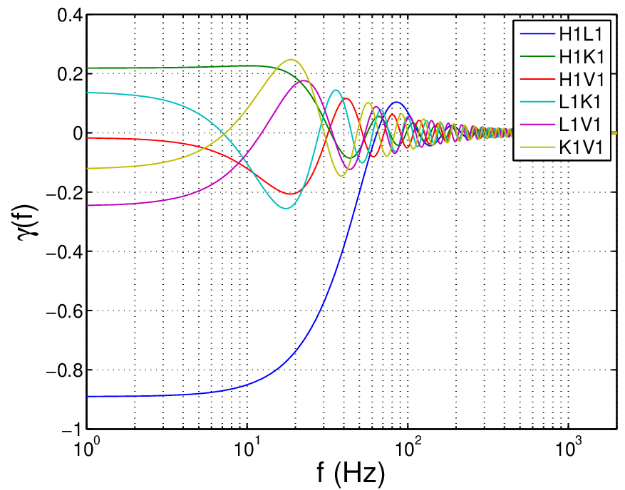
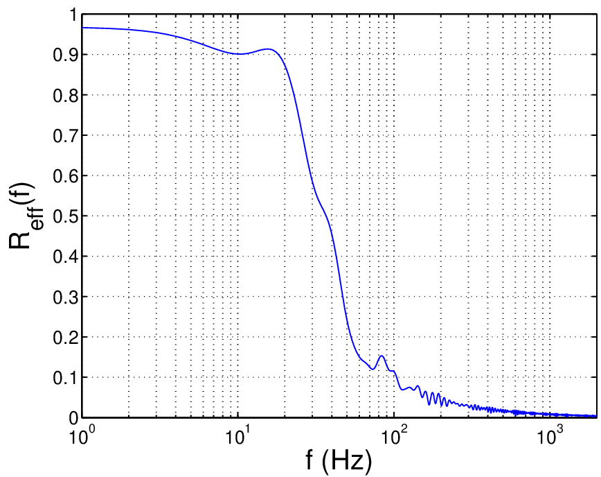
For the Advanced LIGO networks, we use the design detector noise power spectral density taken from [14] assumed to be the same for every detector in the network. We consider three networks: H1L1 (just the US aLIGO detectors), H1H2 (a hypothetical co-located pair of aLIGO detectors), and H1L1V1K1 (the US aLIGO detectors plus detector pairs created with Virgo V1 and KAGRA K1).55 5 We have taken the location and orientation of the KAGRA detector to be that of the TAMA 300-m interferometer in Tokyo, Japan. We have not included the planned LIGO India detector [16] in this network, as the precise LIGO-India site has not yet been decided upon. In reality, Virgo and KAGRA are expected to have different noise curves than aLIGO, but we assume the same aLIGO noise for each detector in order to show how the sensitivity curve changes by adding additional identical detectors to the network. Given this assumption, the effective strain power spectral density can be written as
| (31) |
where
| (32) |
is the sky- and polarization-averaged response of the network to a gravitational-wave background. A plot of the various overlap reduction functions and for the H1L1V1K1 network are given in Fig. 8.
 |
 |
The resulting power-law integrated sensitivity curves are shown in Fig. 9.

III.2.2 Big Bang Observer (BBO)
For the BBO sensitivity curve, the noise power spectral density for the two Michelson interferometers is taken to be
| (33) |
where
| (34) | ||||
| (35) |
are the position and acceleration noise (see Table II from [11]) and is the arm length. Following [12], we have included an extra factor of 4 multiplying the first term in Eq. 33, which corresponds to high-frequency noise 4 times larger than shot noise alone. The overlap reduction function for the Michelson interferometers located at opposite vertices of the BBO hexagram is shown in the right panel of Fig. 5. The power-law integrated curve for BBO is given in Fig. 10, top panel.
III.2.3 LISA
For LISA, the analysis is necessarily different since the standard cross-correlation technique used for multiple detectors such as an Advanced LIGO network, BBO, or a pulsar timing array is not possible for a single LISA constellation. This is because the two independent Michelson interferometers that one can synthesize from the six links of the standard equilateral LISA configuration are rotated at with respect one another, leading to zero cross-correlation for an isotropic gravitational-wave background for frequencies below about [17]. It is possible, however, to construct a combination of the LISA data whose response to gravitational waves is highly suppressed at these frequencies, and hence can be used as a real-time noise monitor for LISA [18, 19]. It is also possible to exploit the differences between the transfer function and spectral shape of a gravitational-wave background and that due to instrumental noise and/or an astrophysical foreground (e.g., from galactic white-dwarf binaries) to discriminate a gravitational-wave background from these other noise contributions [20, 21].
For the ideal case of an autocorrelation measurement in a single detector assuming perfect subtraction of instrumental noise and/or any unwanted astrophysical foreground, Eq. 21 for the expected signal-to-noise ratio is replaced by
| (36) |
where is the transfer function of the detector and is its noise power spectral density. (The reduction in compared to a cross-correlation analysis is due to the use of data from only one detector instead of two.) For standard LISA,
| (37) |
where
| (38) | ||||
| (39) |
are the position and acceleration noise [6, 11] and is the arm length. The transfer function is taken from Fig. 4 restricted to the LISA band, . Using the above expression for and following the same steps from the previous subsection for the construction of a power-law integrated curve, we obtain the sensitivity curve for LISA given in Fig. 10, middle panel.
Note that the minimum value of shown in this plot is about a factor of 10 times smaller than the value of reported in [20, 21]. Part of this difference is due to our use of for the sensitivity curve, while their value of corresponds to a strong (several ) detection having a Bayes factor . The remaining factor can probably be attributed to the marginalization over the instrumental noise and galactic foreground parameters in [20, 21], while Eq. 36 assumes that we know these parameters perfectly.
III.2.4 Pulsar timing array
For the pulsar timing array sensitivity curve, we consider a network of 20 pulsars taken from the International Pulsar Timing Network (IPTA) [22], which we assume have identical white timing noise power spectral densities,
| (40) |
where is the cadence of the measurements, taken to be , and is the root-mean-square timing noise, taken to be . We note that the pulsar timing network we envision may be somewhat optimistic as root-mean-square timing noise is ambitious. Also, we do not include the effects of fitting each pulsar’s period and spin-down rate to a timing model, which introduces both non-stationarity in the timing residuals and loss of sensitivity [23]. Nevertheless, one can still write down an analogous expression to Eq. 22 including these effects [24].
Since the timing noise power spectral densities are identical, it follows that
| (41) |
where
| (42) |
and are the Hellings and Downs factors for each pair of pulsars in the array. For our choice of 20 pulsars,
| (43) |
which can thought of as the effective number of pulsar pairs for the network. Finally, we assume a total observation time , which sets the lower frequency limit of . Given these parameters, we expect the pulsar timing array to be operating in the “intermediate signal limit” [24]. We therefore utilize the scaling laws from Fig. 2 in Ref. [24] to adjust the power-law integrated curves, since Eqs. 21, 22 for are valid in the weak-signal limit and overestimate the expected signal-to-noise ratio by a factor of for an observation of . The power-law integrated curve for IPTA is given in Fig. 10, bottom panel.
 |
 |
 |
It is interesting to note that the power-law integrated curves for Advanced LIGO and BBO are relatively round in shape, whereas the pulsar timing curve is pointy. (The steep spectrum can be understood as follows: the transfer function contributes a factor of while the conversion from power to energy density contributes an additional factor of .) This reflects the fact that the sensitivity of pulsar timing measurements is mostly determined by a small band of the lowest frequencies in the observing band regardless of the spectral shape of the signal. However, the timing-model fit mentioned above may round out the pointy shape of the PTA sensitivity curve. We also note that the stochastic background in the PTA band may exhibit variability. The power-law integrated curves represent the sensitivity to energy density observed at Earth over the course of the measurement.
Figure 11 is a summary the results of this section, showing the power-law integrated sensitivity curves for the different detectors on a single plot spanning a wide range of frequencies.

IV Discussion
We have presented a graphical representation of detector sensitivity curves for power-law gravitational-wave backgrounds that takes into account the enhancement in sensitivity that comes from integrating over frequency in addition to integrating over time. We applied this method to construct new power-law integrated sensitivity curves for cross-correlation searches involving advanced ground-based detectors, BBO, and a network of pulsars from a pulsar timing array. We also constructed a power-law integrated sensitivity curve for an autocorrelation measurement using LISA. The new curves paint a more accurate picture of the expected sensitivity of upcoming observations. The code that we used to produce the new curves is available at https://dcc.ligo.org/LIGO-P1300115/public for public download. Hopefully, this will allow other researchers to easily construct similar sensitivity curves. Required inputs are the noise power spectral density for each detector in the network and the overlap reduction function for each detector pair. Common default files are available for download with the plotting code.
Although the above discussion has focused on comparing predicted strengths of gravitational-wave backgrounds to sensitivity curves for current or planned detectors, one can also present measured upper limits for power-law backgrounds in a similar way. That is, instead of plotting the upper limits for (for fixed ) as a function of the spectral index as in [2, 25, 26], one can plot the envelope of upper-limit power-law curves as a function of frequency. This would better illustrate the frequency dependence of the upper limits in the observing band of the detectors.
Acknowledgements.
We thank Vuk Mandic and Nelson Christensen for helpful comments regarding an earlier draft of the paper. JDR would also like to thank Paul Demorest, Justin Ellis, Shane Larson, Alberto Sesana, and Alberto Vecchio for discussions related to PTA sensitivity curves. ET is a member of the LIGO Laboratory, supported by funding from United States National Science Foundation. LIGO was constructed by the California Institute of Technology and Massachusetts Institute of Technology with funding from the National Science Foundation and operates under cooperative agreement PHY-0757058. JDR acknowledges support from NSF Awards PHY-1205585, PHY-0855371, and CREST HRD-1242090.References
- [1] G. Hobbs, in High-Energy Emission from Pulsars and their Systems, edited by D. F. Torres and N. Rea (Springer Berlin Heidelberg, 2011), Astrophysics and Space Science Proceedings, p. 229.
- [2] B. Abbott et al., Nature 460, 990 (2009).
- [3] B. Allen and J. D. Romano, Phys. Rev. D 59, 102001 (1999).
- [4] N. Christensen, Physical Review D 46, 5250 (1992).
- [5] É. É. Flanagan, Physical Review D 48, 2389 (1993).
- [6] N. J. Cornish and S. L. Larson, Class. Quantum Grav. 18, 3473 (2001).
- [7] L. S. Finn, S. L. Larson, and J. D. Romano, Phys. Rev. D 79, 062003 (2009).
- [8] R. W. Hellings and G. S. Downs, Astrophys. J. Lett. 265, L39 (1983).
- [9] M. Anholm, S. Ballmer, J. D. E. Creighton, L. R. Price, and X. Siemens, Phys. Rev. D 79, 084030 (2009).
- [10] S. Phinney et al., NASA Mission Concept Study (2004).
- [11] J. Crowder and N. J. Cornish, Phys. Rev. D 72, 083005 (2005).
- [12] C. Cutler and J. Harms, Phys. Rev. D 73, 042001 (2006).
- [13] C. Wu, V. Mandic, and T. Regimbau, Phys. Rev. D 85, 104024 (2012).
- [14] D. Shoemaker, Advanced ligo anticipated sensitivity curves (2010), URL https://dcc.ligo.org/LIGO-T0900288/public.
- [15] J. Abadie et al., Class. Quantum Grav. 27, 173001 (2010).
- [16] B. Iyer et al., LIGO-India Tech. Rep. (2011), URL https://dcc.ligo.org/cgi-bin/DocDB/ShowDocument?docid=75988.
- [17] C. Cutler, Phys. Rev. D 57, 7089 (1998).
- [18] M. Tinto, J. W. Armstrong, and F. B. Estabrook, Phys. Rev. D 63, 021101 (2000).
- [19] C. J. Hogan and P. L. Bender, Phys. Rev. D 64, 062002 (2001).
- [20] M. R. Adams and N. J. Cornish, Phys. Rev. D 82, 022002 (2010).
- [21] M. R. Adams and N. J. Cornish (2013), http://arxiv.org/abs/1307.4116v2.
- [22] G. Hobbs et al., Class. Quantum Grav. 27, 084013 (2010).
- [23] R. van Haasteren and Y. Levin, Mon. Not. R. Ast. Soc. 428, 1147 (2013).
- [24] X. Siemens, J. Ellis, F. Jenet, and J. D. Romano, Class. Quantum Grav. 30, 224015 (2013).
- [25] J. Abadie et al., Phys. Rev. D 85, 122001 (2012).
- [26] V. Mandic, E. Thrane, S. Giampanis, and T. Regimbau, Phys. Rev. Lett. 109, 171102 (2012).