Sparsity-Promoting Sensor Selection for
Non-linear Measurement Models
Abstract
Sensor selection is an important design problem in large-scale sensor networks. Sensor selection can be interpreted as the problem of selecting the best subset of sensors that guarantees a certain estimation performance. We focus on observations that are related to a general non-linear model. The proposed framework is valid as long as the observations are independent, and its likelihood satisfies the regularity conditions. We use several functions of the Cramér-Rao bound (CRB) as a performance measure. We formulate the sensor selection problem as the design of a selection vector, which in its original form is a nonconvex -(quasi) norm optimization problem. We present relaxed sensor selection solvers that can be efficiently solved in polynomial time. We also propose a projected subgradient algorithm that is attractive for large-scale problems and also show how the algorithm can be easily distributed. The proposed framework is illustrated with a number of examples related to sensor placement design for localization.
Index Terms:
Sensor selection, sensor placement, Cramér-Rao bound, selection vector, sparsity, non-linear models, statistical inference, projected subgradient algorithm, convex optimization, sensor networks.I Introduction
Advances in sensor technology have enabled a large spectrum of applications and services related to safety and security, surveillance, environmental and climate monitoring, to list a few. The sensor nodes are spatially deployed and operate as a network, with each sensor node capable of sensing, processing, and communicating to other nodes or a central processing unit. As a network, their fundamental task is distributed data sampling (i.e., to sense the environment) from which we seek to extract relevant information. The sensors provide a prohibitively large dataset which is usually gathered at a fusion center. This gathered data has to be optimally processed, rejecting the redundant, identical, or faulty measurements.
Sensor selection is a fundamental design task in sensor networks. The number of sensors are often limited either by economical constraints (hardware costs), or the availability of physical or storage space. In order to reduce the hardware costs, as well as the resulting communications and processing overhead, one would like to smartly deploy the sensors. Sensor selection also enables the design of spatio-temporal sensing patterns that guarantee a certain performance measure such as energy-efficiency, information measure, estimation accuracy, or detection probability. The sensor placement problem can also be interpreted as a sensor selection problem in which the best subset of the available sensor locations are selected subject to a specific performance constraint. Sensor selection is pertinent to various diverse fields, especially to applications dealing with large-scale networks like network monitoring [2, 3], location-aware services like target localization and tracking [4, 5, 6], field estimation [7, 8], and environment monitoring in general. The fundamental questions of interest are:
- q1.
Where to deploy the limited sensors available?
- q2.
Do we need to process all the acquired measurements?
To this end, we focus on processing only the most informative sensors for a general non-linear statistical inference problem.
I-A Related prior works
A large volume of literature exists on sensor selection [9, and references therein]. The sensor selection problem is often formulated as an optimization problem based on some well-known performance measures from experimental design [10, 9], [11, Pg. 384]. The sensor selection problem is expressed as the following optimization problem:
| (1) |
where is a selection vector of length , and is a scalar cost function related to the mean squared error (MSE) covariance matrix . The MSE covariance matrix is optimized to select the best subset of sensors out of available sensors such that . Different functions can be used, and the typical choices for are related to:
- 1.
-
A-optimality: minimizes the sum of eigenvalues of with
- 2.
-
E-optimality: minimizes the maximum eigenvalue of with
- 3.
-
D-optimality: minimizes the determinant of with
This is a combinatorial optimization problem involving searches, and it is clearly intractable even for small-scale problems with and . To simplify this problem, the nonconvex Boolean constraint is relaxed to a convex box constraint . The relaxed optimization problem has been studied in [9] for additive Gaussian linear models, where the matrix is available in closed form, and more importantly, where the above listed performance measures are independent of the unknown parameter. Moreover, in practice, the exact number of sensors to select might not be known. However, this number can always be tuned to achieve a desired performance.
The above selection problem is applied to sensor placement for power grid monitoring in [12]. Alternative approaches exploiting the submodularity of the objective function [13, 14, 15], heuristics based on genetic algorithms [16], and greedy algorithms [17] are also proposed to solve the sensor selection problem. Sensor selection for dynamical systems often referred to as sensor polling or scheduling, is studied in [18, 19, 20]. In [21], the sensor placement problem for linear models is addressed as the design of a sensing matrix that optimizes a measure related to the orthogonality of its rows. All the above literature (in general) deals with measurements that are related to additive Gaussian linear models. Experimental design for non-linear models within the Bayesian and sequential design frameworks is discussed in [22]. In [18], sensor selection for target tracking based on extended Kalman filtering (EKF) has been proposed, in which the selection is performed by designing an appropriate gain matrix. Although a non-linear measurement model in additive Gaussian noise is used in [18], the past state estimate (not the true state) is used to compute the error covariance matrix leading to a suboptimal solution. Sensor selection for detection problems is studied in [23]. In [24], reliable sensor selection based on the actual measurements to identify the outliers is presented. A different problem, yet related to sensor selection, is the problem of identifying source-informative sensors, which is studied in [25].
I-B Contributions
The sensor selection problem can be interpreted as the problem to select the best sensors out of available sensors. The selected sensors are deemed as the best subset of sensors if they guarantee a certain specified estimation accuracy. We consider general scenarios where the measurements of the unknown parameter follow a non-linear model (unlike [9] for instance). Non-linear measurement models are frequently encountered in applications like source localization, tracking, field estimation, or phase retrieval, to list a few. The error covariance matrix for non-linear models is not always available in closed form, and more importantly it depends on the unknown parameter. Our first contribution in the context of sensor selection is to use the Cramér-Rao bound (CRB) as a performance measure. The CRB is a rigorous performance measure for optimality, and it generalizes very well for non-linear measurement models (not necessarily in additive Gaussian noise). Moreover, we do not need the actual measurements, and hence, our framework is also well-suited for solving offline design problems. In addition to this, the number of sensors that have to be selected, i.e., , is generally not known in practice. Hence, instead of fixing as in (1), we pose sensor selection as a cardinality minimization problem that provides the number of selected sensors as a byproduct. In order to do this, we use different thresholds that specify the required accuracy.
The proposed sensor selection framework is very generic and can be applied to any non-linear statistical inference problem (linear being a special case). The selection problem is formulated as the design of a selection vector which is an -(quasi) norm nonconvex Boolean optimization problem. It requires a brute-force evaluation over all the choices. For example, with available potential sensors, there are in the order of possible choices whose direct enumeration is clearly impossible. The nonconvex sensor selection problem is relaxed using standard convex relaxation techniques which can then be efficiently solved in polynomial time.
To cope with large-scale problems, we further present a projected subgradient algorithm. It is worth mentioning that the projected subgradient algorithm allows a very easy distributed implementation.
A sparsity-enhancing concave surrogate for the -(quasi) norm is also proposed for sensor selection as an alternative to the traditional best convex relaxation. This is particularly advantageous when there are multiple (nearly) identical sensor measurements. We illustrate the sensor selection problem using examples of sensor placement for source localization.
I-C Outline and notations
The remainder of the paper is organized as follows. In Section II, we present the non-linear measurement model. In Section III, we show the problem formulation, and we present the algorithms that solve the relaxed optimization problem in Section IV. In Section V, we derive the dual problem, and provide some extensions. In Section VI, the proposed framework is applied to a number of different models related to sensor selection for localization. The paper finally concludes with Section VII.
The notations used in this paper can be described as follows. Upper (lower) bold face letters are used for matrices (column vectors). denotes transposition. refers to a block diagonal matrix with the elements in its argument on the main diagonal. () denotes the vector of ones (zeros). is an identity matrix of size . denotes the expectation operation. is the matrix trace operator. is the matrix determinant. () denotes the minimum (maximum) eigenvalue of a symmetric matrix . means that is a positive semidefinite matrix. () denotes the set of symmetric (symmetric positive semi-definite) matrices of size . denotes the cardinality of the set .
II Non-linear measurement model
In this paper, we consider a generic non-linear measurement model
| (2) |
where is the th spatial or temporal sensor measurement, is the unknown parameter, for is the noise process, and the regressors for are (in general) non-linear functionals. Let the vector collect the measurements. The likelihood of the measurements is the probability density function (pdf) of parameterized by the unknown vector .
We make the following assumptions:
- a1.
-
Regularity conditions: The log-likelihood of the measurements satisfies the regularity condition . This is a well-known condition for the CRB to exist [26].
- a2.
-
Independent observations: The measurements for are a sequence of independent random variables.
The proposed framework for sensor selection is valid as long as the above two assumptions hold.
Assuming (a1) holds, the covariance of any unbiased estimate of the unknown parameter satisfies the well-known inequality [26]
where the Fisher information matrix (FIM) is given by
and is the CRB matrix. An important property of the Fisher information is that it is additive for independent observations, which follows from the fact that
| (3) |
where we assume that condition (a2) holds. Using (3), the FIM can be alternatively expressed as
which can be further simplified to
| (4) |
where
| (5) |
is the FIM of the th measurement. In other words, (4) means that every independent measurement contributes to the information measure. Note that the FIM for non-linear models depends on the unknown vector .
Assume for instance that the observations belong to the family of exponential distributions. The log-likelihood of the observations can then be expressed in the form
| (6) |
where and are known functions of the observations only, while and depend only on the unknown parameter. The regularity conditions in general hold for observations that belong to the family of exponential pdfs, and it already includes a large number of distributions.
One specific example that often occurs in practice is the case where the observations are related through the following additive Gaussian non-linear model
| (7) |
where is a non-linear function, and is a zero-mean Gaussian random variable with variance . The log-likelihood of is then given by (6) with
Assuming (a2) holds, it is then easy to verify that (5) simplifies to
Remark 1 (Additive Gaussian linear model).
As a special case, when the measurement process is linear, we have , i.e., with being the regressor. The computation of the FIM for a linear model is straightforward, and is given by
The CRB for linear models in additive Gaussian noise is also the MSE, and more importantly it is independent of the unknown vector.
III Problem formulation
Our goal is now to select the best subset () of the available sensor measurements such that a certain accuracy on the estimate is guaranteed. We next mathematically formulate this sensor selection problem.
III-A Sensor selection
In order to select the sensors, we introduce a selection vector
where indicates that the th sensor measurement is (not) selected. The measurement model including the virtual hard selection parameter can be visualized as
| (8) |
where the selection vector modifies the log-likelihood of the measurements as The corresponding FIM matrix in (4) can then be expressed as
| (9) |
III-B Performance measures
We do not restrict ourselves to any specific estimator, however, we use the CRB as a performance measure. The motivation behind using the CRB is as follows:
- 1.
The CRB is a measure for the (local) identifiability of the problem [27]. More specifically, a non-singular FIM implies (local) solvability and a unique estimate of , however, the converse is not necessarily true. The sensor selection problem presented in this paper seeks a subset of sensors for which the FIM has full rank in some domain such that the solvability of the problem in that domain is always ensured.
- 2.
Typically, the subset of selected sensors that yields a lower CRB also yields a lower MSE, and thus improves the performance of any practical system.
The CRB also has a very attractive mathematical structure resulting in a selection problem that can be efficiently solved using convex optimization techniques.
We next use the consistency assumption of the estimator to derive thresholds for the performance measures. We constrain the estimation error to be within an origin-centered circle of radius with a probability higher than , i.e.,
| (10) |
where denotes probability, and the values of and define the accuracy required and are assumed to be known. A higher accuracy level is obtained by reducing and/or increasing . This metric is used in several occasions as an accuracy measure (e.g., see [28, 4, 29]). We next discuss two popular performance measures that satisfy the above requirement.
III-B1 Trace constraint
III-B2 Minimum eigenvalue constraint
Another popular sufficient condition that also satisfies the accuracy requirement in (10) is
where is derived in [29] (see also Appendix A). This measure is related to the E-optimality. The inequality constraint can be equivalently expressed as the following linear matrix inequality (LMI):
| (11) |
In other words, we put a lower bound on each eigenvalue of the matrix . The solution set of satisfying this LMI is convex as and [11, Pg. 38].
The trace constraint has a larger feasible set as compared to the minimum eigenvalue constraint. However, although the trace constraint is a sufficient condition, the resulting sensor selection problem is computationally less attractive compared to the minimum eigenvalue constraint (as we show later). Moreover, LMIs can be used to also represent the trace constraint. For these reasons, we focus on the minimum eigenvalue (LMI) constraints from now on. However, without loss of generality (w.l.o.g.) either one of the two performance constraints can be used.
The above performance measures depend on the unknown parameter. In practice, the unknown parameter has a physical meaning and takes values within a certain domain denoted by . For example, in the case of direction-of-arrival estimation, is the sector where the source is expected or for target localization it is the surveillance area where the target resides. Since the FIM for non-linear models depends on the unknown , we propose to constrain every point within the domain .
Remark 2 (Bayesian CRB constraint).
In a Bayesian setting, when prior information of the unknown parameter is available, this additional knowledge typically yields a lower CRB, and the related information matrix is often called the Bayesian information matrix (BIM). The BIM is given by , where is some prior information matrix with the (log) prior . The LMI constraint in (11) for the Bayesian setting will then be
| (12) |
The prior information typically comes from the dynamics, previous measurements, or combining other available measurements.
III-C Problem statement
Having introduced the selection vector as well as the performance measure we can now formally state the problem.
Problem statement (Sensor selection).
Given the likelihoods of the measurements, and assuming (a1) and (a2) hold, find a vector that selects the minimum number of most informative sensors satisfying the performance measure .
In order to reduce the hardware costs, storage, processing, and communication overhead, we minimize the number of selected sensors. This can be achieved by minimizing the cardinality of the selection vector, i.e., by minimizing the number of non-zero entries of the selection vector. Mathematically, the sensor selection problem is formulated as the design of a selection vector which can be expressed as the following optimization problem
| (13a) | ||||
| (13b) | ||||
| (13c) | ||||
where the -(quasi) norm refers to the number of non-zero entries in , i.e., . The threshold imposes the accuracy requirement. The threshold is also the sparsity-inducing parameter, where implies a sparser solution.
Suppose the domain consists of points, obtained by gridding the entire domain at a certain resolution. The resulting multiple LMI constraints can be stacked together as a single LMI constraint. Let us consider the domain with . The constraints in (13b) can then be equivalently expressed as a single LMI constraint written as , where for . Note that the FIM after gridding is independent of , and we denote this simply by (not explicitly as a function of ).
Remark 3 (Worst-case constraints).
If there exists some such that and , then it is sufficient to constrain the performance for only the worst-case instead of . This property can be used a guideline for gridding.
IV Sensor selection solvers
It is well known that the -(quasi) norm optimization is NP-hard and nonconvex. More specifically, the original sensor selection problem in (13) is NP-hard. The Boolean constraint in (13c) is non-convex and incurs a combinatorial complexity. We next present a number of solvers with which the relaxed convex problem can be solved efficiently in polynomial time.
IV-A Convex approximation based on -norm
A computationally tractable (suboptimal) solution is to use the traditional best convex surrogate for the -(quasi) norm namely the -norm heuristic. The -norm is known to represent an efficient heuristic for the -(quasi) norm optimization with convex constraints especially when the solution is sparse [30]. Such relaxations are well-studied for problems with linear constraints in the context of compressed sensing (CS) and sparse signal recovery [31]. The non-convex Boolean constraint in (13c) is further relaxed to the convex box constraint .
The relaxed optimization problem is given as the following SDP problem
| (14a) | ||||
| (14b) | ||||
| (14c) | ||||
where denotes the -norm. Due to the positivity constraint, the objective function will simply be an affine function . The optimization problem in (14) is a standard SDP problem in the inequality form, which can be efficiently solved in polynomial time using interior-point methods [11]. An implementation of the interior-point method for solving SDP problems in the inequality form is typically based on Newton’s method using an approximating barrier function. A brief description of the projected Newton’s method is provided in Appendix C which is used to analyze the computational complexity of the relaxed sensor selection problem.
Remark 4 (Complexity per iteration).
The computational cost involved during each iteration is as follows [11, Pg. 619]. The matrices have a block-diagonal structure with blocks. Forming the matrix costs flops; computing via Cholesky factorization costs flops; the Hessian matrix is computed via the inner product of the matrices and , which costs . Finally, the Newton step is computed via Cholesky factorization costing flops, and the projection costs flops. Assuming that , the overall computational complexity per iteration of the projected Newton’s algorithm is then .
IV-B Projected subgradient algorithm
The second-order Newton’s method (cf. Appendix C) is typically intractable when the number of sensors is very large ( for example). To circumvent this problem, we propose a subgradient based algorithm. The projected subgradient algorithm is a first-order method which is attractive for large-scale problems as each iteration is much cheaper to process.
The subgradient method is typically used for optimizations involving non-differentiable functions [35, 36]. The subgradient method is a generalization of the gradient method for non-smooth and non-differentiable functions, such as, the -norm and the minimum eigenvalue constraint functions. We next derive the projected subgradient algorithm.
The relaxed sensor selection problem in (14) can be equivalently expressed as
| (15a) | ||||
| (15b) | ||||
| (15c) | ||||
where is the constraint function in (14b), and the set denotes the box constraints in (14c).
The objective is affine, so a subgradient of the objective is the all-one vector . Let denote a subgradient of the constraint function at . Here, the set denotes the subdifferential of evaluated at . To compute , we express the constraint function as
The computation of a subgradient is straightforward, and is given by
where is the eigenvector corresponding to the minimum eigenvalue . The minimum eigenvalue and the corresponding eigenvector can be computed using a low-complexity iterative algorithm called the power method (see Appendix D) or using the standard eigenvalue decomposition [37]. Let the projection of a point onto the set be denoted by , which can be expressed elementwise as
| (16) |
The projected subgradient algorithm then proceeds as follows:
| (17) |
In other words, if the current iterate is feasible (i.e., ), we update in the direction of a negative objective subgradient, as if the LMI constraints were absent; If the current iterate is infeasible (i.e., ), we update in the direction of a subgradient associated with the LMI constraints. After the update is computed, the iterate is projected onto the constraint set using .
When the th iterate is feasible, a diminishing non-summable step size is used. When the iterate is not feasible Polyak’s step size is used, where we adopt the optimal value for when known (i.e., the number of sensors to be selected is known). If this is not known, then we approximate it with , where , and [35]. The algorithm is terminated after a specified maximum number of iterations . Finally, the estimate is denoted by .
The convergence results of the subgradient method for the constrained optimization (i.e., without the projection step) are derived in [35]. Since the projection onto a convex set is non-expansive [36], it does not affect the convergence. The projected subgradient algorithm is summarized as Algorithm 1.
Remark 5 (Complexity per iteration).
We first form the matrix , which costs flops. The minimum eigenvalue and the corresponding eigenvector can be computed using the power method at a cost of flops [37]. Forming the vector costs flops, computing its norm costs flops, and the update and projection together cost flops. Assuming that as earlier, the computational cost of the projected subgradient algorithm is which is much lower than the complexity of the projected Newton’s method.
A distributed implementation of the projected subgradient algorithm is very easy. A simple distributed averaging algorithm (e.g., [38]) can be used to compute the sum of matrices . The minimum eigenvalue and the corresponding eigenvector can then be computed using power iterations at each node independently. The update equation (17), the subgradient vector , and the projection are computed coordinatewise and are already distributed.
Subgradient methods are typically very slow compared to the interior-point method involving Newton iterations, and subgradient methods typically require a few hundred iterations. Newton’s method typically requires in the order of ten steps. On the other hand, unlike the projected subgradient method, Newton’s method cannot be easily distributed, and requires a relatively high complexity per iteration due to the computation and storage of up to second-order derivatives. Depending on the scale of the problem and the resources available for processing one could choose between the subgradient or Newton’s algorithm.
IV-C Concave surrogate: sparsity-enhancing iterative algorithm
The -norm is customarily used as the best convex relaxation for the -norm. However, the intersection of the -norm ball (or an affine subspace) with the positive semi-definite cone (i.e., the LMI constraint) is not always a unique point as shown in the following Theorem.
Theorem 1 (Uniqueness).
The projection of a point onto a convex LMI constraint set under the -norm is not always unique.
Proof:
The proof follows from the fact that the -norm is not strictly convex, and from the linearity of the constraint set. Let us consider an example with (w.l.o.g.), and . In other words, the observations are identical. In this case, the extreme points of the -norm ball, i.e., and are two example solutions. Moreover, since the solution set of a convex minimization problem is convex, is also a solution for any , which gives an infinite number of solutions to the relaxed optimization problem (14). For such cases, the -norm relaxation will typically not result in a sparse solution. ∎To improve upon the -norm solution due to its non-uniqueness following from Theorem 1, we propose an alternative relaxation for the original sensor selection problem which also results in fewer selected sensors. Instead of relaxing the -(quasi) norm with the -norm, using a nonconvex surrogate function can yield a better approximation. It is motivated in [39] that the logarithm of the geometric mean of its elements can be used as an alternative surrogate function for linear inverse problems in CS. Adapting this to our sensor selection problem, we arrive at the optimization problem
| (18a) | ||||
| (18b) | ||||
| (18c) | ||||
where is a small constant that prevents the cost from tending to . The cost (18a) is concave, but since it is smooth w.r.t. , iterative linearization can be performed to obtain a local minimum [39]. The first-order approximation of around results in
Instead of minimizing the original cost, the majorizing cost (second term on the right-hand side of the above inequality) can be optimized to attain a local minima. More specifically, the optimization problem (18) can be iteratively driven to a local minimum using the iterations
| (19a) | ||||
| (19b) | ||||
| (19c) | ||||
The iterative algorithm is summarized as Algorithm 2. Each iteration in (19) solves a weighted -norm optimization problem. The weight updates force the small entries of the vector to zero and avoid inappropriate suppression of larger entries. The parameter provides stability, and guarantees that the zero-valued entries of do not strictly prohibit a nonzero estimate at the next step. Finally, the estimate is given by , where is the specified maximum number of iterations.
Remark 6 (Sparsity-enhancing projected subgradient algorithm).
The projected subgradient algorithm can be adapted to fit into the sparsity-enhancing iterative algorithm as well. The optimization problem (20) is then replaced with the following update equations:
where we solve a number of iterations (inner loop) of the projected subgradient algorithm within the th iteration (outer loop) of Algorithm 2. Here, the th iterate of the inner loop in the th outer loop is denoted as .
From the solution of the relaxed optimization problem, the approximate Boolean solution to can be obtained using randomization techniques, as described next.
| (20a) | ||||
| (20b) | ||||
| (20c) | ||||
IV-D Randomized rounding
The solution of the relaxed optimization problem is used to compute the suboptimal Boolean solution for the selection problem. A straightforward technique that is often used is the simple rounding technique, in which the Boolean estimate is given by where we define , and the operator rounds its arguments towards the nearest integer. However, there is no guarantee that the Boolean estimates obtained from the rounding technique always satisfy the LMI constraint. Hence, we propose a randomized rounding technique, where the suboptimal Boolean estimates are computed based on random experiments guided by the solution from the SDP problem in (14) or the iterative version in (19). The randomized rounding technique is summarized as Algorithm 3.
V Extensions
V-A The dual problem
The dual of the relaxed primal optimization problem has an interesting relation to the diameter of the confidence ellipsoids, and is closely related to the dual of the E-optimal design [11, Pg. 388]. The dual problem of (14) is given as follows
| (21) | ||||
where and are the dual variables, and we use with . For a detailed derivation of the dual problem, see Appendix B. The dual problem can be interpreted as the problem of maximizing the (average) diameter of the confidence ellipsoid. If we set , the optimal solution to the problem (21) is also the solution to the dual of the E-optimal design problem [11, Pg. 388], which maximizes the diameter of the confidence ellipsoid centered around the origin.
The dual formulation is often easier to solve and has only inequality constraints. The dual problem can be solved using Yalmip, SeDuMi, or CVX as earlier. Suppose and are dual feasible, and is primal feasible, then the dual problem yields the following bound on the primal SDP problem:
V-B Scalar constraints
Trace constraint
The relaxed sensor selection problem with the scalar trace constraint is given as follows
| (22) | ||||
The trace constraint in (22) is convex in ; this is easier to verify when the above trace constraint is expressed as an LMI [11, Pg. 387]. The optimization problem in (22) is a convex problem, and can be cast as an SDP:
| (23) | ||||
where is a variable, and is the th unit vector in . The optimization problem in (23) has LMI constraints for every point in and inequality constraints (in addition to the box constraint), while the optimization problem in (14) has only one LMI constraint for every point in (in addition to the box constraint). Hence, solving (23) is computationally more intense than solving (14).
Determinant constraint
Another popular scalar performance measure for the quality of the estimate is the determinant (product of eigenvalues) constraint. This measure is related to the D-optimality. The relaxed sensor selection problem with the determinant constraint is given as follows
| (24) | ||||
where the threshold specifies the mean radius a confidence ellipsoid (see Appendix A). In other words, although it is an indication of the performance of the estimator, it is not a sufficient condition for (10). The log-determinant constraint is a concave function of for for .
The relaxed sensor selection problem with the scalar (trace or determinant) constraints can be solved with either one of the two proposed cost functions, i.e., the -norm or the log-based concave surrogate.
VI Examples: Sensor placement for localization
Localization is an important and extensively studied topic in wireless sensor networks (WSNs). Target localization can be performed using a plethora of algorithms [4, 5, 6] (and references therein), which exploit inter-sensor measurements like time-of-arrival (TOA), time-difference-of-arrival (TDOA), angle-of-arrival (AOA), or received signal strength (RSS). The performance of any location estimator depends not only on the algorithm but also on the placement of the anchors (sensors with known locations). Sensor placement is a key challenge in localization system design, as certain sensor constellations not only deteriorate the performance but also result in ambiguity or identifiability issues [1].
The sensor placement problem can be interpreted as the problem where we divide a specific sensor area into grid points and select the best subset from these grid points. Here, the selected sensors are deemed the best, if they guarantee a certain minimal accuracy on the location estimates within a specific target area . We consider a two-dimensional network with one target located in the target area and possible sensors located at the grid points.
The absolute positions of the sensor grid points are known, hence, the considered sensors are commonly referred to as anchor nodes. Let the coordinates of the target and the th anchor be denoted by the vectors and , respectively, where is assumed to be unknown but known to be within . We next illustrate the proposed framework with a number of examples all related to localization.
VI-A Distance measurements
Let the pairwise distance between the target and the th anchor be denoted by . In practice, the pairwise distances are obtained by ranging and they are generally noisy. The range measurements generally follow an additive Gaussian non-linear model, as given by
| (25) |
where is the noise with . Here, is the nominal noise variance, and is the path-loss exponent. Using (9), we can now write the FIM for the localization problem as where using (5) we can compute
VI-B Received signal strength (RSS)
RSS is the voltage measured by a sensor’s received signal strength indicator (RSSI) circuit. RSS is often reported as the measured power. The ensemble mean received power at the th sensor can be expressed as
where is the received power (dBm) at a reference distance . However, due to shadowing, the difference between a measured received power and its ensemble average is random. The randomness due to shadowing is typically modeled as a log-normal process, which is Gaussian if expressed in decibels [6]. More specifically, the received power (dBm) at the th sensor follows a Gaussian distribution, i.e., . The FIM related to the th measurement is then given by
VI-C Bearing measurements
Another popular target localization technique is based on bearing measurements from a set of direction finding (DF) sensors [40]. The bearing measurement of the th DF sensor is given by
where , , and is the noise. Defining a permutation matrix , we can then compute the FIM contribution from the th DF sensor as
VI-D Energy measurements
Another popular localization scheme relevant to field estimation, (active/passive) radar, and sonar is to estimate the location of a point source that emits or reflects energy. Suppose the sensors measure the energy generated by a point source. The measurements are given as
| (26) |
where is the known energy emitted or reflected by the source, the known propagation function for some gain is modeled as an isotropic exponential attenuation , and is the noise. The FIM related to the th measurement is then given by
Remark 7 (Active sensor selection).
The sensor selection problem can also be formulated for active sensing. In active sensing, the sensors transmit probing signals (e.g., radar, sonar). The selection parameter for active sensing is a soft parameter used for joint selection and resource allocation [1], i.e., is a resource (e.g., transmit energy) normalized to the maximum prescribed value, and hence, it is dimensionless. The relaxed active sensor selection problem takes the same form as in (14). In fact, minimizing the -norm in active sensor selection minimizes the overall network resources (e.g., overall transmit energy).



VI-E Simulations
We apply the proposed sensor selection problem to sensor placement design for target localization. To test the proposed algorithms, we use CVX [34]. CVX internally calls SeDuMi [33], a MATLAB implementation of the second-order interior-point methods.
We consider the scenario shown in Fig. 1a with sensors to illustrate the sensor selection problem. Recall that the problem here is to choose the best sensor positions out of available ones, such that a certain specified localization accuracy is achieved. The domain for this example will be the target (or surveillance) area where the target resides, and to avoid having infinitely many constraints the area consists of grid points at a certain resolution. We grid the target area of uniformly with a resolution of m along both horizontal and vertical directions as shown in Fig. 1a.
The original non-convex sensor selection problem is relaxed to an -norm optimization problem. Alternatively, a concave surrogate function can be used to enhance the sparsity. The optimization problem with the concave surrogate cost function is iteratively solved by affinely scaling the objective based on the solution from the previous iteration. For the sparsity-enhancing iterative Algorithm 2, we use and . The number of candidates used in the randomized rounding Algorithm 3 is . As observed in the simulations, a solution is typically found in the first batch itself, and a few tens of candidate entries are sufficient. We use the following parameters for the simulations: , , square-degrees, dB, dBm, , , and (except in Fig. 1d).
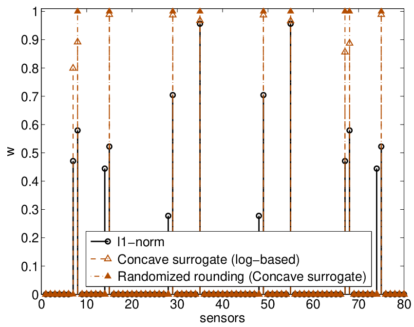
Fig. 1 shows the sensor selection for the distance (range) measurement model. The thresholds are computed with cm and . The selection shown in Fig. 1a is based on Algorithm 2 with randomized rounding to recover the approximate Boolean solution. The selection results based on the -norm cost with the minimum eigenvalue constraint is shown in Fig. 1b. Fig. 1b also shows that the solution based on the concave surrogate cost function with the minimum eigenvalue constraint leads to a sparser solution. The selection results based on the trace constraint obtained by solving (22) are illustrated in Fig. 1c. The sensors from the same region (close to the red filled boxes in Fig. 1a) are selected with both constraints. Fig. 1d shows a zero-duality gap (gap between the cost of the primal problem in (14) and the dual problem in (21)) for different values of . Larger values of result in a larger , and subsequently more sensors are selected. The sufficient trace constraint has a larger feasible set compared to the stronger sufficient minimum eigenvalue constraint. As a result, for the considered scenario, the minimum eigenvalue constraint leads to a slightly larger -norm compared to the trace constraint.
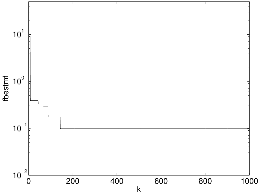
The optimization problem (14) is also solved using the projected subgradient method summarized in Algorithm 1 with iterations. The solution of the projected subgradient is shown in Fig. 2a. The performance of the projected subgradient algorithm is compared to the solution of the interior-point methods (implemented using SeDuMi) denoted by (obtained via SeDuMi), i.e., is shown in Fig. 2b. Even though the convergence of the projected subgradient algorithm is very slow, the estimated support after a few hundred iterations can be used along with randomized rounding to further refine the solution. The computation time on the same computer for the projected subgradient algorithm that solves (14) is around seconds for iterations while SeDuMi takes around seconds to solve the SDP problem in (14).

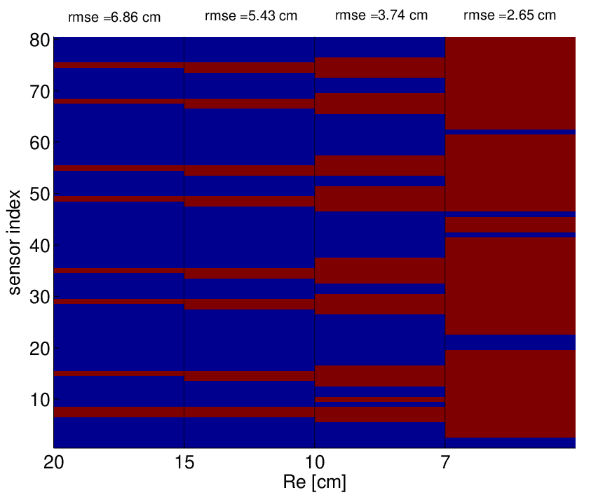

A practical estimator does not meet the CRB in some cases (for instance at low SNRs or finite data records). Therefore, the sensors obtained with a specific would lead to an underestimate of the desired MSE. We can account for this gap by choosing appropriately. To this end, we give the entire solution path of the selected sensors for different values of in Fig. 3a. The solution path can be efficiently computed by increasing . The sensors corresponding to some can then be used to meet the desired MSE requirement. The non-linear model in (25) is solved in the least-squares sense iteratively using Gauss-Newton’s method with iterations [26]. The maximum root-MSE (RMSE), maximum root-CRB, average RMSE, and average CRB of the location estimates of a target within the target area using the selected sensors (as shown in the solution path) for different values of are shown in Fig. 3b. For the considered scenario, both the maximum and average root-CRB satisfy the performance constraint which is given by the inequality in (27). The performance constraint is shown as a red solid line in Fig. 3b. The maximum RMSE does not satisfy the accuracy requirement specified by a certain , and this can be corrected by using an appropriate (lower) . Moreover, for the considered scenario, the gap between the average RMSE and the performance constraint is still reasonable. We also show the maximum RMSE on top of Fig. 3a.
The proposed framework is very general, and can be applied to a variety of data models as long as (a1) and (a2) are valid. To illustrate this we next consider a few more measurement models. The sensor selection based on bearing measurements is illustrated in Fig. 4. Here, we use cm, and . The selection results for the RSS based measurement model is shown in Fig. 5. We use dB, , and m. Sensor selection results based on energy measurements are shown in Fig. 6, where we use cm, and . An illustration of the field generated by a point source at location m with unit amplitude is also shown here.
The FIM for all the considered measurement models has a common structure, and it decreases as the distance increases. However, the rate at which it decreases is different for different models. Anyway, as a result of this decrease, the optimization problem leads to a sensor selection that is close to the target area (in the Euclidean distance sense) for all the considered models.


VII Conclusions
Sensor selection is an important design problem in sensor networks. The sensor selection problem can be described as the problem of selecting the best subset of sensors that guarantees a certain specified performance measure. The sensor selection enables deployment of the sensors with guarantees on the resulting estimation accuracy. This also minimizes the hardware, communications, and resulting processing costs in large-scale networks. We focus on observations that follow a non-linear model. The proposed framework is valid as long as the observations are independent, and their pdfs are regular. We use a number of functions related to the FIM as a performance measure. The original nonconvex optimization problem is relaxed using convex relaxation techniques which can then be efficiently solved in polynomial time. To handle large-scale problems, we have also presented a projected subgradient algorithm. This also enables easy distributed implementations. The proposed framework is applied to sensor placement design for a number of different models related to localization.
Appendix A Performance thresholds
Trace and minimum eigenvalue constraints
We can relate the accuracy requirement and the CRB using Chebyshev’s inequality [28]
which can be equivalently expressed as . Combining this inequality together with in (10) results in the following sufficient condition
| (27) |
Each eigenvalue of is greater than , and as a result, . Hence, a stronger sufficient condition (with a smaller feasible set) is , or equivalently [29]
Determinant constraint
The determinant constraint is related to the volume or the mean radius of the confidence ellipsoid that contains with probability . Such a confidence ellipsoid can be expressed as
where is a constant that depends on . Assuming has ordered eigenvalues , the length of the th semi-axis of the ellipsoid will be . The geometric mean radius of the confidence ellipsoid given by
gives a quantitative measure of how informative the observations are. For the estimates to be within the confidence ellipsoid , we use the constraint
where and specify the required accuracy, and are assumed to be known. A typical choice for is constant chi-squared values, i.e., . Here, is the cumulative distribution function of a chi-squared random variable with degrees of freedom. This performance measure is related to the D-optimality.
Appendix B Derivation of the dual problem
Consider the optimization problem (14) as the primal problem. To this problem, we then associate the following dual variables or Lagrangian multipliers: with the LMI constraint; and with the and constraints, respectively. The Lagrangian is
The Lagrange dual function
is given as (29). The dual problem which is also an SDP can therefore be expressed as
where (we use the fact that is self-dual), and are the dual variables. By eliminating , the dual problem is simplified to
| (28a) | ||||
| (28b) | ||||
| (28c) | ||||
| (29) |
Appendix C Projected Newton’s method
In order to analyze the complexity of the interior point methods, we briefly describe the projected Newton’s method. The Newton’s method for an SDP problem in the inequality form is adapted to suit our problem [11, Pg. 619].
The optimization problem in (14) can be approximated using the log-determinant barrier function which is given as
where is a parameter to tune the approximation. The projected Newton’s update equation is given by
| (30) |
where the entries of the Hessian matrix are given by
and the entries of the gradient vector are given by
Here, we have introduced the matrix , and recall the projector operator defined in (16). The step-length is chosen by line-search.
Appendix D Power iterations for computing the minimum eigenvalue
We briefly describe the power iterations [37] to compute the minimum eigenvalue of a matrix . Assuming has ordered eigenvalues , the power iterations
converge to the eigenvector corresponding to the maximum eigenvalue , and the maximum eigenvalue , respectively, as . Here, we use . By forming a matrix which has the dominant eigenvalue , we can apply the above power iterations on to compute and , and thus the minimum eigenvalue of F and it’s corresponding eigenvector.
References
- [1] S. P. Chepuri, G. Leus, and A.-J. van der Veen, “Sparsity-exploiting anchor placement for localization in sensor networks,” in Proc. of the 21st European Signal Processing Conference (EUSIPCO), Sept. 2013.
- [2] G. Mateos and K. Rajawat, “Dynamic network cartography: Advances in network health monitoring,” IEEE Signal Process. Mag., vol. 30, no. 3, pp. 129–143, 2013.
- [3] G. B. Giannakis, V. Kekatos, N. Gatsis, S.-J. Kim, H. Zhu, and B. F. Wollenberg, “Monitoring and optimization for power grids: A signal processing perspective,” IEEE Signal Process. Mag., 2013.
- [4] F. Gustafsson and F. Gunnarsson, “Mobile positioning using wireless networks: possibilities and fundamental limitations based on available wireless network measurements,” IEEE Signal Process. Mag., vol. 22, no. 4, pp. 41 – 53, July 2005.
- [5] S. Gezici, Z. Tian, G. B. Giannakis, H. Kobayashi, A. F. Molisch, H. V. Poor, and Z. Sahinoglu, “Localization via ultra-wideband radios: a look at positioning aspects for future sensor networks,” IEEE Signal Process. Mag., vol. 22, no. 4, pp. 70–84, July 2005.
- [6] N. Patwari, J. N. Ash, S. Kyperountas, A. O. Hero III, R.L. Moses, and N.S. Correal, “Locating the nodes: cooperative localization in wireless sensor networks,” IEEE Signal Process. Mag., vol. 22, no. 4, pp. 54 – 69, Jul. 2005.
- [7] T. van Waterschoot and G. Leus, “Static field estimation using a wireless sensor network based on the finite element method,” in Proc. of 4th IEEE International Workshop on Computational Advances in Multi-Sensor Adaptive Processing (CAMSAP), 2011, pp. 369–372.
- [8] Haotian Zhang, J.M.F. Moura, and B. Krogh, “Dynamic field estimation using wireless sensor networks: Tradeoffs between estimation error and communication cost,” IEEE Trans. Signal Process., vol. 57, no. 6, pp. 2383–2395, 2009.
- [9] S. Joshi and S. Boyd, “Sensor selection via convex optimization,” IEEE Trans. Signal Process., vol. 57, no. 2, pp. 451–462, Feb. 2009.
- [10] F. Pukelsheim, Optimal design of experiments, vol. 50, SIAM, 1993.
- [11] S. Boyd and L. Vandenberghe, Convex Optimization, Cambridge University Press, New York, NY, USA, 2004.
- [12] V. Kekatos, G.B. Giannakis, and B. Wollenberg, “Optimal placement of phasor measurement units via convex relaxation,” IEEE Trans. Power Syst., vol. 27, no. 3, pp. 1521–1530, 2012.
- [13] A. Krause, A. Singh, and C. Guestrin, “Near-optimal sensor placements in gaussian processes: Theory, efficient algorithms and empirical studies,” The Journal of Machine Learning Research, vol. 9, pp. 235–284, 2008.
- [14] A. Krause and C. Guestrin, “Near-optimal observation selection using submodular functions,” in AAAI, 2007, vol. 7, pp. 1650–1654.
- [15] A. Krause, H.B. McMahan, C. Guestrin, and A. Gupta, “Robust submodular observation selection.,” Journal of Machine Learning Research, 2008.
- [16] L. Yao, W.A. Sethares, and D.C. Kammer, “Sensor placement for on-orbit modal identification via a genetic algorithm,” AIAA journal, vol. 31, no. 10, pp. 1922–1928, 1993.
- [17] M. Shamaiah, S. Banerjee, and H. Vikalo, “Greedy sensor selection: Leveraging submodularity,” in Decision and Control (CDC), 2010 49th IEEE Conference on. IEEE, 2010, pp. 2572–2577.
- [18] E. Masazade, M. Fardad, and P.K. Varshney, “Sparsity-promoting extended kalman filtering for target tracking in wireless sensor networks,” IEEE Signal Process. Lett., vol. 19, no. 12, pp. 845–848, 2012.
- [19] A. Carmi, “Sensor scheduling via compressed sensing,” in Proc. of 13th Conference on Information Fusion (FUSION), 2010, pp. 1–8.
- [20] Yinfei Fu, Qing Ling, and Zhi Tian, “Distributed sensor allocation for multi-target tracking in wireless sensor networks,” IEEE Trans. Aerosp. Electron. Syst., vol. 48, no. 4, pp. 3538–3553, 2012.
- [21] J. Ranieri, A. Chebira, and M. Vetterli, “Near-optimal sensor placement for linear inverse problems,” IEEE Trans. Signal Process., vol. 62, no. 5, pp. 1135–1146, March 2014.
- [22] I. Ford, D. M. Titterington, and Christos P. Kitsos, “Recent advances in nonlinear experimental design,” Technometrics, vol. 31, no. 1, pp. 49–60x, 1989.
- [23] D. Bajovic, B. Sinopoli, and J. Xavier, “Sensor selection for event detection in wireless sensor networks,” IEEE Trans. Signal Process., vol. 59, no. 10, pp. 4938–4953, Oct 2011.
- [24] V. Kekatos and G.B. Giannakis, “From sparse signals to sparse residuals for robust sensing,” IEEE Trans. Signal Process., vol. 59, no. 7, pp. 3355–3368, 2011.
- [25] I.D. Schizas, “Distributed informative-sensor identification via sparsity-aware matrix decomposition,” IEEE Trans. Signal Process., vol. PP, no. 99, pp. 1–1, 2013.
- [26] S. M. Kay, Fundamentals of Statistical Signal Processing: Estimation Theory, Englewood Cliffs, NJ: Prentice-Hall, 1993.
- [27] T.J. Rothenberg, “Identification in parametric models,” Econometrica: Journal of the Econometric Society, pp. 577–591, 1971.
- [28] Thomas M Cover and Joy A Thomas, Elements of information theory, John Wiley & Sons, 2012.
- [29] T. Wang, G. Leus, and L. Huang, “Ranging energy optimization for robust sensor positioning based on semidefinite programming,” IEEE Trans. Signal Process., vol. 57, no. 12, pp. 4777 –4787, Dec. 2009.
- [30] B. Polyak, M. Khlebnikov, and P. Shcherbakov, “An lmi approach to structured sparse feedback design in linear control systems,” in The European Control Conference, 2013.
- [31] D.L. Donoho, “For most large underdetermined systems of linear equations the minimal -norm solution is also the sparsest solution,” Communications on pure and applied mathematics, vol. 59, no. 6, pp. 797–829, 2006.
- [32] J. Lfberg, “Yalmip : A toolbox for modeling and optimization in MATLAB,” in Proceedings of the CACSD Conference, Taipei, Taiwan, 2004.
- [33] Jos F. Sturm, “Using SeDuMi 1.02, a matlab toolbox for optimization over symmetric cones,” 1998.
- [34] M. Grant and S. Boyd, “CVX: Matlab software for disciplined convex programming, version 2.0 beta,” http://cvxr.com/cvx, Sept. 2012.
- [35] S. Boyd, L. Xiao, and A. Mutapcic, “Subgradient methods,” http://www.stanford.edu/class/ee364b/notes/subgrad_method_notes.pdf, 2003.
- [36] D. P. Bertsekas, Nonlinear programming, Athena Scientific optimization and computation series. Athena Scientific, 1999.
- [37] G. H. Golub and C. F. Van Loan, Matrix Computations, Johns Hopkins Studies in the Mathematical Sciences. Johns Hopkins University Press, 1996.
- [38] Lin Xiao and S. Boyd, “Fast linear iterations for distributed averaging,” Systems & Control Letters, vol. 53, no. 1, pp. 65–78, 2004.
- [39] E. Candés, M. Wakin, and S. Boyd, “Enhancing sparsity by reweighted minimization,” Journal of Fourier Analysis and Applications, vol. 14, pp. 877–905, 2008.
- [40] M. Gavish and A.J. Weiss, “Performance analysis of bearing-only target location algorithms,” IEEE Trans. Aerosp. Electron. Syst., vol. 28, no. 3, pp. 817–828, Jul 1992.