跳到论文正文
W Papers独立论文阅读器 arXiv:1310.5248 论文正文 计算阅读时间 · 0%
引用这篇论文根据当前论文元数据生成,正式投稿前建议核对。


License: arXiv.org perpetual non-exclusive license
arXiv:1310.5248v2 [cond-mat.quant-gas] 22 Oct 2013

Probing many-body interactions in an optical lattice clock

A. M. Rey1∗, A. V. Gorshkov2, C. V. Kraus3,4, M. J. Martin1,5, M. Bishof1, M. D. Swallows1, X. Zhang1, C. Benko1, J. Ye1, N. D. Lemke6 and A. D. Ludlow6 Affiliation: 1JILA, NIST and University of Colorado, Department of Physics, Boulder, CO 80309, USA Affiliation: ∗ E-mail: arey@jilau1.colorado.edu Affiliation: 2 Joint Quantum Institute, NIST and University of Maryland, Department of Physics, College Park, MD 20742, USA Affiliation: 3Institute for Quantum Optics and Quantum Information of the Austrian Academy of Sciences, A-6020 Innsbruck, Austria Affiliation: 4Institute for Theoretical Physics, University of Innsbruck, A-6020 Innsbruck, Austria Affiliation: 5Institute for Quantum Information and Matter, California Institute of Technology, Pasadena, CA 91125, USA Affiliation: 6National Institute of Standards and Technology, Boulder, CO 80305, USA
August 24, 2026
Abstract

We present a unifying theoretical framework that describes recently observed many-body effects during the interrogation of an optical lattice clock operated with thousands of fermionic alkaline earth atoms. The framework is based on a many-body master equation that accounts for the interplay between elastic and inelastic pp-wave and ss-wave interactions, finite temperature effects and excitation inhomogeneity during the quantum dynamics of the interrogated atoms. Solutions of the master equation in different parameter regimes are presented and compared. It is shown that a general solution can be obtained by using the so called Truncated Wigner Approximation which is applied in our case in the context of an open quantum system. We use the developed framework to model the density shift and decay of the fringes observed during Ramsey spectroscopy in the JILA 87Sr and NIST 171Yb optical lattice clocks. The developed framework opens a suitable path for dealing with a variety of strongly-correlated and driven open-quantum spin systems.

I Introduction

One of the ultimate goals of modern physics is to understand and fully control quantum mechanical systems and to exploit them both, at the level of basic research and for numerous technological applications including navigation, communications, network management, etc. To accomplish these objectives, we aim at developing the most advanced and novel measurement techniques capable of probing quantum matter at the fundamental level.

Some years ago, the second – the international unit of time – was defined by the Earth’s rotation. However, with the discovery of quantum mechanics and the quantized nature of the atomic energy levels, it became clear that atomic clocks could be more accurate and more precise than any mechanical or celestial reference previously known to man. Thus, in 1967 the second was redefined as the duration of 9,192,631,770 periods of the radiation corresponding to the transition between the two hyperfine energy levels of a caesium atom. Since then, the accuracy of atomic clocks has improved dramatically, by a factor of 10 or so every decade. The characterization of the unit of time plays a central role within the International System of Units (SI) because of its unprecedented high accuracy and because it is also used in the definitions of other units such as meter, volt and ampere.

Thanks to the development of laser trapping and cooling techniques [1, 2], the best caesium standards have reached an accuracy of one part in 101610^{16}. However, caesium clocks are limited by the fact that they are based on atomic transitions in the microwave domain. Because the quality factor of the clock is proportional to the frequency, optical clocks with frequencies that can be 10610^{6} times higher than microwaves, offer an impressive potential gain over their microwave counterparts. Optical frequencies on the other hand are very difficult to measure, as the oscillations are orders of magnitude faster than what electronics can measure. The implementation of frequency comb technology [3] has provided a coherent link between the optical and microwave regions of the electromagnetic spectrum, greatly simplifying optical frequency measurements of high accuracy. After the development of frequency combs, the interest in optical clocks has grown rapidly. Now, optical clocks based on single trapped ions and neutral atoms are the new generation of frequency standards with a sensitivity and accuracy as high as one part in 101810^{18} [4, 5, 6].

Optical clocks operated with fermionic neutral alkaline earth atoms (AEA), such as 87Sr or 171Yb, have matured considerably. Those employ an optical lattice to tightly confine the atoms so that Doppler and photon-recoil related effects on the transition frequency are eliminated. State-of-the-art neutral-atom-optical clocks have surpassed the accuracy of the Cs standard [7] and just recently, thanks to advances in modern precision laser spectroscopy, are reaching and even surpassing the accuracy of single ion standards [6]. The most stable of these clocks now operate near the quantum noise limit [8, 9]. The stability arises from the intrinsic atomic physics of two-valence-electron atoms that possess extremely long lived singlet and triplet states (clock states), with intercombination lines nine orders of magnitude narrower than a typical dipole-allowed electronic transition.

The potential advantage of neutral-atom clocks over single trapped ion clocks is that, in the former, a large number of atoms is simultaneously interrogated. This could lead to a large signal-to-noise improvement; however, high atom numbers combined with tight confinement also lead to high atomic densities and the potential for non-zero collisional frequency shifts via contact atom- atom interactions. With atom-light coherence times reaching several seconds, even very weak interactions (e.g., fractional energy level shifts of order ≥1×10⁻¹⁶\geq 1\times 10^{-16}) can dominate the dynamics of these systems.

To suppress these interactions, the use of ultracold, spin-polarized fermions was proposed. The idea was to exploit the Fermi suppression of ss-wave contact interactions while freezing out pp-wave and higher wave collisions at ultracold atomic temperatures. Indeed, at precision level of 10−1510^{-15}, the JILA Sr clock did not exhibit a density-dependent frequency shift [10], however as the measurement precision progressed, density-dependent frequency shifts were measured in spin polarized fermions, at the JILA Sr clock [11, 12, 13] and at the NIST Yb clock [14].

When those density-dependent frequency shifts were first observed, they were attributed to ss-wave collisions allowed by inhomogeneous excitation [15, 11, 16, 17, 18], under the assumption that pp-wave interactions were suppressed at the operating temperatures (T∼μT\sim\muK) [11]. The basic initial understanding, obtained from a mean-field treatment, was that excitation inhomogeneities induced by the optical probing laser made the initially indistinguishable fermionic atoms distinguishable, and thus allowed them to interact via ss-wave collisions.

However, studies of the cold collision shift in the NIST Yb optical lattice clock using Ramsey spectroscopy revealed that pp-wave interactions were the dominant elastic interactions in that system [19]. Furthermore, evidence of inelastic pp-wave interactions was reported in both Yb and Sr atomic clocks [20, 21]. Although the importance of many-body interactions in optical clocks has been recognized theoretically [16, 17, 18], only recent measurements have revealed their many-body nature [22, 23]. In those measurements, the role of ss-wave collisions was further suppressed by operating the Sr clock with highly homogeneous atom-laser coupling. This results in dominant pp-wave interactions with a collective character, as we will explain below.

At this point it is important to emphasize that recent advances in modern precision laser spectroscopy, with record levels of stability and residual laser drift less than mHz/s [8, 24, 23] are the crucial developments that are allowing us to deal with clocks operated at a very different conditions than those ones dealt with just few years ago. The level of precision spectroscopy achievable in current atomic clocks is now providing the required spectral resolution to systematically resolve and study the complex excitation spectrum of an interacting many-body system. This was certainly not the case in prior clock experiments where interaction effects were subdominant and where a mean-field treatment was more than enough to describe the clock behavior. For example in 2006, a 2 Hz spectral resolution has achieved for the Sr atomic transition and no interaction effects were observable at the time [25].

In this paper we present a unifying theoretical framework that goes beyond a simple mean-field treatment and that is capable of describing the full many-body dynamics of nuclear spin-polarized alkaline earth atoms during clock interrogation. The two clock states are treated as an effective spin degree of freedom. Both, elastic and inelastic two-body collisions and single-particle losses are present during the dynamics, and thus a pure Hamiltonian formulation is not sufficient. Instead, we develop a master equation formulation which is capable of treating the quantum evolution of an open spin system. We provide analytic/exact solutions of the master equation dynamics in parameter regimes where exact treatments are possible. For the more generic situations we solve the dynamics relying on the so called Truncated Wigner Approximation (TWA) [26, 27]. In contrast to previous theoretical treatments of the clock dynamics, which were limited to treating two-particles or many-particles but at the mean-field level or under the all-to-all approximation [16, 17, 16, 17, 18, 13], the TWA method allows us to include both elastic and inelastic collisions beyond the mean-field level, finite temperature effects and inhomogeneities generated by either the laser during the pulse interrogation or by many-body interactions. Those are shown to be crucial for properly modeling observed many-body dynamics, especially at T≳10​μT\gtrsim 10\muK, at which excitation inhomogeneities can not be neglected. To our knowledge this is the first time that the TWA is applied to describe an open quantum system in the presence of inelastic losses.

Although this paper focuses on optical lattice clocks, the developed theoretical framework is generic for driven open-quantum systems and should be a useful platform for dealing with a variety of current experimentally relevant systems including trapped ions [28, 29], polar molecules [30, 31, 32, 33, 34, 35], nitrogen vacancy centers [36], and atoms in optical cavities [37, 38] among others.

Refer to caption
Figure 1: (Color online) General design of an optical lattice clock

The remainder of the paper is organized as follows. In section II, we introduce the reader to the basic operation of an atomic clock and derive the many-body Hamiltonian that describes the dynamics of nuclear spin-polarized fermionic atoms during clock interrogation. We then proceed to derive a simplified effective spin model which assumes frozen motional-excitations during the dynamics. In section III, we solve for the dynamics under the assumption of collective spin interactions (all-to-all interactions) in a closed system. In Section IV, we show how to treat the observed two-body losses and introduce a master equation, which we solve under the collective-interactions approximation. We also show how to use the TWA to deal with the open quantum system dynamics. In section V, we relax the frozen-motional-degrees-of-freedom approximation and derive an improved spin Hamiltonian with cubic spin-spin interactions which account for the virtual occupation of excited motional modes. In section VI, we go beyond the all-to-all interactions approximation and present a more general prescription that can address both non-collective interactions and losses and single-particle inhomogeneities. In section VII, we apply the developed theoretical framework to model the dynamics during Ramsey spectroscopy observed in the JILA87Sr and the NIST 171Yb optical lattice clocks, and finally, in section VIII, we present the conclusions. In Appendixes 1-5, we present some details omitted in the main text.

II Many-body physics during clock operation

II.1 A simple overview of an optical lattice clock

The general design of an optical lattice clock is shown in Fig. 1. It consists of two components, a laboratory radiation source and an atomic system with a natural reference frequency determined by quantum mechanics to which the laboratory radiation source can be compared. Here, the laboratory radiation source is an ultra-stable continuous-wave laser. It acts as the local oscillator (or pendulum) for the clock and is used to probe an electromagnetic resonance in an atom. The atomic signal can then be used to determine the difference between the laser frequency and that of the reference atom, allowing laser frequency to be monitored and stabilized to the preferred value. A frequency comb [3] provides the gears of the clock, allowing measurements of the laser frequency relative to other high accuracy clocks in either the optical or microwave domains.

The two main quantities that characterize the performance of a clock are the accuracy and the precision. The accuracy is determined by how well the measured frequency matches that of the atom’s natural frequency. In general, the accuracy will depend on the atomic species used and how well it can be isolated from environmental effects during spectroscopy. The precision of the clock is more commonly referred to as the stability, which represents the repeatability of the measured clock frequency over a given averaging time τ\tau. For quantum projection noise limited measurements, it is typically expressed as [39]

σ⁡(τ)≈Δ​νν​tcτ​N.\sigma(\tau)\approx\frac{\Delta\nu}{\nu}\sqrt{\frac{t_{c}}{\tau N}}. (1)

Here, νΔ​ν=Q\frac{\nu}{\Delta\nu}=Q is the line quality factor of the clock transition for a linewidth Δ​ν\Delta\nu and N\sqrt{N} is associated with the signal-to noise-ratio achieved for interrogating NN atoms in the measurement cycle time tct_{c}.

Fermionic AEA such as 87Sr and 171Yb have unique properties that make them ideal candidates for the realization of atomic clocks [40]. The clock states are the ground singlet state, S01{}^{1}S_{0}, and a long lived triplet state P03{}^{3}P_{0}, with intercombination lines both electric and magnetic dipole forbidden and as narrow as a few mHz, see Fig. 2. In the ground state (S01{}^{1}S_{0}), and to leading order in the excited state (P03{}^{3}P_{0}), the electronic degrees of freedom have neither spin nor orbital angular momentum [25]. This means that the atoms in the clock states only interact with external magnetic fields through the nuclear spin degrees of freedom which have a gg-factor 1000 times smaller than the electronic orbital one. Therefore, AEA are much less sensitive to magnetic field fluctuations and/or to intensity and phase noise on the optical fields than conventional alkali atoms.

The clock transition is only allowed (i.e. laser light weakly couples S01{}^{1}S_{0} to P03{}^{3}P_{0}) because in the excited state the hyperfine interaction leads to a small admixture of the higher-lying PP states [10]. This small admixture strongly affects the magnetic moment and causes the gg-factor of the excited state to be significantly different from that of the ground state (∼60%\sim 60\% for Sr). The different gg-factor allows for the addressability of the various Zeeman levels in the presence of a bias magnetic field as demonstrated in Ref. [25].

Optical spectroscopy in atomic clocks is sensitive to atomic motion due to the Doppler effect. To overcome this limitation, atoms are confined in a tight optical lattice formed by a standing wave light pattern to eliminate broadening and frequency shifts due to atomic motion. Within a lattice site the atoms are tightly trapped in the so-called Lamb-Dicke regime where the length scale associated with their motion is much smaller than the wavelength of the laser probing the atoms. Moreover the optical lattice can be carefully designed to operate at the so-called magic wave length at which the light shifts on the clock states are equal and the clock frequency is not perturbed [41].

In optical lattice clocks, one can simultaneously probe large samples ∼103−5\sim 10^{3-5} of laser-cooled atoms which can potentially lead to high frequency stability. Nevertheless, this precision may come at the cost of systematic inaccuracy due to atomic interactions. As mentioned before, the use of ultracold spin-polarized fermions was thought to be the key to avoid interaction effects. However, it has been recently shown that this is not the case [11, 13, 42, 21, 22, 19, 20].

II.2 Many-body Hamiltonian for spin polarized fermionic atoms

Refer to caption
Figure 2: (Color online) Schematics: a. Energy levels of alkaline earth atoms. The S01{}^{1}S_{0}-P03{}^{3}P_{0} electronic levels, which we denote as gg and ee respectively, define the spin-1/21/2 system. Here the red-blue colors indicate electronic levels. The arrows show the nuclear spins which are fully polarized. The indicated energy level spacings are specific of 171 Yb atoms. The atoms are confined in a deep one-dimensional optical lattice (generated by a laser with wavevector k→lattice\vec{k}_{\rm lattice} along the axial dimension), which creates an array of disk-like potentials (pancakes). In each pancake, the atoms occupy many transverse vibrational levels at current ∼μ\sim\muK temperatures, as shown in c. The probing laser with wavevector k→\vec{k}, can be slightly misaligned from the lattice beam, and this gives rise to excitation inhomogeneities. The relevant interactions are pp-wave and ss-wave. The corresponding interaction parameters are indicated in panel d. To derive the spin model, one assumes that the atoms are frozen in the vibrational modes and that the only relevant dynamics, therefore, happen in the electronic degree of freedom.

In order to model the dynamics during clock interrogation, we will consider a nuclear spin-polarized ensemble of fermionic atoms with two accessible electronic degrees of freedom associated with the S01{}^{1}S_{0}-P03{}^{3}P_{0} electronic levels (see Fig. 2) which we denote as gg and ee respectively. gg stands for the ground state and ee for a excited state. We focus on the case where the atoms are trapped in an external potential Ve​x​t​(𝐑)V_{ext}(\mathbf{R}) which is the same for gg and ee (i.e. at the “magic wavelength” [41]). If the atoms are illuminated by a linearly polarized laser beam with bare Rabi frequency Ω0\Omega_{0}, they are governed by the following many-body Hamiltonian [43, 44, 16, 18, 34, 22]

H^=H^0+H^1,\displaystyle\hat{H}=\hat{H}_{0}+\hat{H}_{1}, (2)
H^0=∑α∫d3​𝐑​Ψ^α†​(𝐑)​(−ℏ22​m​∇2+Ve​x​t​(𝐑))​Ψ^α​(𝐑)+4​π​ℏ2​ae​g−m​∫d3​𝐑​Ψ^e†​(𝐑)​Ψ^e​(𝐑)​Ψ^g†​(𝐑)​Ψ^g​(𝐑)\displaystyle\hat{H}_{0}=\sum_{\alpha}\!\int\!\!d^{3}\mathbf{R}\hat{\Psi}^{\dagger}_{\alpha}(\mathbf{R})\left(-\frac{\hbar^{2}}{2m}\nabla^{2}+V_{ext}(\mathbf{R})\right)\hat{\Psi}_{\alpha}(\mathbf{R})+\frac{4\pi\hbar^{2}a_{eg}^{-}}{m}\!\int\!\!d^{3}\mathbf{R}\hat{\Psi}^{\dagger}_{e}(\mathbf{R})\hat{\Psi}_{e}(\mathbf{R})\hat{\Psi}^{\dagger}_{g}(\mathbf{R})\hat{\Psi}_{g}(\mathbf{R})
+3​π​ℏ2m∑α,βbα​β3∫d3𝐑[(∇→Ψ^α†(𝐑))Ψ^β†(𝐑)−Ψ^α†(𝐑)(∇→Ψ^β†(𝐑))]⋅[Ψ^β(𝐑)(∇→Ψ^α(𝐑))−(∇→Ψ^β(𝐑))Ψ^α(𝐑)]\displaystyle+\frac{3\pi\hbar^{2}}{m}\sum_{\alpha,\beta}b_{\alpha\beta}^{3}\!\int\!\!d^{3}\mathbf{R}\Bigg[\Big(\vec{\nabla}\hat{\Psi}_{\alpha}^{\dagger}(\mathbf{R})\Big)\hat{\Psi}_{\beta}^{\dagger}(\mathbf{R})-\hat{\Psi}_{\alpha}^{\dagger}(\mathbf{R})\Big(\vec{\nabla}\hat{\Psi}_{\beta}^{\dagger}(\mathbf{R})\Big)\Bigg]\cdot\Bigg[\hat{\Psi}_{\beta}(\mathbf{R})\Big(\vec{\nabla}\hat{\Psi}_{\alpha}(\mathbf{R})\Big)-\Big(\vec{\nabla}\hat{\Psi}_{\beta}(\mathbf{R})\Big)\hat{\Psi}_{\alpha}(\mathbf{R})\Bigg]
+12ℏω0∫d3𝐑[ρ^e(𝐑)−ρ^g(𝐑)],\displaystyle+\frac{1}{2}\hbar\omega_{0}\!\int\!\!d^{3}\mathbf{R}\Bigg[\hat{\rho}_{e}(\mathbf{R})-\hat{\rho}_{g}(\mathbf{R})\Bigg],
H^1=−ℏ​Ω02∫d3𝐑[Ψ^e†(𝐑)e−i⁡(ωL​t−𝒌⋅𝐑)Ψ^g(𝐑)+h.c.].\displaystyle\hat{H}_{1}=-\frac{\hbar\Omega_{0}}{2}\!\int\!\!d^{3}\mathbf{R}\Bigg[\hat{\Psi}^{\dagger}_{e}(\mathbf{R})e^{-i(\omega_{L}t-\bm{k}\cdot\bf{R})}\hat{\Psi}_{g}(\mathbf{R})+{\rm h.c.}\Bigg].

Here Ψ^α​(𝐑)\hat{\Psi}_{\alpha}(\mathbf{R}) is a fermionic field operator at position 𝐑\mathbf{R} for atoms with mass mm in electronic state α=g\alpha=g (S01{}^{1}S_{0}) or ee (P03{}^{3}P_{0}) while ρ^α​(𝐑)=Ψ^α†​(𝐑)​Ψ^α​(𝐑)\hat{\rho}_{\alpha}(\mathbf{R})=\hat{\Psi}^{\dagger}_{\alpha}(\mathbf{R})\hat{\Psi}_{\alpha}(\mathbf{R}) is the corresponding density operator. We consider two possible interaction channels: ss-wave and pp-wave (see Fig. 2). Since polarized fermions are in a symmetric nuclear state, their ss-wave interactions are characterized by only one scattering length ae​g−a_{eg}^{-}, describing collisions between two atoms in the antisymmetric electronic state, 12​(|g​e⟩−|e​g⟩)\frac{1}{\sqrt{2}}(|ge\rangle-|eg\rangle). The pp-wave interactions can have three different scattering volumes bg​g3b_{gg}^{3}, be​e3b_{ee}^{3}, and be​g3b_{eg}^{3} associated to the three possible electronic symmetric states (|g​g⟩|gg\rangle, |e​e⟩|ee\rangle, and 12​(|g​e⟩+|e​g⟩)\frac{1}{\sqrt{2}}(|ge\rangle+|eg\rangle) respectively. H^1\hat{H}_{1} takes into account the interrogation of the atoms by a laser that has frequency ωL\omega_{L} and wavevector 𝒌\bm{k} and is detuned from the atomic transition frequency ω0\omega_{0} by δ=ωL−ω0\delta=\omega_{L}-\omega_{0}.

II.3 Effective spin model

We consider the situation of a deep 1D lattice, Ve​x​t​(𝐑)V_{ext}(\mathbf{R}), along ZZ, which creates an array of two-dimensional discs or “pancakes” and induces a weak harmonic radial (transverse) confinement with an angular frequency ωR=2​π​νR\omega_{R}=2\pi\nu_{R}. The lattice confines the atoms to the lowest axial vibrational mode. This analysis can be straightforwardly generalized to the case of a 2D lattice in which two directions are frozen and only one is thermally populated.

We expand the field operator in a non-interacting atom basis, Ψ^α​(𝐑)=ϕ0Z​(Z)​∑𝐧c^α​𝐧​ϕnX​(X)​ϕnY​(Y)\hat{\Psi}_{\alpha}(\mathbf{R})=\phi^{Z}_{0}(Z)\sum_{\bf{n}}\hat{c}_{\alpha\bf{n}}\phi_{n_{X}}(X)\phi_{n_{Y}}(Y), where ϕ0Z\phi_{0}^{Z} is the ground longitudinal mode in a lattice site and ϕn\phi_{n} are transverse harmonic oscillator eigenmodes. c^α​𝐧†\hat{c}^{\dagger}_{\alpha\bf{n}} creates a fermion in mode 𝐧=(nX,nY){\bf{n}}=(n_{X},n_{Y}) and electronic state α\alpha. In this basis and in the rotating frame of the laser, H^\hat{H} can be rewritten as [13, 19, 22]:

H^0=−ℏδ∑𝐧n^e​𝐧+∑α,𝐧E𝐧n^α​𝐧+∑α,β,𝐧,𝐧′,𝐧′′,𝐧′′′ℏ4((1−δα,β)uS𝐧𝐧′​𝐧′′​𝐧′′′+vα,βP𝐧𝐧′​𝐧′′​𝐧′′′)c^α​𝐧†c^β​𝐧′†c^β​𝐧′′c^α​𝐧′′′,\displaystyle\hat{H}_{0}=-\hbar\delta\sum_{\bf{n}}\hat{n}_{e\bf{n}}+\sum_{\alpha,\bf{n}}E_{\bf{n}}\hat{n}_{\alpha\bf{n}}+\sum_{\alpha,\beta,\bf{n},\bf{n^{\prime}},\bf{n^{\prime\prime}},\bf{n^{\prime\prime\prime}}}\frac{\hbar}{4}\Bigg((1-\delta_{\alpha,\beta})uS_{\bf{n}\bf{n^{\prime}}\bf{n^{\prime\prime}}\bf{n^{\prime\prime\prime}}}+v^{\alpha,\beta}P_{\bf{n}\bf{n^{\prime}}\bf{n^{\prime\prime}}\bf{n^{\prime\prime\prime}}}\Bigg)\hat{c}^{\dagger}_{\alpha\bf{n}}\hat{c}^{\dagger}_{\beta\bf{n^{\prime}}}\hat{c}_{\beta\bf{n^{\prime\prime}}}\hat{c}_{\alpha\bf{n^{\prime\prime\prime}}},
u=4​2​π​ωZ​ωR​ae​g−ah​oR,vα,β=122​π​ωZ​ωR​bα,β3ah​oR3.\displaystyle u=4\sqrt{2\pi}\sqrt{\omega_{Z}\omega_{R}}\frac{a_{eg}^{-}}{a_{ho}^{R}},\hskip 9.24994pt\hskip 9.24994ptv^{\alpha,\beta}=\frac{12}{\sqrt{2\pi}}\sqrt{\omega_{Z}\omega_{R}}\frac{b_{\alpha,\beta}^{3}}{{a_{ho}^{R}}^{3}}. (3)

Here n^α​𝐧=c^α​𝐧†​c^α​𝐧\hat{n}_{\alpha\bf{n}}=\hat{c}_{\alpha\bf{n}}^{\dagger}\hat{c}_{\alpha\bf{n}} is the atom number operator in mode 𝐧{\bf n} and state α\alpha, δα,β\delta_{\alpha,\beta} is a Kronecker delta function, ah​oR=ℏ/(m​ωR)a_{ho}^{R}=\sqrt{\hbar/(m\omega_{R})} is the radial harmonic oscillator length, and E𝐧E_{{\bf n}} are single-particle energies in the trap. We have used a Gaussian approximation for ϕ0Z\phi_{0}^{Z}, which is excellent for the deep lattice used in experiments. ℏ​ωZ=2​Er​VZ\hbar\omega_{Z}=2\sqrt{E_{r}V_{Z}} with ErE_{r} the recoil energy, ℏ2​klattice2/(2​m)\hbar^{2}{k}_{\rm lattice}^{2}/(2m), klattice{k}_{\rm lattice} is the lattice beams’ wave-number and VZV_{Z} is the lattice depth. The coefficients S𝐧𝐧′​𝐧′′​𝐧′′′S_{\bf{n}\bf{n^{\prime}}\bf{n^{\prime\prime}}\bf{n^{\prime\prime\prime}}} and P𝐧𝐧′​𝐧′′​𝐧′′′P_{\bf{n}\bf{n^{\prime}}\bf{n^{\prime\prime}}\bf{n^{\prime\prime\prime}}} characterize ss- and pp-wave matrix elements, respectively, which depend on the harmonic oscillator modes and satisfy S𝐧𝐧′​𝐧′′​𝐧′′′=S𝐧𝐧′​𝐧′′′​𝐧′′=S𝐧′​𝐧𝐧′′​𝐧′′′=S𝐧′​𝐧𝐧′′′​𝐧′′S_{\bf{n}\bf{n^{\prime}}\bf{n^{\prime\prime}}\bf{n^{\prime\prime\prime}}}=S_{\bf{n}\bf{n^{\prime}}\bf{n^{\prime\prime\prime}}\bf{n^{\prime\prime}}}=S_{\bf{n^{\prime}}\bf{n}\bf{n^{\prime\prime}}\bf{n^{\prime\prime\prime}}}=S_{\bf{n^{\prime}}\bf{n}\bf{n^{\prime\prime\prime}}\bf{n^{\prime\prime}}} and P𝐧𝐧′​𝐧′′​𝐧′′′=−P𝐧𝐧′​𝐧′′′​𝐧′′=−P𝐧′​𝐧𝐧′′​𝐧′′′=P𝐧′​𝐧𝐧′′′​𝐧′′P_{\bf{n}\bf{n^{\prime}}\bf{n^{\prime\prime}}\bf{n^{\prime\prime\prime}}}=-P_{\bf{n}\bf{n^{\prime}}\bf{n^{\prime\prime\prime}}\bf{n^{\prime\prime}}}=-P_{\bf{n^{\prime}}\bf{n}\bf{n^{\prime\prime}}\bf{n^{\prime\prime\prime}}}=P_{\bf{n^{\prime}}\bf{n}\bf{n^{\prime\prime\prime}}\bf{n^{\prime\prime}}}. Explicitly,

S𝐧𝐧′​𝐧′′​𝐧′′′=s⁡(nX,nX′,nX′′,nX′′′)​s​(nY,nY′,nY′′,nY′′′),\displaystyle S_{\bf{n}\bf{n^{\prime}}\bf{n^{\prime\prime}}\bf{n^{\prime\prime\prime}}}=s(n_{X},n_{X}^{\prime},n_{X}^{\prime\prime},n_{X}^{\prime\prime\prime})s(n_{Y},n_{Y}^{\prime},n_{Y}^{\prime\prime},n_{Y}^{\prime\prime\prime}), (4)
P𝐧𝐧′​𝐧′′​𝐧′′′=s⁡(nX,nX′,nX′′,nX′′′)​p​(nY,nY′,nY′′,nY′′′)+p⁡(nX,nX′,nX′′,nX′′′)​s​(nY,nY′,nY′′,nY′′′),\displaystyle P_{\bf{n}\bf{n^{\prime}}\bf{n^{\prime\prime}}\bf{n^{\prime\prime\prime}}}=s(n_{X},n_{X}^{\prime},n_{X}^{\prime\prime},n_{X}^{\prime\prime\prime})p(n_{Y},n_{Y}^{\prime},n_{Y}^{\prime\prime},n_{Y}^{\prime\prime\prime})+p(n_{X},n_{X}^{\prime},n_{X}^{\prime\prime},n_{X}^{\prime\prime\prime})s(n_{Y},n_{Y}^{\prime},n_{Y}^{\prime\prime},n_{Y}^{\prime\prime\prime}), (5)
s⁡(n,n′,n′′,n′′′)≡∫d​ξ​e−2​ξ2​Hn​(ξ)​Hn′​(ξ)​Hn′′​(ξ)​Hn′′′​(ξ)​𝑑ξπ​2n+n′+n′′+n′′′​n!​n′!​n′′!​n′′′!,\displaystyle s(n,n^{\prime},n^{\prime\prime},n^{\prime\prime\prime})\equiv\frac{\int d\xi e^{-2\xi^{2}}H_{n}(\xi)H_{n^{\prime}}(\xi)H_{n^{\prime\prime}}(\xi)H_{n^{\prime\prime\prime}}(\xi)d\xi}{\pi\sqrt{2^{n+n^{\prime}+n^{\prime\prime}+n^{\prime\prime\prime}}n!n^{\prime}!n^{\prime\prime}!n^{\prime\prime\prime}!}},
p⁡(n,n′,n′′,n′′′)=∫d​ξ​e−2​ξ2​[(dd​ξ​Hn​(ξ))​Hn′​(ξ)−Hn​(ξ)​(dd​ξ​Hn′​(ξ))]​[(dd​ξ​Hn′′​(ξ))​Hn′′′​(ξ)−Hn′′​(ξ)​(dd​ξ​Hn′′′​(ξ))]π​2n+n′+n′′+n′′′​n!​n′!​n′′!​n′′′!.\displaystyle p(n,n^{\prime},n^{\prime\prime},n^{\prime\prime\prime})=\frac{\int d\xi e^{-2\xi^{2}}\left[\Big(\frac{d}{d\xi}H_{n}(\xi)\Big)H_{n^{\prime}}(\xi)-H_{n}(\xi)\Big(\frac{d}{d\xi}H_{n^{\prime}}(\xi)\Big)\right]\left[\Big(\frac{d}{d\xi}H_{n^{\prime\prime}}(\xi)\Big)H_{n^{\prime\prime\prime}}(\xi)-H_{n^{\prime\prime}}(\xi)\Big(\frac{d}{d\xi}H_{n^{\prime\prime\prime}}(\xi)\Big)\right]}{\pi\sqrt{2^{n+n^{\prime}+n^{\prime\prime}+n^{\prime\prime\prime}}n!n^{\prime}!n^{\prime\prime}!n^{\prime\prime\prime}!}}.

Here Hn​(x)H_{n}(x) are Hermite polynomials.

In Fig. 3 we show the mode dependence of the functions p⁡(n,n′,n,n′)p(n,n^{\prime},n,n^{\prime}) and s⁡(n,n′,n,n′)s(n,n^{\prime},n,n^{\prime}). Since those are computed in the harmonic oscillator mode basis, they are long-range in mode-space. While the p⁡(n,n′,n,n′)p(n,n^{\prime},n,n^{\prime}) function scales (for |n−n′|≫1|n-n^{\prime}|\gg 1) as n+n′\sqrt{n+n^{\prime}}, and grows with increasing energy, as expected from pp-wave interactions, the s⁡(n,n′,n,n′)s(n,n^{\prime},n,n^{\prime}) function scales (for |n−n′|≫1|n-n^{\prime}|\gg 1) as 1/|n−n′|1/\sqrt{|n-n^{\prime}|}, and thus decreases with increasing energy. In Fig. 4, we also show the dependence of the mean and standard deviation of the pp-wave interaction parameters P𝐧𝐧′​𝐧𝐧′P_{\bf{n}\bf{n^{\prime}}\bf{n}\bf{n^{\prime}}} as a function of temperature (T). There one can see that P𝐧𝐧′​𝐧𝐧′P_{\bf{n}\bf{n^{\prime}}\bf{n}\bf{n^{\prime}}} is almost TT independent in this quasi-2D geometry. This is expected because while the actual pp-wave interactions for fixed density should increase linearly with TT [45], the latter growth is compensated by the linear decrease with TT of the density in a 2D harmonic trap. Fig. 4 (bottom) shows a histogram of P𝐧𝐧′​𝐧𝐧′P_{\bf{n}\bf{n^{\prime}}\bf{n}\bf{n^{\prime}}} which is peaked about its average value. The histogram was computed at T=5​μT=5\muK but it is almost TT independent.

Refer to caption
Refer to caption
Figure 3: (Color online) Mode dependence of the functions s⁡(n,n′,n,n′)s(n,n^{\prime},n,n^{\prime}) and p⁡(n,n′,n,n′)p(n,n^{\prime},n,n^{\prime}).
Refer to caption
Figure 4: (Color online) The top panel shows the mean (red-dashed line) and standard deviation (green-dot-dashed line) of the pp-wave interactions vs temperature. It also shows Δ​Ω/Ω¯\Delta\Omega/\bar{\Omega} (blue-solid line) vs temperature. We used the Yb clock parameters with a misalignment of φ=5\varphi=5 mrad. The bottom panel is a histogram of the P𝐧𝐧′​𝐧𝐧′P_{\bf{n}\bf{n^{\prime}}\bf{n}\bf{n^{\prime}}} at 5 μ\muK. See Eq. (5).

For the laser-atom interaction Hamiltonian we follow Refs. [11, 12, 16, 17, 18] and assume that the probe is slightly misaligned with a small component along the XX-direction:

𝒌=k⁡(sin⁡φ​X^+cos⁡φ​Z^),\displaystyle\bm{k}=k(\sin\varphi\hat{X}+\cos\varphi\hat{Z}), (6)

with φ≪1\varphi\ll 1 the misalignment angle (see Fig 2). We also assume we are in a regime in which laser induced sideband transitions can be neglected, and define a mode-dependent effective Rabi frequency given by

Ω𝐧=Ω0LnX(ηX2)L0(ηZ2)e−(ηZ2+ηX2)/2,\displaystyle\Omega_{\bf{n}}=\Omega_{0}L_{n_{X}}(\eta_{X}^{2})L_{0}(\eta_{Z}^{2})e^{-(\eta_{Z}^{2}+\eta_{X}^{2})/2}, (7)

where ηX,Z=kX,Z​ah​oR,Z\eta_{X,Z}=k_{X,Z}a_{ho}^{R,Z} are the Lamb-Dicke parameters, ah​oα=ℏωα​ma_{ho}^{\alpha}=\sqrt{\frac{\hbar}{\omega_{\alpha}m}} and LnL_{n} are Laguerre polynomials [46]. In Fig. 4 we show the ratio between the mean Rabi frequency, Ω¯\bar{\Omega}, and the standard deviation, Δ​Ω\Delta\Omega, as a function of temperature. Δ​Ω\Delta\Omega increases with T since the atomic cloud spreads as it heats up. In the Lamb-Dicke regime, ηX,Z≪1\eta_{X,Z}\ll 1, H^1\hat{H}_{1} becomes:

H^1=∑𝐧ℏ​Ω𝐧2​i(c^g​𝐧†c^e​𝐧−h.c),\displaystyle\hat{H}_{1}=\sum_{\bf{n}}{\frac{\hbar\Omega_{\bf{n}}}{2i}(\hat{c}^{\dagger}_{g\bf{n}}\hat{c}_{e\bf{n}}-\rm{h.c})}, (8)

Under typical operating conditions, νR∼450\nu_{R}\sim 450 Hz, and as will be discussed below, the system is in the regime where its mean interaction energy per particle is about two orders of magnitude weaker than the energy splitting between neighboring single-particle transverse vibrational modes. We refer to this regime as the vibrational-weakly-interacting regime. Thus, to leading order, only collision events that conserve the total single-particle energy need to be considered. Under these conditions the atom population is frozen in the initially populated modes and only the electronic degree of freedom g,eg,e vary during the clock interrogation. For an initial state with at most one atom per mode (|g⟩|g\rangle-polarized state), it is possible under these conditions to reduce H^\hat{H} to a spin-1/21/2 model with the spin encoded in the g,eg,e states. For NN atoms and labeling the thermally populated harmonic oscillator modes as 𝐧j=(nX​j,nY​j){\bf n}_{j}=(n_{Xj},n_{Yj}) with j∈{1,2,…​N}j\in\{1,2,\dots N\}, the spin model can be written as:

H^𝐧→S/ℏ=−δ∑j=1NS^𝐧jz−∑j=1NΩ𝐧𝐣S^𝐧jy+∑j≠j′N[J𝐧j,𝐧j′⟂(S→𝐧j⋅S→𝐧j′)+χ𝐧j,𝐧j′S^𝐧jzS^𝐧j′z]+\displaystyle\hat{H}^{S}_{\vec{\bf n}}/\hbar=-{\delta}\sum_{j=1}^{N}{\hat{S}}^{z}_{{\bf n}_{j}}-\sum_{j=1}^{N}\Omega_{\bf{n}_{j}}{\hat{S}}^{y}_{{\bf n}_{j}}+\sum_{j\neq j^{\prime}}^{N}\Big[J^{\perp}_{{\bf n}_{j},{\bf n}_{j^{\prime}}}(\vec{{S}}_{{\bf n}_{j}}\cdot\vec{{S}}_{{\bf n}_{j^{\prime}}})+\chi_{{\bf n}_{j},{\bf n}_{j^{\prime}}}{\hat{S}}^{z}_{{\bf n}_{j}}{\hat{S}}^{z}_{{\bf n}_{j^{\prime}}}\Big]+ (9)
∑j≠j′N[C𝐧j,𝐧j′2​(S^𝐧jz​I𝐧j′+S^𝐧j′z​I𝐧j)+K𝐧j,𝐧j′4​I𝐧j​I𝐧j′].\displaystyle\sum_{j\neq j^{\prime}}^{N}\Big[\frac{C_{{\bf n}_{j},{\bf n}_{j^{\prime}}}}{2}({\hat{S}}^{z}_{{\bf n}_{j}}I_{{\bf n}_{j^{\prime}}}+{\hat{S}}^{z}_{{\bf n}_{j^{\prime}}}I_{{\bf n}_{j}})+\frac{K_{{\bf n}_{j},{\bf n}_{j^{\prime}}}}{4}I_{{\bf n}_{j}}I_{{\bf n}_{j^{\prime}}}\Big].

Here S→𝐧j=12​∑α,βc^α​𝐧j†​σ→α​β​c^β​𝐧j\vec{{S}}_{{\bf n}_{j}}=\frac{1}{2}\sum_{\alpha,\beta}\hat{c}^{\dagger}_{\alpha{\bf n}_{j}}\vec{\sigma}_{\alpha\beta}\hat{c}_{\beta{\bf n}_{j}}, with σα​βx,y,z\sigma^{x,y,z}_{\alpha\beta} Pauli matrices and I𝐧j=∑α,βc^α​𝐧j†​c^β​𝐧jI_{{\bf n}_{j}}=\sum_{\alpha,\beta}\hat{c}^{\dagger}_{\alpha{\bf n}_{j}}\hat{c}_{\beta{\bf n}_{j}} the identity matrix.

J𝐧j,𝐧j′⟂\displaystyle J^{\perp}_{{\bf n}_{j},{\bf n}_{j^{\prime}}} =\displaystyle= V𝐧j,𝐧j′e​g−U𝐧j,𝐧j′e​g2,\displaystyle\frac{V^{eg}_{{\bf n}_{j},{\bf n}_{j^{\prime}}}-U^{eg}_{{\bf n}_{j},{\bf n}_{j^{\prime}}}}{2}, (10)
χ𝐧j,𝐧j′\displaystyle\chi_{{\bf n}_{j},{\bf n}_{j^{\prime}}} =\displaystyle= V𝐧j,𝐧j′e​e+V𝐧j,𝐧j′g​g−2​V𝐧j,𝐧j′e​g2,\displaystyle\frac{V^{ee}_{{\bf n}_{j},{\bf n}_{j^{\prime}}}+V^{gg}_{{\bf n}_{j},{\bf n}_{j^{\prime}}}-2V^{eg}_{{\bf n}_{j},{\bf n}_{j^{\prime}}}}{2}, (11)
C𝐧j,𝐧j′\displaystyle C_{{\bf n}_{j},{\bf n}_{j^{\prime}}} =\displaystyle= (V𝐧j,𝐧j′e​e−V𝐧j,𝐧j′g​g)2\displaystyle\frac{(V^{ee}_{{\bf n}_{j},{\bf n}_{j^{\prime}}}-V^{gg}_{{\bf n}_{j},{\bf n}_{j^{\prime}}})}{2} (12)
K𝐧j,𝐧j′\displaystyle K_{{\bf n}_{j},{\bf n}_{j^{\prime}}} =\displaystyle= (V𝐧j,𝐧j′e​e+V𝐧j,𝐧j′g​g+V𝐧j,𝐧j′e​g+U𝐧j,𝐧j′e​g)2\displaystyle\frac{(V^{ee}_{{\bf n}_{j},{\bf n}_{j^{\prime}}}+V^{gg}_{{\bf n}_{j},{\bf n}_{j^{\prime}}}+V^{eg}_{{\bf n}_{j},{\bf n}_{j^{\prime}}}+U^{eg}_{{\bf n}_{j},{\bf n}_{j^{\prime}}})}{2} (13)

The quantities

V𝐧j,𝐧j′α​β=vα,β​P𝐧j,𝐧j′,𝐧j′,𝐧j≡vα,β​P𝐧j,𝐧j′,\displaystyle V^{\alpha\beta}_{{\bf n}_{j},{\bf n}_{j^{\prime}}}=v^{\alpha,\beta}P_{{\bf n}_{j},{\bf n}_{j^{\prime}},{\bf n}_{j^{\prime}},{\bf n}_{j}}\equiv v^{\alpha,\beta}P_{{\bf n}_{j},{\bf n}_{j^{\prime}}}, (14)
U𝐧j,𝐧j′e​g=u​S𝐧j,𝐧j′,𝐧j′,𝐧j≡u​S𝐧j,𝐧j′,\displaystyle U^{eg}_{{\bf n}_{j},{\bf n}_{j^{\prime}}}=uS_{{\bf n}_{j},{\bf n}_{j^{\prime}},{\bf n}_{j^{\prime}},{\bf n}_{j}}\equiv uS_{{\bf n}_{j},{\bf n}_{j^{\prime}}}, (15)

encapsulate the temperature dependence of the interactions.

Note, however, that in the case of a pure harmonic spectrum, mode changing collisions are energetically allowed even under weak interactions due to (i) the linearity of the harmonic oscillator spectrum and (ii) the separability of the harmonic oscillator potential along the XX and YY directions. Condition (i) allows two particles in modes (nX,nY)(n_{X},n_{Y}) and (mX,mY)(m_{X},m_{Y}) to collide and scatter into modes (nX+k,nY+k′)(n_{X}+k,n_{Y}+k^{\prime}) and (mX−k,mY−k′)(m_{X}-k,m_{Y}-k^{\prime}) without violating the energy conservation constraint. Condition (ii) allows the same two particles to scatter into modes (nX,mY)(n_{X},m_{Y}) and (mX,nY)(m_{X},n_{Y}). Those issues, in principle, can impose important limitations on the validity of the spin model in a harmonic trap. In practice, however, the trapping potential is not fully harmonic. It comes from the Gaussian beam profile of the lasers and is given by VR≈−A​e−2​R2w02V_{R}\approx-Ae^{-\frac{2R^{2}}{w_{0}^{2}}} with w0w_{0} the beam waist. To leading order, the trapping potential is harmonic VR∼m​ωR22​R2V_{R}\sim\frac{m\omega_{R}^{2}}{2}R^{2} but for an atom in a mode {nX,nY}\{n_{X},n_{Y}\} there are higher order corrections of the energy beyond leading order: E𝐧=ℏ​ωR​(nX+nY+1)+Δ​E𝐧E_{\bf n}=\hbar\omega_{R}(n_{X}+n_{Y}+1)+\Delta E_{\bf n}, with Δ​E𝐧∼ℏ​ωR​(2​ah​oRw0)2​(3​(nX2+nY2)+4​nX​nY+5​(nX+nY+1))\Delta E_{\bf n}\sim\hbar\omega_{R}\Big(2\frac{a_{ho}^{R}}{w_{0}}\Big)^{2}\Big(3(n_{X}^{2}+n_{Y}^{2})+4{n}_{X}{n}_{Y}+5({n}_{X}+{n}_{Y}+1)\Big). At typical operating conditions of the Yb and Sr experiments: ωR∼2​π×450\omega_{R}\sim 2\pi\times 450Hz, w0∼30−100​μw_{0}\sim 30-100\mum, T>1​μT>1\muK, and a mean occupation mode numbers n¯X,Y>50{\bar{n}}_{X,Y}>50, the difference of Δ​E𝐧\Delta E_{\bf n} for nearby modes is larger than 2​π×102\pi\times 10 Hz which is not negligible compared to typical interaction energy scales ∼\simHz. The first term in Δ​E𝐧\Delta E_{\bf n} thus prevents processes (i), while the second term, which breaks the separability of the potential, prevents processes (ii). Based on this argument we first restrict our analysis to only processes that conserve the number of particles per mode.

A further simplification of Eq. (9) can be made when atoms are initially prepared in the totally symmetric Dicke manifold with S=N/2S=N/2 [47] at time t=0t=0. Here, S⁡(S+1)S(S+1) is the eigenvalue of the collective operator S→⋅S→\vec{S}\cdot\vec{S} and S^τ=x,y,z=∑j=1NS^𝐧jτ\hat{S}^{\tau=x,y,z}=\sum_{j=1}^{N}{\hat{S}}^{\tau}_{\mathbf{n}_{j}}.

In this case there are two important physical mechanisms that prevent leakage of the population outside the symmetric Dicke manifold. (i) The weak dependence of the interaction matrix elements on the thermally populated modes so that the mode-dependent coupling constants J𝐧j,𝐧j′⟂​S→𝐧jJ^{\perp}_{{\bf n}_{j},{\bf n}_{j}^{\prime}}\vec{{S}}_{{\bf n}_{j}}, χ𝐧j,𝐧j′\chi_{{\bf n}_{j},{\bf n}_{j}^{\prime}}, and C𝐧j,𝐧j′C_{{\bf n}_{j},{\bf n}_{j}^{\prime}} are peaked at their averages J𝐧→⟂=∑j≠j′J𝐧j,𝐧j′⟂N⁡(N−1)J^{\perp}_{\vec{\bf n}}=\frac{\sum_{j\neq j^{\prime}}J^{\perp}_{{\bf n}_{j},{\bf n}_{j^{\prime}}}}{N(N-1)}, χ𝐧→=∑j≠j′χ𝐧j,𝐧j′N⁡(N−1)\chi_{\vec{\bf n}}=\frac{\sum_{j\neq j^{\prime}}\chi_{{\bf n}_{j},{\bf n}_{j^{\prime}}}}{N(N-1)} and C𝐧→=∑j≠j′C𝐧j,𝐧j′N⁡(N−1)C_{\vec{\bf n}}=\frac{\sum_{j\neq j^{\prime}}C_{{\bf n}_{j},{\bf n}_{j^{\prime}}}}{N(N-1)} (See Figs. 3-4). (ii) The fact that J𝐧→⟂≫Δ​χ𝐧→,Δ​C𝐧→J^{\perp}_{\vec{\bf n}}\gg\Delta\chi_{\vec{\bf n}},\Delta C_{\vec{\bf n}}. Here Δ​χ𝐧→,Δ​C𝐧→\Delta\chi_{\vec{\bf n}},\Delta C_{\vec{\bf n}} are the corresponding standard deviations. The latter is satisfied in part because J𝐧→⟂J^{\perp}_{\vec{\bf n}} is the only interaction term that has a contribution arising from ss-wave interactions. In general, those are expected to dominate over pp-wave interactions since pp-wave collisions are suppressed by the centrifugal barrier which is estimated to be greater than ∼25​μ\sim 25\muK [11, 19]. It must be said, nevertheless, that the actual values of the ss-wave and pp-wave scattering parameters between two ee atoms and one ee and one gg are not known. (i) and (ii) impose a large energy gap in the Hamiltonian which suppresses transitions between manifolds with different total collective spin SS, caused by the inhomogeneities Δ​χ\Delta\chi and Δ​C\Delta C [48]. Consequently, to a very good approximation it is expected that the dynamics can be projected into the S=N/2S=N/2 manifold with an effective Hamiltonian given in terms of collective operators:

H^TS=H^S+H^ΩS\displaystyle\hat{H}^{S}_{T}=\hat{H}^{S}+\hat{H}^{S}_{\Omega} (16)
H^S/ℏ=−δ​S^z+J𝐧→⟂​S→⋅S→+χ𝐧→​(S^z)2+C𝐧→​(N−1)​S^z,\displaystyle\hat{H}^{S}/\hbar=-\delta\hat{S}^{z}+J^{\perp}_{\vec{\bf n}}\vec{S}\cdot\vec{S}+\chi_{\vec{\bf n}}\left(\hat{S}^{z}\right)^{2}+C_{\vec{\bf n}}\left(N-1\right)\hat{S}^{z},
H^ΩS=−ℏ​Ω¯​S^y,\displaystyle\hat{H}^{S}_{\Omega}=-\hbar\bar{\Omega}\hat{S}^{y}, (17)

The term S→⋅S→\vec{S}\cdot\vec{S} is a constant of motion and does not play any role in the collective dynamics.

In addition to the above conditions on the interactions, staying in the S=N/2S=N/2 manifold requires that the probing laser generates negligible excitation inhomogeneity, i.e. Δ​Ω/Ω¯≪1\Delta\Omega/\bar{\Omega}\ll 1. In this case we can write the atom-light Hamiltonian in terms of collective operators. The validity of this condition depends on the misalignment angle, φ\varphi [Eq. (6)], and the average vibrational mode population [12]. At the current operating conditions, the JILA Sr clock can achieve Δ​Ω/Ω¯<0.1\Delta\Omega/{\bar{\Omega}}<0.1 [22], and the collective mode approximation for the atom-light Hamiltonian is well satisfied. The latter is not necessarily the case for the Yb optical clock experiment at NIST due to the higher temperatures, as we will elaborate later. The restriction of the dynamics to the Dicke manifold is relaxed in Sec. VI where we also investigate the parameter regime in which it is valid.

III Ramsey interrogation: Collective case

In Ramsey spectroscopy (see Fig. 5), a well established tool in atomic physics, atoms are typically prepared in the same internal state, say gg (e.g. via optical pumping). Next, one applies a strong resonant linearly polarized light pulse for time t1t_{1}. By strong, we mean that the Rabi frequency must be much larger than the atomic interaction energy scales but weaker than the harmonic oscillator frequency, νR\nu_{R}, to avoid laser induced mode changing processes.

This first pulse rotates the spin state of the atom at mode 𝐧{\bf n} to cos⁡(θ1𝐧)​|g⟩+sin⁡(θ1𝐧)​|e⟩\cos(\theta_{1}^{\bf n})|g\rangle+\sin(\theta_{1}^{\bf n})|e\rangle, here θ1𝐧=Ω𝐧​t1\theta_{1}^{\bf n}=\Omega_{\bf n}t_{1} is the pulse area. Subsequently, the atoms are allowed to freely evolve for a dark time τ\tau. Finally a second pulse is applied for a time t2t_{2} and the population of the e,ge,g states measured.

Refer to caption
Figure 5: (Color online) In Ramsey spectroscopy two short pulses of area θ1\theta_{1} and θ2\theta_{2} are applied, separated by a dark time τ\tau.

In the following, we will discuss the case of a fixed number of atoms, NN, prepared in the modes 𝐧→={𝐧𝟏,…,𝐧𝐍}\vec{\bf{n}}=\{\bf{n}_{1},\dots,{\bf n}_{N}\}, and only later we will worry about spatial and thermal averages. Note that under the collective-mode approximation θ1,2=Ω¯​t1,2\theta_{1,2}=\bar{\Omega}t_{1,2}.

III.1 Analytic solution

Let us first start dealing with the situation in which there is no excitation inhomogeneity and the initial (second) pulses are just rotations of the collective Bloch vector by an angle θ1​(θ2)\theta_{1}(\theta_{2}), respectively. In this case, the state of the system before the free dynamics is

|ψ(0−)⟩=∑k=0N(Nk)(cosθ12)N−k(sinθ12)k|N/2,k−N/2⟩,\displaystyle|\psi(0^{-})\rangle=\sum_{k=0}^{N}\sqrt{N\choose k}(\cos\frac{\theta_{1}}{2})^{N-k}(\sin\frac{\theta_{1}}{2})^{k}|N/2,k-N/2\rangle,

with |N/2,M⟩|N/2,M\rangle being collective Dicke states. During the free evolution, the Hamiltonian reduces to χ𝐧→​(S^z)2+C𝐧→​(N−1)​Sz\chi_{\vec{\bf n}}({\hat{S}}^{z})^{2}+C_{\vec{\bf n}}(N-1){S}^{z} which introduces just a phase, e−i​τ​[χ𝐧→​(M)2+C𝐧→​(N−1)​M]e^{-i\tau[\chi_{\vec{\bf n}}(M)^{2}+C_{\vec{\bf n}}(N-1){M}]} to each of the |N/2,M⟩|N/2,M\rangle states. Here MM is an eigenvalue of Sz{S}^{z} and takes integer or half-integer values (depending on whether NN is even or odd) satisfying −N≤2​M≤N-N\leq 2M\leq N. Expressions for the evolution of the spin operators after a dark-time evolution τ\tau can be exactly computed:

⟨S^x⟩=−N​sin⁡(θ1)2​Z𝐧→N−1​cos⁡[τ⁡(δ−2​π​Δ​ν𝐧→)],\displaystyle\langle{\hat{S}}^{x}\rangle=-\frac{N\sin(\theta_{1})}{2}Z_{\vec{\bf n}}^{N-1}\cos\left[\tau\left(\delta-2\pi\Delta\nu_{\vec{\bf n}}\right)\right], (18)
⟨S^y⟩=−N​sin⁡(θ1)2​Z𝐧→N−1​sin⁡[τ⁡(δ−2​π​Δ​ν𝐧→)],\displaystyle\langle{\hat{S}}^{y}\rangle=-\frac{N\sin(\theta_{1})}{2}Z_{\vec{\bf n}}^{N-1}\sin\left[\tau\left(\delta-2\pi\Delta\nu_{\vec{\bf n}}\right)\right], (19)
⟨S^z⟩=−Ncosθ12,\displaystyle\langle{\hat{S}}^{z}\rangle=-\frac{N\cos\theta_{1}}{2}, (20)

with Z𝐧→Z_{\vec{\bf n}} and ζ𝐧→\zeta_{\vec{\bf n}} and Δ​ν𝐧→\Delta\nu_{\vec{\bf n}} given by

Z𝐧→2≡1−sin2⁡(θ1)​sin2⁡(χ𝐧→​τ),\displaystyle Z_{\vec{\bf n}}^{2}\equiv 1-\sin^{2}(\theta_{1})\sin^{2}\left(\chi_{\vec{\bf n}}\tau\right), (21)
tan⁡(ζ𝐧→​τ)≡tan⁡(χ𝐧→​τ)​cos⁡(θ1),\displaystyle\tan(\zeta_{\vec{\bf n}}\tau)\equiv\tan\left(\chi_{\vec{\bf n}}\tau\right)\cos(\theta_{1}), (22)
2​π​Δ​ν𝐧→=(N−1)​(C𝐧→−ζ𝐧→).\displaystyle 2\pi\Delta\nu_{\vec{\bf n}}=(N-1)(C_{\vec{\bf n}}-\zeta_{\vec{\bf n}}). (23)

The normalized contrast, which is a measure of the amplitude of the Ramsey fringes, is defined as the magnitude of the projection of the collective Bloch vector on the x-y plane normalized by half of the total number of atoms:

𝒞\displaystyle{\mathcal{C}} ≡\displaystyle\equiv 2​⟨S^x⟩2+⟨S^y⟩2N,\displaystyle\frac{2\sqrt{\langle{\hat{S}}^{x}\rangle^{2}+\langle{\hat{S}}^{y}\rangle^{2}}}{N}, (24)

from the above expression one obtains that

𝒞\displaystyle{\mathcal{C}} =\displaystyle= |sin⁡(θ1)​Z𝐧→N−1|.\displaystyle\Big|\sin(\theta_{1})Z_{\vec{\bf n}}^{N-1}\Big|. (25)

The contrast is extracted from measurements of the fraction of excited atoms, Ne,𝐧→​(t1,t2)/NN_{e,{\bf\vec{n}}}(t_{1},t_{2})/N by varying the laser detunning, or by varying the phase of the second pulse along the x-y plane. For the former case:

𝒞=1N​sin⁡(θ2)​(Ne,𝐧→|δ=0−Ne,𝐧→|τ​δ=π)2+(Ne,𝐧→|δ=0+Ne,𝐧→|τ​δ=π−2​Ne,𝐧→|τ​δ=π/2)2\displaystyle{\mathcal{C}}=\frac{1}{N\sin(\theta_{2})}\sqrt{\Big(N_{e,\vec{\bf n}}\Big|_{\delta=0}-N_{e,\vec{\bf n}}\Big|_{\tau\delta=\pi}\Big)^{2}+\Big(N_{e,\vec{\bf n}}\Big|_{\delta=0}+N_{e,\vec{\bf n}}\Big|_{\tau\delta=\pi}-2N_{e,\vec{\bf n}}\Big|_{\tau\delta=\pi/2}\Big)^{2}} (26)
Ne,𝐧→=N2+cos⁡(θ2)​⟨S^z⟩−⟨S^x⟩​sin⁡(θ2).\displaystyle N_{e,\vec{\bf n}}=\frac{N}{2}+\cos(\theta_{2})\langle{\hat{S}}^{z}\rangle-\langle{\hat{S}}^{x}\rangle\sin(\theta_{2}). (27)

Let’s now discuss the physics encapsulated in Eqs. (18-20). The term Δ​ν𝐧→\Delta\nu_{\vec{\bf n}} is the so called density-dependent frequency shift, which gives rise to a density-dependent measurement of the atomic transition frequency. The quantity Z𝐧→N−1Z_{\vec{\bf n}}^{N-1} determines the contrast of the Ramsey fringes. In the weakly interacting regime, χ𝐧→​τ≪1\chi_{\vec{\bf n}}\tau\ll 1, and for N≫1N\gg 1, 2​π​Δ​ν𝐧→≈(N​C𝐧→+2​χ𝐧→​⟨S^z⟩)2\pi\Delta\nu_{\vec{\bf n}}\approx(NC_{\vec{\bf n}}+2\chi_{\vec{\bf n}}\langle{\hat{S}}^{z}\rangle). This means that interactions act as an effective magnetic field along the quantization axis with magnitude Beff=(N​C𝐧→+2​χ𝐧→​⟨S^z⟩)B_{\rm{eff}}=(NC_{\vec{\bf n}}+2\chi_{\vec{\bf n}}\langle{\hat{S}}^{z}\rangle), which depends both on the total atom number and the population difference between excited and ground state. This is consistent with just a simple interpretation of the frequency shift as being the average energy difference experienced by an atom in state ee with respect to an atom in state gg due to the presence of other atoms. As we explain in Sec. III.2, this can be derived from a mean field analysis which factorizes the interaction term as ⟨(S^z)2⟩∝S^z​⟨S^z⟩\langle({\hat{S}}^{z})^{2}\rangle\propto{\hat{S}}^{z}\langle{\hat{S}}^{z}\rangle. In this regime, the condition cos⁡(θ1opt)=C𝐧→/χ𝐧→\cos(\theta_{1}^{\rm{opt}})=C_{\vec{\bf n}}/\chi_{\vec{\bf n}} determines the pulse area θ1opt\theta_{1}^{\rm{opt}} at which the shift is canceled. This is the ideal operating pulse area for a clock [20]. Note that if C𝐧→C_{\vec{\bf n}} is equal to zero, no density shift is expected at ⟨S^z⟩=0\langle{\hat{S}}^{z}\rangle=0. This is consistent with the intuition that due to the equal population of both ee and gg states, the mean energy shift experienced by an atom in state ee due to others is exactly canceled by the opposite energy shift experienced by an atom in gg. In this weakly interacting regime, Z𝐧→≈1Z_{\vec{\bf n}}\approx 1 as expected in the case that interactions act just as a mere effective magnetic field, which causes the Bloch vector just to precess with no Ramsey fringe-contrast decay.

Outside the weakly interacting regime, two important corrections to this picture arise. One is the fact that the shift is no longer linear in ⟨S^z⟩\langle{\hat{S}}^{z}\rangle [from Eq. (22)]. The second one is that the Ramsey fringe-contrast collapses and revives. The collapse is well approximated by a Gaussian decay, Z𝐧→N∼e−N/2sin2(θ1)χ𝐧→2τ2Z_{\vec{\bf n}}^{N}\sim e^{-N/2\sin^{2}(\theta_{1})\chi_{\vec{\bf n}}^{2}\tau^{2}}. The revivals take place at times χ𝐧→​Tn=n​π\chi_{\vec{\bf n}}T_{n}=n\pi with nn an integer. This behavior of the contrast is closely linked to the decay of coherence in a matter-wave due to the nonlinearities arising from the atom-atom interactions and subsequent revival due to the discreteness of the spectrum of the many-body system. The observation of collapses and revivals of a Bose-Einstein condensate (BEC) loaded in an optical lattice was first reported in Ref. [49].

III.2 Mean-field solution

Even though the all-to-all interactions allows for an exact solution of the many-body dynamics in Ramsey spectroscopy, it is convenient to introduce an approximate mean-field treatment. The mean-field treatment will be very helpful for dealing with inelastic collisions, which are experimentally relevant. A simple and enlightening way to carry out a mean-field treatment is to use the Schwinger-boson representation, which maps spin operators to two-mode bosons subject to a constraint [50]. It represents the spin operators as

Figure 6: (Color online) Comparisons between the GPE (mean-field, red-dashed line), the TWA ( green-dot-dashed line) and the exact solution (black-solid line). Here we assumed N=30N=30 and C𝐧→=δ=0C_{\vec{\bf n}}=\delta=0. The top plot is for θ1=π/2\theta_{1}=\pi/2, the lower plot for θ1=π/4\theta_{1}=\pi/4.
2​S^z\displaystyle 2{\hat{S}}^{z} =\displaystyle= Ψ^e†​Ψ^e−Ψ^g†​Ψ^g,\displaystyle\hat{\Psi}_{e}^{\dagger}\hat{\Psi}_{e}-\hat{\Psi}_{g}^{\dagger}\hat{\Psi}_{g}, (28)
S^+\displaystyle{\hat{S}}^{+} =\displaystyle= Ψ^e†​Ψ^g,\displaystyle\hat{\Psi}_{e}^{\dagger}\hat{\Psi}_{g}, (29)
S^−\displaystyle{\hat{S}}^{-} =\displaystyle= Ψ^g†​Ψ^e,\displaystyle\hat{\Psi}_{g}^{\dagger}\hat{\Psi}_{e}, (30)

with the constraint

N\displaystyle N =\displaystyle= Ψ^e†​Ψ^e+Ψ^g†​Ψ^g,\displaystyle\hat{\Psi}_{e}^{\dagger}\hat{\Psi}_{e}+\hat{\Psi}_{g}^{\dagger}\hat{\Psi}_{g}, (32)

with Ψ^α\hat{\Psi}_{\alpha} a bosonic annihilation operator of mode α=e,g\alpha=e,g. The mean-field treatment, which gives rise to the so-called Gross-Pitaevskii Equation (GPE) [51], replaces the field operators Ψ^e,g\hat{\Psi}_{e,g} by c-numbers, Ψ^e,g→Φe,g\hat{\Psi}_{e,g}\to\Phi_{e,g}. The latter approximation is justified in the weakly interacting regime when there is a macroscopic population of those modes and the state of the system can be regarded as a simple product state with no significant entanglement. Translated to the spin language, those conditions imply that the system can be well described as a spin coherent state. For purposes that will become clearer later, it is convenient to introduce the density matrix ρα​α=Nα\rho_{\alpha\alpha}=N_{\alpha} and ρα​β=Φα∗​Φβ\rho_{\alpha\beta}={\Phi}_{\alpha}^{*}{\Phi}_{\beta}. The latter satisfies the following equations of motion:

∂∂t​⟨S^z⟩GPE=Ω¯​⟨S^x⟩GPE,\displaystyle\frac{\partial}{\partial t}\langle{{\hat{S}}^{z}}\rangle^{\rm{GPE}}=\bar{\Omega}\langle{{\hat{S}}^{x}}\rangle^{\rm{GPE}}, (33)
∂∂t​ρe​g=∂∂t​ρg​e∗≡Me​g,\displaystyle\frac{\partial}{\partial t}{\rho}_{eg}=\frac{\partial}{\partial t}{\rho}_{ge}^{*}\equiv M_{eg}, (34)
Me​g≡−Ω¯​⟨S^z⟩GPE−i⁡[δ−N​C𝐧→−2​χ𝐧→​⟨S^z⟩GPE]​ρe​g.\displaystyle M_{eg}\equiv-\bar{\Omega}\langle{\hat{S}}^{z}\rangle^{\rm GPE}-i\left[\delta-NC_{\vec{\bf n}}-2\chi_{\vec{\bf n}}\langle{\hat{S}}^{z}\rangle^{\rm GPE}\right]{\rho}_{eg}. (35)

Note ρg​e=ρe​g∗{\rho}_{ge}={\rho}_{eg}^{*} and

⟨S^z⟩GPE=ρe​e−ρg​g2,\displaystyle\langle{{\hat{S}}^{z}}\rangle^{\rm{GPE}}=\frac{{\rho}_{ee}-{\rho}_{gg}}{2}, (36)
⟨S^x⟩GPE=ρe​g+ρg​e2,\displaystyle\langle{{\hat{S}}^{x}}\rangle^{\rm{GPE}}=\frac{{\rho}_{eg}+{\rho}_{ge}}{2}, (37)
⟨S^y⟩GPE=ρe​g−ρg​e2​i,\displaystyle\langle{{\hat{S}}^{y}}\rangle^{\rm{GPE}}=\frac{{\rho}_{eg}-{\rho}_{ge}}{2{i}}, (38)

are the components of the Bloch vector.

For the Ramsey dynamics, the mean-field treatment is almost trivial, and time evolution corresponds to a precession of the Bloch vector induced by an effective magnetic field

B𝐧→eff=2​π​Δ​ν𝐧→GPE=N⁡[C𝐧→−χ𝐧→​cos⁡(θ1)].\displaystyle B^{\rm eff}_{\vec{\bf n}}=2\pi\Delta\nu_{\vec{\bf n}}^{\rm GPE}=N[C_{\vec{\bf n}}-\chi_{\vec{\bf n}}\cos(\theta_{1})]. (39)

This behavior can be clearly seen in Eq. (34) by noticing that during the dark time Ω¯=0\bar{\Omega}=0, thus ⟨S^z⟩GPE\langle{\hat{S}}^{z}\rangle^{\rm GPE} is a constant of motion, and ρe​g{\rho}_{eg} precesses at a rate δ−2​π​Δ​ν𝐧→GPE\delta-2\pi\Delta\nu_{\vec{\bf n}}^{\rm GPE}. Note that in striking disagreement to the exact many-body solution, at mean-field level, the Ramsey fringe contrast never decays [52]. This implies that it agrees with the exact solution only when Z𝐧→N−1≪1Z_{\vec{\bf n}}^{N}-1\ll 1, which can be satisfied when N​sin⁡(θ1)​χ𝐧→​τ≪1\sqrt{N}\sin(\theta_{1})\chi_{\vec{\bf n}}\tau\ll 1 , i.e. short times, weak interactions, or small pulse areas.

III.3 Truncated Wigner Approximation

The truncated Wigner Approximation (TWA) has proven to be a successful approach to incorporate the leading quantum corrections to the mean-field dynamics. See, for example, Refs. [26, 27] and references therein. To implement the TWA, one needs to solve the mean-field equations of motion supplemented by random initial conditions distributed according to the Wigner function. For a spin coherent state with S=N/2S=N/2, pointing initially in the x-z plane, n^θ1=(sin⁡θ1,0,−cos⁡θ1)\hat{n}_{\theta_{1}}=(\sin\theta_{1},0,-\cos\theta_{1}), the Wigner function is given by:

℘⁡(S0x,S0y,S0z)\displaystyle\wp(S^{x}_{0},S^{y}_{0},S^{z}_{0}) =\displaystyle= (1π​S)δ(S0zcosθ1−S0xsinθ1+S)e−(S0y)2Se−(Sz0sinθ1+Sx0cosθ1)2S.\displaystyle\left(\frac{1}{\pi S}\right)\delta(S^{z}_{0}\cos\theta_{1}-S^{x}_{0}\sin\theta_{1}+S)e^{-\frac{(S^{y}_{0})^{2}}{S}}e^{-\frac{(S^{z}_{0}\sin\theta_{1}+S^{x}_{0}\cos\theta_{1})^{2}}{S}}. (40)

This Wigner function has a transparent interpretation. For example, if the Bloch vector points along the direction −z^-\hat{z}, i.e. θ1=0\theta_{1}=0, because of the uncertainty principle, the transverse components still fluctuate so that ⟨S^y​S^y⟩=⟨S^x​S^x⟩=S/2\langle\hat{S}^{y}\hat{S}^{y}\rangle=\langle\hat{S}^{x}\hat{S}^{x}\rangle=S/2. Quantum mechanical expectation values of the spin operators relevant for this work can be computed as ⟨𝒪⁡(τ)⟩¯=∫d​S0x​d​S0y​d​S0z​⟨𝒪⁡(τ)⟩​℘​(S0x,S0y,S0z)\overline{\langle{\mathcal{O}}({\tau})\rangle}=\int dS^{x}_{0}dS^{y}_{0}dS^{z}_{0}\langle{\mathcal{O}}({\tau})\rangle\wp(S^{x}_{0},S^{y}_{0},S^{z}_{0}) with ⟨𝒪⁡(τ)⟩\langle{\mathcal{O}}({\tau})\rangle the classical evolution of the observable calculated using the mean-field equations.

Using this prescription we obtain:

⟨S^x​(τ)⟩¯\displaystyle\overline{\langle{\hat{S}}^{x}(\tau)\rangle} =\displaystyle= Re⁡[⟨S^+​(τ)⟩¯],\displaystyle\rm{Re}[\overline{\langle{\hat{S}}^{+}(\tau)\rangle}], (41)
⟨S^y​(τ)⟩¯\displaystyle\overline{\langle{\hat{S}}^{y}(\tau)\rangle} =\displaystyle= Im⁡[⟨S^+​(τ)⟩¯],\displaystyle\rm{Im}[\overline{\langle{\hat{S}}^{+}(\tau)\rangle}], (42)
⟨S^z​(τ)⟩¯\displaystyle\overline{\langle{\hat{S}}^{z}(\tau)\rangle} =\displaystyle= −Ncosθ12,\displaystyle-\frac{N\cos\theta_{1}}{2}, (43)
⟨S^+​(τ)⟩¯\displaystyle\overline{\langle\hat{S}^{+}(\tau)\rangle} =\displaystyle= −N​sin⁡(θ1)2​(1+i​χ𝐧→​τ​cos⁡[θ1])​e−N2​χ𝐧→2​τ2​sin2⁡(θ1)​ei​τ​(δ−2​π​Δ​ν𝐧→GPE).\displaystyle-\frac{N\sin(\theta_{1})}{2}(1+\rm{i}\chi_{\vec{\bf n}}\tau\cos[\theta_{1}])e^{-\frac{N}{2}\chi_{\vec{\bf n}}^{2}\tau^{2}\sin^{2}(\theta_{1})}e^{\rm{i}\tau(\delta-2\pi\Delta\nu_{\vec{\bf n}}^{\rm GPE})}. (44)

Here Re\rm{Re} and Im\rm{Im} correspond to the real and imaginary parts, respectivelly. The essential physics is encapsulated in the term that exhibits a Gaussian decay, proportional to e−N2​χ𝐧→2​τ2​sin2⁡(θ1)e^{-\frac{N}{2}\chi_{\vec{\bf n}}^{2}\tau^{2}\sin^{2}(\theta_{1})}, and in the phase shift, proportional to 2​π​Δ​ν𝐧→GPE2\pi\Delta\nu_{\vec{\bf n}}^{\rm GPE}. The exponential term leads to a decay of the Ramsey fringe contrast missing at the mean-field level. Note that in addition to the exponential decay of the contrast and the mean-field phase shift, there is an extra term, i​χ𝐧→​τ​cos⁡[θ1]\rm{i}\chi_{\vec{\bf n}}\tau\cos[\theta_{1}] in Eq.(44). For |χ𝐧→​τ|<1|\chi_{\vec{\bf n}}\tau|<1, this term just introduces a finite NN correction (i.e. replaces N→N−1N\to N-1) in the phase shift, irrelevant in the large-NN limit. The TWA approximation, nevertheless, fails to reproduce the periodic revivals of the coherence, which take place in the exact solution. However, for current experimental probing times, which are much shorter than the revival time, the TWA is an excellent alternative for capturing the quantum dynamics. Fig. 6 shows comparisons between the GPE, the TWA and the exact solution for different pulse areas and for N=30N=30. The power of the TWA is demonstrated in its capability to fully capture the decay of the Ramsey fringe contrast. We note that other approximation methods, typically used to account for quantum fluctuations beyond mean-field, such as the time-dependent Bogoliubov approximation, generally fail to reproduce the decay of quantum coherences [53]. Moreover, as we will show below in Sec. IV, the TWA can be straightforwardly generalized to deal with the many-body dynamics of an open quantum system.

IV Ramsey interrogation: Including losses

IV.1 Master equation

The Hamiltonian formulation described above is valid only for a closed system. To account for losses due to inelastic ee-ee or ee-gg collisions, recently observed in experiments [21, 20], one needs to use instead a master equation:

ℏ​dd​t​ρ^=−i⁡[H^𝐧→S,ρ^]+ℒ​ρ^.\hbar\frac{d}{dt}{\hat{\rho}}=-{\rm i}[{\hat{H}_{\vec{\bf n}}^{S}},{\hat{\rho}}]+{\mathcal{L}}{\hat{\rho}}. (45)

Here ρ^\hat{\rho} is the reduced density matrix operator of the many-body system. H^𝐧→S\hat{H}_{\vec{\bf n}}^{S} is the Hamiltonian given by Eq. (9), and ℒ{\mathcal{L}} is a is a Lindbladian superoperator that accounts for inelastic processes. Considering pp-wave ee-ee and ee-gg losses (ss-wave losses do not occur if one restricts the dynamics to the fully symmetric manifold [54] as we will assume below), ℒ{\mathcal{L}} is given by

ℒℏ=∑j≠j′,α=e​e,e​gΓ𝐧j,𝐧j′α​[A^𝐧j,𝐧j′α​ρ^​(A^𝐧j,𝐧j′α)†]\displaystyle\frac{\mathcal{L}}{\hbar}=\sum_{j\neq j^{\prime},\alpha=ee,eg}\Gamma^{\alpha}_{{\bf n}_{j},{\bf n}_{j^{\prime}}}\Big[\hat{A}^{\alpha}_{{\bf n}_{j},{\bf n}_{j^{\prime}}}{\hat{\rho}}(\hat{A}^{\alpha}_{{\bf n}_{j},{\bf n}_{j^{\prime}}})^{\dagger}\Big] (46)
−∑j≠j′,α=ee,egΓ𝐧j,𝐧j′α2[(A^𝐧j,𝐧j′α)†A^𝐧j,𝐧j′ρ^+ρ^(A^𝐧j,𝐧j′α)†A^𝐧j,𝐧j′α].\displaystyle-\sum_{j\neq j^{\prime},\alpha=ee,eg}\frac{\Gamma^{\alpha}_{{\bf n}_{j},{\bf n}_{j^{\prime}}}}{2}\Big[\big(\hat{A}^{\alpha}_{{\bf n}_{j},{\bf n}_{j^{\prime}}})^{\dagger}\hat{A}_{{\bf n}_{j},{\bf n}_{j^{\prime}}}{\hat{\rho}}+{\hat{\rho}}(\hat{A}^{\alpha}_{{\bf n}_{j},{\bf n}_{j^{\prime}}})^{\dagger}\hat{A}^{\alpha}_{{\bf n}_{j},{\bf n}_{j^{\prime}}}\Big].

Here the jump operators are A^𝐧j,𝐧j′e​e=c^e​𝐧j​c^e​𝐧j′\hat{A}^{ee}_{{\bf n}_{j},{\bf n}_{j^{\prime}}}=\hat{c}_{e{\bf n}_{j}}\hat{c}_{e{\bf n}_{j^{\prime}}} and A^𝐧j,𝐧j′e​g=(c^e​𝐧j​c^g​𝐧j′+c^g​𝐧j​c^e​𝐧j′)/2\hat{A}^{eg}_{{\bf n}_{j},{\bf n}_{j^{\prime}}}=(\hat{c}_{e{\bf n}_{j}}\hat{c}_{g{\bf n}_{j^{\prime}}}+\hat{c}_{g{\bf n}_{j}}\hat{c}_{e{\bf n}_{j^{\prime}}})/\sqrt{2}, while Γ𝐧j,𝐧j′e​e,e​g=γe​e,e​g​P𝐧j​𝐧j′\Gamma^{ee,eg}_{{\bf n}_{j},{\bf n}_{j^{\prime}}}=\gamma^{ee,eg}P_{{\bf n}_{j}{\bf n}_{j^{\prime}}}. The expression for γe​e,e​g\gamma^{ee,eg} is identical to ve,ev^{e,e} and ve,gv^{e,g} respectively (see Eq. (3)) up to the replacement of the pp-wave elastic scattering volume by the inelastic one.

The last two terms in Eq. (46) can be thought of as generating an effective Hamiltonian, in which the terms {V𝐧j,𝐧j′e​e,V𝐧j,𝐧j′e​g}\{V^{ee}_{{\bf n}_{j},{\bf n}_{j^{\prime}}},V^{eg}_{{\bf n}_{j},{\bf n}_{j^{\prime}}}\} are replaced by {(V𝐧j,𝐧j′e​e−i2​Γ𝐧j,𝐧j′e​e),(V𝐧j,𝐧j′e​g−i2​Γ𝐧j,𝐧j′e​g)}\{(V^{ee}_{{\bf n}_{j},{\bf n}_{j^{\prime}}}-\frac{i}{2}\Gamma^{ee}_{{\bf n}_{j},{\bf n}_{j^{\prime}}}),(V^{eg}_{{\bf n}_{j},{\bf n}_{j^{\prime}}}-\frac{i}{2}\Gamma^{eg}_{{\bf n}_{j},{\bf n}_{j^{\prime}}})\} respectively. On the other hand, the first term in Eq. (46), the so-called recycling term, requires a full density matrix formulation and thus the dimension of the Hilbert space grows much faster with NN than the corresponding dimension of the pure Hamiltonian case. For example just for 4 particles the required Hilbert space is ∼103\sim 10^{3} states. Nevertheless, keeping the first term is crucial to conserve the trace of the density matrix.

An important point to keep in mind is that the recycling term connects sectors of the Hilbert space with different atom number. However, since the environment knows how many particles left the system, there are no coherences between sectors of different atom numbers and the master equation can be solved in a “block-diagonal way” [55].

The master equation can be further simplified under the collective mode approximation. Let ρ𝒩\rho_{\mathcal{N}} be the density matrix for a single sector of 𝒩\mathcal{N} particles, and let’s assume that, at time t=0t=0, we start in the sector with 𝒩=N\mathcal{N}=N particles. As explicitly shown in Appendix 1, to solve for the master-equation dynamics, we need to solve a series of differential equations for each of the subspaces with cascading atom numbers. The sector 𝒩=N\mathcal{N}=N does not have driving terms and can be solved by merely solving the effective Hamiltonian dynamics. We then use the integrated solutions in the 𝒩=N\mathcal{N}=N sector as a driving terms for 𝒩=N−2\mathcal{N}=N-2, the latter for 𝒩=N−4\mathcal{N}=N-4, etc. After the dynamics of all the density matrix sectors are known, one can compute any observable. For N≤50N\leq 50, the above procedure can be efficiently performed numerically 11 1 At the highest operating densities of current optical clock experiments a cut-off of 50 atoms per lattice site is sufficient.

Figure 7: (Color online) Comparisons between the GPE (red-dashed line), the TWA (green-dotted line) and exact solution (black-solid line). Here we assumed N=30N=30, C𝐧→=δ=0{C}_{\vec{\bf n}}=\delta=0, Γ𝐧→e,e=χ𝐧→/3{\Gamma}^{e,e}_{\vec{\bf n}}=\chi_{\vec{\bf n}}/3, and Γ𝐧→e,g=0{\Gamma}^{e,g}_{\vec{\bf n}}=0. The plots are for θ1=π/2\theta_{1}=\pi/2 (left), for θ1=π/4\theta_{1}=\pi/4 (middle) and θ1=3​π/4\theta_{1}=3\pi/4 (right).

IV.2 Mean-field Treatment

At the mean-field level, accounting for losses is significantly simpler. We assume that the reduced density matrix of the many-body system can be factorized as:

ρ^\displaystyle\hat{\rho} =\displaystyle= ⨂jρ^𝐧→jρ^𝐧→j≡∑α,β=e,g,0ρ~α,βj​|α⟩​⟨β|\displaystyle\bigotimes_{j}\hat{\rho}_{\vec{\bf n}_{j}}\hskip 9.24994pt\hskip 9.24994pt\hskip 9.24994pt\hat{\rho}_{\vec{\bf n}_{j}}\equiv\sum_{\alpha,\beta=e,g,0}\tilde{\rho}^{j}_{\alpha,\beta}|\alpha\rangle\langle\beta| (47)

Here ρ^𝐧→j\hat{\rho}_{\vec{\bf n}_{j}} is the reduced density matrix of atom in mode 𝐧→j\vec{\bf n}_{j}. Here g,eg,e label the two possible spin states of the atom and 0 is the vacuum.

By using this ansatz in Eq. (46), one can write closed equations of motion for ρ~α,βj\tilde{\rho}^{j}_{\alpha,\beta}. At the mean-field level, the equations of motion for ρ~α,βj\tilde{\rho}^{j}_{\alpha,\beta} for α,β∈(e,g)\alpha,\beta\in(e,g) are fully decoupled from the ones for ρ~α,0j\tilde{\rho}^{j}_{\alpha,0} and ρ~0,αj\tilde{\rho}^{j}_{0,\alpha}, meaning that if there are not particle-hole coherences initially in the system, they do not develop in the mean-field dynamics. Thus the only role the recycling terms play in the dynamics is to populate the vacuum state, which can be accounted for by the constraint: ∑α=e,gρ~α,αj=1−ρ~0,0j\sum_{\alpha=e,g}\tilde{\rho}^{j}_{\alpha,\alpha}=1-\tilde{\rho}^{j}_{0,0}.

When the recycling terms do not contribute to the equations of motion of ρ~α,βj\tilde{\rho}^{j}_{\alpha,\beta}, the effect of the losses can be incorporated by adding to the Hamiltonian a non-hermitian effective part. For the case of all-to-all interactions, the total net Hamiltonian that determines the mean-field dynamics, including single-particle terms and both elastic and inelastic collisions, can be written in terms of the collective variables ρα,β=∑j=1Nρ~α,βj{\rho}_{\alpha,\beta}=\sum_{j=1}^{N}\tilde{\rho}^{j}_{\alpha,\beta} as:

H𝐧→M​F/ℏ=−δ2​(ρe​e−ρg​g)−Ω¯2​i​(ρe​g−ρg​e)−χ𝐧→4​(ρe​e−ρg​g)2+C𝐧→2​(ρe​e2−ρg​g2)\displaystyle H^{MF}_{\vec{\bf n}}/\hbar=-\frac{\delta}{2}({\rho}_{ee}-{\rho}_{gg})-\frac{\bar{\Omega}}{2i}({\rho}_{eg}-{\rho}_{ge})-\frac{\chi_{\vec{\bf n}}}{4}({\rho}_{ee}-{\rho}_{gg})^{2}+\frac{C_{\vec{\bf n}}}{2}({\rho}_{ee}^{2}-{\rho}_{gg}^{2})
−i​Γ𝐧→e,e4​ρe​e2−i​Γ𝐧→e,g2​ρe​e​ρg​g,\displaystyle-i\frac{\Gamma^{e,e}_{\vec{\bf n}}}{4}{\rho}_{ee}^{2}-i\frac{\Gamma^{e,g}_{\vec{\bf n}}}{2}{\rho}_{ee}{\rho}_{gg}, (48)

with Γ𝐧→e,g=∑j≠j′Γ𝐧j,𝐧j′e,gN⁡(N−1)\Gamma^{e,g}_{\vec{\bf n}}=\frac{\sum_{j\neq j^{\prime}}\Gamma^{e,g}_{{\bf n}_{j},{\bf n}_{j^{\prime}}}}{N(N-1)} and Γ𝐧→e,e=∑j≠j′Γ𝐧j,𝐧j′e,eN⁡(N−1)\Gamma^{e,e}_{\vec{\bf n}}=\frac{\sum_{j\neq j^{\prime}}\Gamma^{e,e}_{{\bf n}_{j},{\bf n}_{j^{\prime}}}}{N(N-1)}.

The collective density matrix equations of motion obtained from that Hamiltonian, Eq (48) are:

∂∂t​ρg​g=−Ω¯2​(ρe​g+ρg​e)−Γ𝐧→e,g​ρe​e​ρg​g,\displaystyle\frac{\partial}{\partial t}{\rho}_{gg}=-\frac{\bar{\Omega}}{2}({\rho}_{eg}+{\rho}_{ge})-\Gamma^{e,g}_{\vec{\bf n}}{\rho}_{ee}{\rho}_{gg}, (49)
∂∂t​ρe​e=Ω¯2​(ρe​g+ρg​e)−Γ𝐧→e,e​ρe​e2−Γ𝐧→e,g​ρe​e​ρg​g,\displaystyle\frac{\partial}{\partial t}{\rho}_{ee}=\frac{\bar{\Omega}}{2}({\rho}_{eg}+{\rho}_{ge})-\Gamma^{e,e}_{\vec{\bf n}}{\rho}_{ee}^{2}-\Gamma^{e,g}_{\vec{\bf n}}{\rho}_{ee}{\rho}_{gg}, (50)
∂∂t​ρe​g=Me​g−[Γ𝐧→e,e​ρe​e2+Γ𝐧→e,g​(ρe​e+ρg​g)2]​ρe​g.\displaystyle\frac{\partial}{\partial t}{\rho}_{eg}=M_{eg}-\left[\frac{\Gamma^{e,e}_{\vec{\bf n}}{\rho}_{ee}}{2}+\frac{\Gamma^{e,g}_{\vec{\bf n}}({\rho}_{ee}+{\rho}_{gg})}{2}\right]{\rho}_{eg}. (51)

Note the term Me​gM_{eg} gives the mean-field dynamics of ρe​g{\rho}_{eg} in the absence of losses and was defined in Eq. (35). The terms proportional to Γ𝐧→e,g\Gamma^{e,g}_{\vec{\bf n}} and Γ𝐧→e,e\Gamma^{e,e}_{\vec{\bf n}} give rise to classical rate equations for the population in the presence of two-body losses.

IV.3 Truncated Wigner Approximation

Following a similar procedure to the one explained for the Hamiltonian case without decay, one can include quantum correlations by first solving the mean-field equations of motion determined by Eqs. (49-51) supplemented by random initial conditions distributed according to the Wigner distribution, Eq. (40). In Fig. 7, we compare the solution of the exact many-body master equation, the mean-field, and the TWA with losses. We can see some difference between the TWA and the master equation for N=30N=30, but overall the TWA does an excellent job reproducing the full dynamics.

V Improved Spin Model: Including virtual motional excitations

V.1 Resonant terms

As discussed in Sec. II.3, in a pure harmonic spectrum, mode changing collisions are energetically allowed and impose important limitations on the validity of the spin model. However, when one takes into account the Gaussian shape of the actual potential, corrections to the harmonic spectrum are at the level of the interaction energy at current experimental conditions and are enough to prevent mode-changing collisions. Consequently, resonant transitions arising from the perfect linearity of an harmonic oscillator spectrum can be treated as off-resonant. Off-resonant terms, nevertheless, can provide corrections to the dynamics predicted by the spin model, and, in this section, we explain a way to incorporate those in the dynamics.

V.2 Off-Resonant terms

The spin Hamiltonian neglects collision processes that do not preserve the single-particle energy. However, off-resonant collisions can still take place virtually and will introduce corrections to the spin model. To account for those, we split the N-particle Hilbert space into the resonant, Σ\Sigma, and off-resonant, Υ\Upsilon, manifolds respectively, spanned by the states:

|Φσ→𝐧→Σ⟩\displaystyle|\Phi^{\Sigma}_{\vec{\bf\sigma}_{\vec{\bf n}}}\rangle =\displaystyle= |σ𝐧1,σ𝐧2,…,σ𝐧N⟩,E0t​o​t≡∑j=1NE𝐧j,\displaystyle|\sigma_{{\mathbf{n}}_{1}},\sigma_{{\mathbf{n}}_{2}},\dots,\sigma_{{\mathbf{n}}_{N}}\rangle,\hskip 9.24994ptE_{0}^{tot}\equiv\sum_{j=1}^{N}E_{{\bf n}_{j}}, (52)
|Ψσ→𝐤→Υ⟩\displaystyle|\Psi^{\Upsilon}_{\vec{\bf\sigma}_{\vec{\bf k}}}\rangle =\displaystyle= |σ𝐤1,σ𝐤2,…,σ𝐤N⟩,E𝐤→t​o​t≡∑j=1NE𝐤j≠E0t​o​t.\displaystyle|\sigma_{{\mathbf{k}}_{1}},\sigma_{{\mathbf{k}}_{2}},\dots,\sigma_{{\mathbf{k}}_{N}}\rangle,\hskip 9.24994ptE_{{\vec{\bf k}}}^{tot}\equiv\sum_{j=1}^{N}E_{{\bf k}_{j}}\neq E_{0}^{tot}.

These states are written in the occupation basis and σ∈{g,e}\sigma\in\{g,e\}. Since the same mode 𝐤j{\mathbf{k}}_{j} can be occupied simultaneously by a gg atom and an ee atom, g𝐤jg_{{\mathbf{k}}_{j}} and e𝐤je_{{\mathbf{k}}_{j}} can occur simultaneously in |Ψσ→𝐤→Υ⟩|\Psi^{\Upsilon}_{\vec{\bf\sigma}_{\vec{\bf k}}}\rangle.

The spin Hamiltonian was obtained by directly projecting the interaction part of the many-body Hamiltonian on Σ\Sigma. An effective Hamiltonian that accounts for the leading order corrections generated by virtual occupation of off-resonant states can be derived by using the Schrieffer-Wolff transformation [57]:

H^𝐧→eff=H^𝐧→S+H^𝐧→S2.\displaystyle\hat{H}^{\rm eff}_{\vec{\bf n}}={\hat{H}}^{S}_{\vec{\bf n}}+{\hat{H}}^{S_{2}}_{\vec{\bf n}}. (53)

Here, H^𝐧→S\hat{H}^{S}_{\vec{\bf n}} is the spin model given by Eq. (9). H^𝐧→S2{\hat{H}}^{S_{2}}_{\vec{\bf n}} is obtained via second-order perturbation theory as follows:

⟨Φσ→𝐧→Σ|H^S2|Φσ′→𝐧→Σ⟩=−∑σ𝐤→⟨Φσ→𝐧→Σ|H^|Ψσ→𝐤→Υ⟩​⟨Ψσ→𝐤→Υ|H^|Φσ′→𝐧→Σ⟩E𝐤→t​o​t−E0t​o​t,\langle\Phi^{\Sigma}_{\vec{\sigma}_{\vec{\bf n}}}|{\hat{H}}^{S_{2}}|\Phi^{\Sigma}_{\vec{\sigma^{\prime}}_{\vec{\bf n}}}\rangle=-\sum_{{\bf\sigma}_{\vec{\bf k}}}\frac{\langle\Phi^{\Sigma}_{\vec{\sigma}_{\vec{\bf n}}}|{\hat{H}}|\Psi^{\Upsilon}_{\vec{\bf\sigma}_{\vec{\bf k}}}\rangle\langle\Psi^{\Upsilon}_{\vec{\bf\sigma}_{\vec{\bf k}}}|{\hat{H}}|\Phi^{\Sigma}_{\vec{\sigma^{\prime}}_{\vec{\bf n}}}\rangle}{E_{\vec{\bf k}}^{tot}-E_{0}^{tot}}, (54)

Here H^{\hat{H}} is the interaction part of Eq. (3).

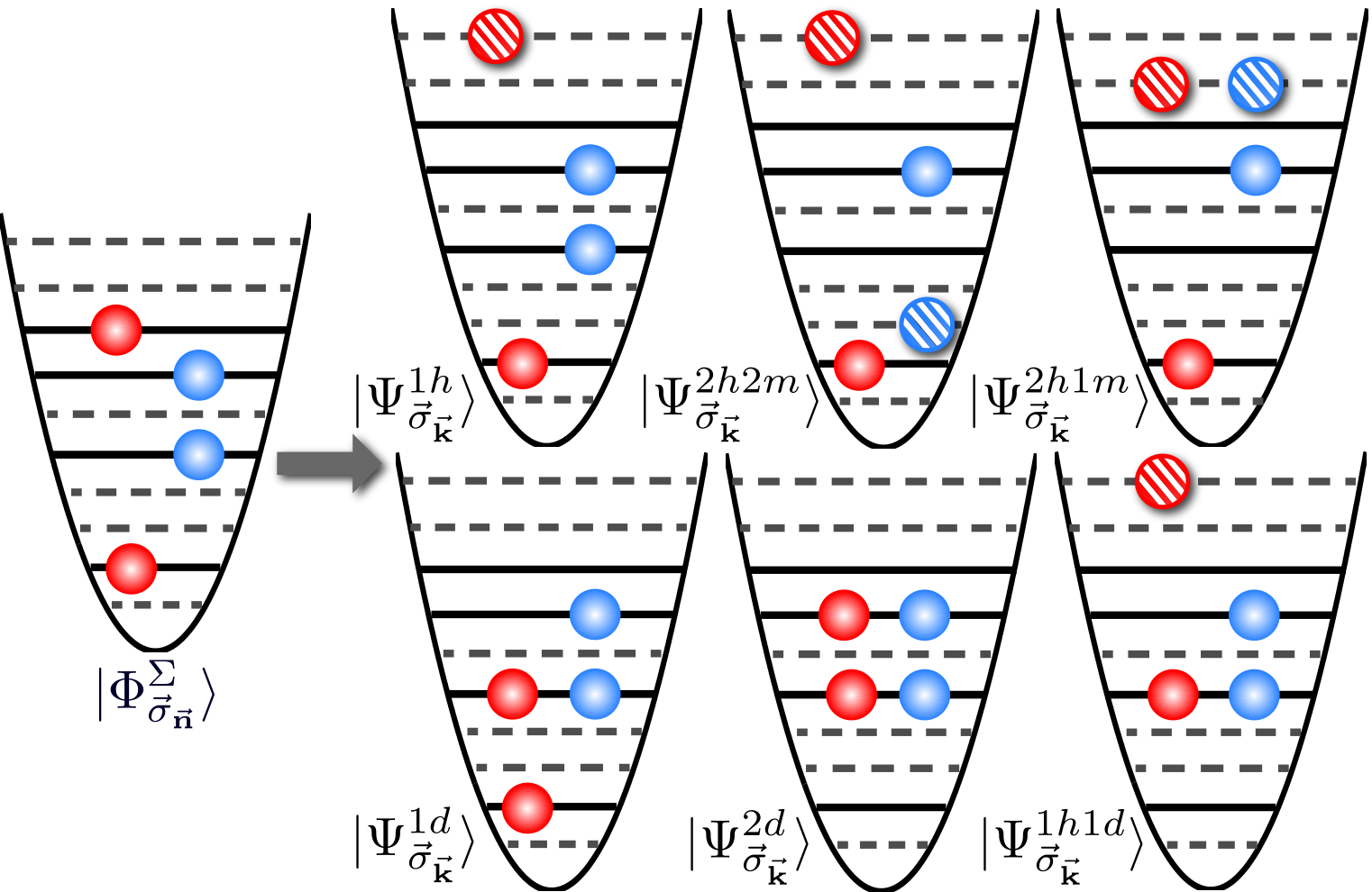
Since H^𝐧→S2{\hat{H}}^{S_{2}}_{\vec{\bf n}} acts on the Σ\Sigma subspace, it is convenient to explicitly write it in terms of spin operators. To accomplish that, we divide the states |Ψσ→𝐤→Υ⟩|\Psi^{\Upsilon}_{\vec{\bf\sigma}_{\vec{\bf k}}}\rangle into 6 different categories, |Ψσ→k→1​h⟩,|Ψσ→𝐤→2​h​2​m⟩,|Ψσ→𝐤→2​h​1​m⟩,|\Psi^{1h}_{\vec{\bf\sigma}_{\vec{k}}}\rangle,|\Psi^{2h2m}_{\vec{\bf\sigma}_{\vec{\bf k}}}\rangle,|\Psi^{2h1m}_{\vec{\bf\sigma}_{\vec{\bf k}}}\rangle, |Ψσ→𝐤→1​d⟩,|Ψσ→𝐤→2​d⟩,|Ψσ→𝐤→1​h​1​d⟩|\Psi^{1d}_{\vec{\bf\sigma}_{\vec{\bf k}}}\rangle,|\Psi^{2d}_{\vec{\bf\sigma}_{\vec{\bf k}}}\rangle,|\Psi^{1h1d}_{\vec{\bf\sigma}_{\vec{\bf k}}}\rangle, which are shown in Fig. 8.

The states labeled with superscripts 1​h1h and 2​h​2​m2h2m are states which have one and two atoms populating a mode not belonging to the initially populated 𝐧→={𝐧1,𝐧2,…,𝐧N}\vec{\bf n}=\{{\bf n}_{1},{\bf n}_{2},\dots,{\bf n}_{N}\} manifold respectively. The states labeled with superscripts 2​h​1​m2h1m are states which have two atoms both populating one mode not belonging to the initially populated manifold. The states labeled with superscripts 1​d1d and 2​d2d have one and two modes in the initially populated manifold occupied by two atoms (doublon) respectively. Finally states labeled by superscripts 1​h​1​d1h1d have one atom populating a mode outside the initially occupied manifold and a doublon. We will consider the various contributions case by case in Appendix 2. Here we only quote the final result, assuming collective interactions and dropping terms that are constants of motion.
Refer to caption
Figure 8: (Color Online) Schematic representation of the various virtual processes. Here the filled circles denote gg (blue) and ee (red) atoms in the initially populated levels (also shown with a solid line). The striped circles denote atoms virtually populating off-resonant levels, shown with a dashed line. Note that the classification is made in terms of the number of doublons or populated states outside the initially populated manifold. Processes in which, in addition to the formation of a hole or a doublon within the occupied manifold, the spin is switched between two atoms are also included in each classification but are not necessary shown in the schematics. Also, since this is a schematic plot, for simplicity, we show two ee atoms and two gg atoms only and the color was selected randomly. For example, for the cases (1h), (1d), (2d) and (1h1d) corresponding processes exist where g (blue) atoms are the ones that get excited.
H^𝐧→S2\displaystyle{\hat{H}}_{\vec{\bf n}}^{S_{2}} =\displaystyle= a1T​S^z+a2T​(S^z)2+a3T​(S^z)3,\displaystyle a^{T}_{1}{\hat{S}}^{z}+a^{T}_{2}({\hat{S}}^{z})^{2}+a^{T}_{3}({\hat{S}}^{z})^{3}, (55)

The parameters a1,2,3Ta^{T}_{1,2,3} are explicitly computed in Appendix 2.

Among those corrections, linear and quadratic contributions can be absorbed into the spin Hamiltonian, and only the processes proportional to (S^z)3({\hat{S}}^{z})^{3} give rise to an additional term. Multi-body interactions arising from virtual scattering processes have been shown to introduce measurable corrections in quantum phase revivals in the Bose-Hubbard model [58, 59]. The cubic terms can give rise to visible corrections to the Ramsey-fringe contrast as recently measured in the JILA Sr clock and reported in Ref. [22]. Here we also show, in Sec.VII.2.2, that they play an important role in the Yb Ramsey-fringe contrast decay.

In principle, terms proportional to (S^z)4({\hat{S}}^{z})^{4} could appear in the effective Hamiltonian. We find, however, that they vanish in our system due to the fact that when an atom in mode 𝐧j{\bf n}_{j} scatters to an already occupied mode, 𝐧j′{\bf n}_{j^{\prime}}, forming a doublon, the reverse process (an atom in mode 𝐧j′{\bf n}_{j^{\prime}} scatters to mode 𝐧j{\bf n}_{j} forming a doublon), contributes with the opposite sign to the effective model, and thus, both cancel.

VI Ramsey interrogation: Beyond the collective regime

Negligible excitation inhomogeneity is not necessarily a good approximation in all optical lattice clock experiments. For example, in the Yb optical lattice clock at NIST, the current operating temperature is typically around 10​μ​K10\mu K and Δ​Ω/Ω¯\Delta\Omega/\bar{\Omega} can be in some cases as high a 0.25 (see Fig. 4). In the following sections we describe various ways to treat inhomogenous excitation and interaction effects that cause population of non-collective states. We first consider the case of collective interactions, where an analytic solution to the full quantum problem in the presence of an excitation inhomogeneity can be derived based on perturbation theory in Δ​Ω/Ω¯\Delta\Omega/\bar{\Omega}. Next, we discuss a solution based on the TWA that incorporates in the model, not only excitation inhomogeneity but also inhomogeneity in the spin coupling constants and losses.

VI.1 Analytic solution

In the presence of excitation inhomogeneity, an analytic treatment based on perturbation theory can be performed under the collective Hamiltonian approximation, i.e. neglecting two body losses and assuming collective two-body interactions.

To accomplish that one writes Ω𝐧j=Ω¯𝐧→+δ​Ω𝐧j\Omega_{{\bf n}_{j}}=\bar{\Omega}_{\vec{\bf n}}+\delta\Omega_{{\bf n}_{j}}, with Ω¯𝐧→=∑jΩ𝐧j/N\bar{\Omega}_{\vec{\bf n}}=\sum_{j}\Omega_{{\bf n}_{j}}/N the mean Rabi frequency and treats δ​Ω𝐧j/Ω¯\delta\Omega_{{\bf n}_{j}}/\bar{\Omega} as a perturbation parameter. Keeping only the leading order correction, which can be shown to be quadratic in Δ​Ω𝐧→=∑jΩ𝐧𝐣2/N−Ω¯𝐧→2\Delta{\Omega}_{\vec{\bf n}}=\sqrt{\sum_{j}\Omega_{\bf n_{j}}^{2}/N-\bar{\Omega}_{\vec{\bf n}}^{2}}, i.e. the first-order corrections vanish, and after a lengthly but straightforward calculation described in Appendix 3, one can compute the number of excited atoms, Ne,𝐧→​(t1,t2)N_{e,\vec{\bf n}}(t_{1},t_{2}), in Ramsey spectroscopy. The expression is quite complicated and we do not explicitly show it in the main text. Instead here we discuss its behavior in the weakly interacting regime, χ𝐧→​τ≪1\chi_{\vec{\bf n}}\tau\ll 1 and J𝐧→⟂​τ≪1{J}^{\perp}_{\vec{{\bf n}}}\tau\ll 1, where one can show that the density shift becomes:

2​π​Δ​ν𝐧→Inh=(N−1)​[C𝐧→−χ𝐧→∗​cos⁡(θ¯1𝐧→)]−N​Δ​θ2𝐧→​Δ​θ1𝐧→​[J𝐧→⟂+χ𝐧→N​sin2⁡(θ¯1𝐧→)]​(cot⁡(θ¯2𝐧→)sin⁡(θ¯1𝐧→)),\displaystyle 2\pi\Delta\nu_{\vec{{\bf n}}}^{{\rm Inh}}=(N-1)\Big[{C}_{\vec{{\bf n}}}-{\chi}^{*}_{\vec{{\bf n}}}\cos({\bar{\theta}}_{1}^{\vec{\bf n}})\Big]-N\Delta\theta_{2}^{\vec{\bf n}}\Delta\theta_{1}^{\vec{\bf n}}\left[{J}^{\perp}_{\vec{{\bf n}}}+\frac{\chi_{\vec{{\bf n}}}}{N}\sin^{2}({\bar{\theta}}_{1}^{\vec{\bf n}})\right]\left(\frac{\cot({\bar{\theta}}_{2}^{\vec{\bf n}})}{\sin({\bar{\theta}}_{1}^{\vec{\bf n}})}\right), (56)
χ𝐧→∗=χ𝐧→​[1+(N−3)2​(N−1)​(Δ​θ1𝐧→)2],\displaystyle{\chi}^{*}_{\vec{{\bf n}}}=\chi_{\vec{{\bf n}}}\left[1+\frac{(N-3)}{2(N-1)}(\Delta\theta_{1}^{\vec{\bf n}})^{2}\right], (57)

with Δ​θ1,2𝐧→=Δ​Ω𝐧→​t1,2\Delta\theta_{1,2}^{\vec{\bf n}}=\Delta{\Omega}_{\vec{\bf n}}t_{1,2} and θ¯1,2=Ω¯𝐧→​t1,2\bar{\theta}_{1,2}=\bar{\Omega}_{\vec{\bf n}}t_{1,2}.

The expression of the shift in the weakly interacting limit is very illuminating. Note that while to leading order (Δ​θ=0\Delta\theta=0) the density shift is only determined by the excitation fraction, cos⁡(θ¯1)=(Ng−Ne)/2\cos({\bar{\theta}}_{1})=(N_{g}-N_{e})/2, and is independent of the second pulse area, θ¯2{\bar{\theta}}_{2}, excitation inhomogeneity does introduce a dependence of the density shift on the second pulse area. An intuitive explanation for that can be obtained by noticing that the density shift is extracted from a collective measurement. Therefore, if there are atoms excited outside the symmetric Dicke manifold due to the first pulse, they only contribute to the measured signal if they are brought back to the symmetric Dicke manifold by the second pulse. The mean-field expression, Eq. (56), also tells us that terms proportional to (Δ​θ1𝐧→)2(\Delta\theta_{1}^{\vec{\bf n}})^{2} just slightly renormalize the overall magnitude of the density shift, χ𝐧→→χ𝐧→∗\chi_{\vec{\bf n}}\to\chi^{*}_{\vec{\bf n}}, without affecting its general dependence on the excitation fraction. On the other hand, the term proportional to Δ​θ1𝐧→​Δ​θ2𝐧→\Delta\theta_{1}^{\vec{\bf n}}\Delta\theta_{2}^{\vec{\bf n}} does modify the dependence of the density shift on pulse area and vanishes at θ¯2𝐧→=π/2{\bar{\theta}}_{2}^{\vec{\bf n}}=\pi/2.

Outside the weakly interacting regime, the assumption that the density shift scales mostly linearly with the particle number breaks down. One important consequence of this observation is that the behavior of the N=NTN=N_{T} particle system cannot be reproduced by solving the N=2N=2 system and then rescaling the interactions, as claimed in Ref. [17], i.e. replacing χ𝐧→\chi_{\vec{\bf n}} and J𝐧→⟂{J}^{\perp}_{\vec{\bf n}} in the N=2N=2 solutions by χ𝐧→eff→χ𝐧→​(NT−1){\chi}_{\vec{\bf n}}^{\rm eff}\to\chi_{\vec{\bf n}}(N_{T}-1) and J𝐧→⟂eff→J𝐧→⟂​NT/2{{J}^{\perp}_{\vec{\bf n}}}^{\rm eff}\to{{J}^{\perp}_{\vec{\bf n}}}N_{T}/2. The relevant role of non-linear effects is illustrated in Fig. 9. In the top panel we compare the behavior of three systems with different N=2,6,12N=2,6,12. We fix the interactions such that χ𝐧→​(N−1){\chi}_{\vec{\bf n}}(N-1) are all equal as well as all J𝐧→⟂​N{{J}^{\perp}_{\vec{\bf n}}}N. While the curves N=6N=6 and 1212 are very close to each other, they do not agree with the N=2N=2 solution.

Note also that for the many-body system, N≫2N\gg 2, the part of the shift sensitive to the second pulse area is mainly proportional to N⁡(J𝐧→⟂)N({J}^{\perp}_{\vec{\bf n}}) (up to 1/N1/N corrections) and not to 2​J𝐧→⟂+χ𝐧→​sin2⁡(θ¯1)2{J}^{\perp}_{\vec{\bf n}}+\chi_{\vec{\bf n}}\sin^{2}({\bar{\theta}}_{1}), as it is the case for N=2N=2. This phenomenon is visible in the bottom panel of Fig. 9, which shows the shift vs excitation fraction for three different second pulse areas: (0.25,0.5CLOSE(0.25,0.5, and OPEN0.75)​π0.75)\pi. At J⟂=0{{J}^{\perp}}=0 and θ¯1𝐧→=π/2\bar{\theta}_{1}^{\vec{\bf n}}=\pi/2 (close to zero crossing for the parameters used in the plot) the density shift only exhibits a significant dependence on the second pulse area when N=2N=2.

Figure 9: (Color Online) Shift vs excitation fraction for different atom numbers: N=2N=2 (Black open squares), 66 (no symbol), and 1212 (red circles). The convention for the second pulse area is: θ¯2𝐧→\bar{\theta}_{2}^{\vec{\bf n}}: 0.25​π0.25\pi (solid), 0.5​π0.5\pi (dashed line) and 0.75​π0.75\pi (short-dashed line). We set C𝐧→=0C_{\vec{\bf n}}=0. The values of the other interactions were chosen such that χ𝐧→​(N−1)\chi_{\vec{\bf n}}(N-1) are all equal as well as J𝐧→⟂​N{J}^{\perp}_{\vec{\bf n}}N. For N=2N=2, we set χ𝐧→=1{\chi}_{\vec{\bf n}}=1 and J𝐧→⟂=0{{J}^{\perp}_{\vec{\bf n}}}=0 and −0.6-0.6, for the top and bottom panels respectively. Note that for N>2N>2 and J𝐧→⟂=0{J}^{\perp}_{\vec{\bf n}}=0, the density shift is quite insensitive to the second pulse area as predicted by theory.

VI.2 TWA and Mean-field solutions

We will now use the TWA to go beyond the collective approximation that was required to derive the equations of motion in prior sections. The TWA allows us to include different types of mechanisms, which bring the system out of the collective Dicke manifold, such as single-particle excitation inhomogeneities and non-collective elastic and inelastic two-body collisions. We can also easily include one-body losses due to, for example, background gas collisions. The latter are characterized by the jump operators Γj​α​c^𝐧j​α\sqrt{\Gamma_{j\alpha}}\hat{c}_{{\bf n}_{j}\alpha}, which annihilate the atom jj in spin state α\alpha.

For the mean-field treatment, we assume the reduced density matrix of the many-body system factorizes as described in Eq. (47). With the aim of dealing with long-range interactions, it is better to write the equations of motion of the Fourier transformed quantities:

ρα​α​(k)\displaystyle\rho_{\alpha\alpha}(k) =\displaystyle= ∑j=1Nei​2​π​j​kN​ρ~α,αj\displaystyle\sum_{j=1}^{N}e^{i\frac{2\pi jk}{N}}\tilde{\rho}^{j}_{\alpha,\alpha} (58)
ρe​g​(k)\displaystyle\rho_{eg}(k) =\displaystyle= ∑j=1Ne−i​2​π​j​kN​ρ~e,gj=ρg​e∗​(k)\displaystyle\sum_{j=1}^{N}e^{-i\frac{2\pi jk}{N}}\tilde{\rho}^{j}_{e,g}=\rho_{ge}^{*}(k) (59)

The equations of motion derived in this way are general, and in section VII, will be applied to model the Yb clock dynamics. These equations reduce to Eqs. (49-51) when the interaction parameters are collective, i.e. have only k=k′=0k=k^{\prime}=0 components. In their most general form, the equations of motion are nontrivial, and we present them in Appendix 4. Here instead we proceed to analyze simpler relevant cases, which will allow us to test the validity of their corresponding TWA dynamics (obtained after sampling the solutions of the mean-field equations with the Wigner distribution). We proceed by considering two cases, one in which the inhomogeneity is caused by interactions and the other in which it is caused by single-particle terms. Since analytic solutions are only available when one restricts the dynamics to a pure Hamiltonian evolution, in the reminder of this section we will neglect single-particle and two-body losses.

VI.2.1 Non-collective interactions

∙\bullet Ising Case

Figure 10: (Color Online) Ramsey-fringe-contrast decay for the case of power-law Ising interactions in a 2D square array composed of 121 atoms (See text). The first pulse is set to π/2\pi/2. The solid lines correspond to the exact solution obtained from Ref. [52]. The dashed lines are the TWA solution. From top to bottom the curves correspond to α=1,0.5\alpha=1,0.5, and 0.20.2.
Figure 11: (Color online) Top panels: Comparisons of the density shift vs excitation fraction predicted by the collective TWA and the generic TWA at τ=50\tau=50 ms. The generic TWA accounts for the mode dependence of pp-wave interactions. Here zero excitation inhomogeneity is assumed (Δ​Ω=0\Delta\Omega=0). A thermal average over initially populated modes is performed. The left panel is for a fixed number of atoms, N=20N=20. In the right panel, we have done an average over the atom number in the pancakes using a Poissonian distribution with N¯∼9\bar{N}\sim 9 (see Sec. VII.1). Here ve​e=vg​gv^{ee}=v^{gg}, thus C𝐧j,𝐧j′=0C_{{\bf n}_{j},{\bf n}_{j^{\prime}}}=0. Bottom panels: Comparison of the contrast decay vs time predicted by the collective TWA and generic TWA for different first pulse areas (indicated in the plot). Again, the left panels is for a fixed number of atoms, N=20N=20, and the right panel is computed after performing an atom number average.

The Ising case corresponds to J𝐧j,𝐧j′⟂=0{J}^{\perp}_{{\bf n}_{j},{\bf n}_{j^{\prime}}}=0. An exact solution for the Ising dynamics exists for an initial product state and for arbitrary spin coupling constants [52, 60, 31, 61, 62]. This analytic solution allows us to benchmark the validity of the TWA beyond the collective regime, assuming zero transverse interactions J𝐧j,𝐧j′⟂=0{J}^{\perp}_{{\bf n}_{j},{\bf n}_{j^{\prime}}}=0 and no losses. We will also assume, for simplicity, no excitation inhomogeneity during pulses. In this case, at the mean-field level, one obtains:

ρe​g​(k=0,τ)=(S0x+i​S0y)​exp⁡[−i​τ​ℳo]0,0,\displaystyle{\rho_{eg}(k=0,\tau)}=(S^{x}_{0}+{\rm i}S^{y}_{0})\exp[-{\rm i}\tau\mathcal{M}^{o}]_{0,0}, (60)

with

ℳk,k′o\displaystyle\mathcal{M}^{o}_{k,k^{\prime}} ≡\displaystyle\equiv δ​Ik,k′−2​S^0z​χk′−k,0−N​Ck′−k,0,\displaystyle\delta I_{k,k^{\prime}}-2{\hat{S}}^{z}_{0}\chi_{k^{\prime}-k,0}-NC_{k^{\prime}-k,0}, (61)
χk,0\displaystyle\chi_{k,0} ≡\displaystyle\equiv 1N2​∑j,j′=1Nei​2​π​j​kN​χ𝐧→j,𝐧→j′,\displaystyle\frac{1}{N^{2}}\sum_{j,j^{\prime}=1}^{N}e^{i\frac{2\pi jk}{N}}\chi_{\vec{\bf n}_{j},\vec{\bf n}_{j^{\prime}}}, (62)
Ck,0\displaystyle C_{k,0} ≡\displaystyle\equiv 1N2​∑j,j′=1Nei​2​π​j​kN​C𝐧→j,𝐧→j′.\displaystyle\frac{1}{N^{2}}\sum_{j,j^{\prime}=1}^{N}e^{i\frac{2\pi jk}{N}}C_{\vec{\bf n}_{j},\vec{\bf n}_{j^{\prime}}}. (63)

Here II is the identity matrix. {S0x,S0y,S0z}\{S^{x}_{0},S^{y}_{0},S^{z}_{0}\} are the components of the collective Bloch vector after the first pulse. In Fig. 10, we show the comparisons for a system of N=121=11×11N=121=11\times 11 atoms assuming that modes 𝐧→\vec{\bf n} form a 2D square lattice array. We set χ𝐧→j,𝐧→j′∝1/|𝐧j−𝐧j′|α\chi_{\vec{\bf n}_{j},\vec{\bf n}_{j^{\prime}}}\propto 1/|{\bf n}_{j}-{\bf n}_{j^{\prime}}|^{\alpha} and vary α=0.2,0.5,1\alpha=0.2,0.5,1. Note this choice of χ𝐧→j,𝐧→j′\chi_{\vec{\bf n}_{j},\vec{\bf n}_{j^{\prime}}} is done just for convenience without any direct link with the mode dependence of χ𝐧→j,𝐧→j′\chi_{\vec{\bf n}_{j},\vec{\bf n}_{j^{\prime}}} when it describes actual ss or pp- wave interactions. The physically relevant case for the clock will be described below. For α=0.2,0.5\alpha=0.2,0.5, the exact and TWA solutions agree well. However, for α=1\alpha=1, deviations start to become important. An approximate criterion for the validity of the TWA for a translationally invariant system is that, if one defines [31] Ξm=∑jχ𝐧→0,𝐧→jm\Xi_{m}=\sum_{j}\chi_{\vec{\bf n}_{0},\vec{\bf n}_{j}}^{m}, then Ξ12≈N​Ξ2\Xi_{1}^{2}\approx N\Xi_{2}. Note that, in this analysis, we have not added any quantum vacuum noise to the initially empty k≠0k\neq 0 modes. However, we have confirmed that its addition only slightly changes the conclusions.

∙\bullet Pure pp-wave interactions

We now take advantage of the TWA to benchmark the validity of the collective model when the interaction inhomogeneity comes from the mode dependence of the pp-wave interactions. In this case, for simplicity we also assume no excitation inhomogeneity during the pulses and assume no single particle or two-body losses. We also set ss-wave interactions to zero and perform a thermal average over populated modes assuming a Boltzmann distribution (see Sec. VII.1). In Fig. 11, we show the density shift and the Ramsey fringe contrast decay predicted by the TWA solution, both with and without interaction inhomogeneity. While the density shift agrees fairly well between the collective and non-collective solutions, the contrast shown for the high (θ1=0.8​π\theta_{1}=0.8\pi) initial pulse area has a slower decay for the case of collective interactions. On the contrary, at initial pulse areas close to π/2\pi/2, the agreement between the two solutions is fair, and the collective model exhibits just a slightly faster decay of the contrast. The disagreement of the contrast at high excitation fraction is because, at these conditions (a similar effect happens at small tipping angles), the contrast reduction comes primarily from simple dephasing due to the different precession rates of the Bloch vector for different realizations of the interaction parameters. Recall that the dynamics induced by mean-field interactions correspond to a precession around an effective magnetic field whose strength depends on atom number, interaction strength, and excitation fraction, Eq. (39). For the collective model that type of dephasing is much weaker. On the contrary, if C𝐧→j,𝐧→j′=0C_{\vec{\bf n}_{j},\vec{\bf n}_{j^{\prime}}}=0, as it is in this example, the effective magnetic field vanishes at θ1=π/2\theta_{1}=\pi/2. Thus, for θ1\theta_{1} close to π/2\pi/2, dephasing is minimal and contrast decay is dominated by many-body effects, which are fairly well-captured by the collective model.

Refer to caption
Figure 12: (Color online) Left panel: Comparison of the density shift vs excitation fraction predicted by the analytic perturbative treatment (solid blue line), the TWA (filled blue dots) and the mean-field (red squares) with excitation inhomogeneity. We assumed collective interactions, set Δ​Ω/Ω¯=0.25\Delta\Omega/\bar{\Omega}=0.25 and fixed N=30N=30. The density shift is computed at χ𝐧→​τ=0.04\chi_{\vec{\bf n}}\tau=0.04. Here ve​e=vg​gv^{ee}=v^{gg}, thus C𝐧→=0C_{\vec{\bf n}}=0. Right panel: Ramsey contrast decay vs time including excitation inhomogeneity predicted by the analytic perturbative treatment (solid blue line), the TWA (filled blue dots), and the mean-field (red squares). The pulse area is set to π/2\pi/2.

Despite the disagreement of the contrast at low/high excitation fractions and at zero ss-wave interactions, the collective model remains very useful for describing experimental observations during the interrogation of the clock. The reason is that, instead of a single pancake with fixed atom number, in the experiment, there is an array of pancakes populated with a Poissonian distribution (as explained below). If one takes into account the Poissonian average, one recovers a good agreement between the collective and non-collective models even at low/high excitation fractions, as shown in Fig. 11. In this case, dephasing due to the different atom number in each lattice pancake dominates the contrast decay at low/high excitation fractions. When the Poissonian average is included, the cases with low/high pulse areas are the ones that exhibit the fastest Ramsey fringe contrast decay. Note that, for Fig. 11, the mean-atom number per the pancake used for the plots with a Poissonian distribution was N¯∼9\bar{N}\sim 9. On the contrary, for the fixed-atom-number plots we set N=20N=20. The difference in atom number is the only reason why the overall timescale for the contrast decay in the Poissonian-averaged plots is slower than in the fixed-atom-number ones.

We also expect that finite |J𝐧→j,𝐧→j′⟂|>0|J^{\perp}_{\vec{\bf n}_{j},\vec{\bf n}_{j^{\prime}}}|>0 interactions (induced by ss-wave collisions) will enhance the gap between the collective Dicke manifold, S=N/2S=N/2, and the other manifolds. A larger gap will further suppress population leakage outside the former (gap protection)[48] and will improve the collective approximation. The validity of the gap protection idea is explicitly shown in Appendix 5, where we use a box potential instead of a harmonic potential to make the mode dependence of the pp-wave interactions even stronger. There we show that the dynamics converge to the collective dynamics as the mean value of |J𝐧→j,𝐧→j′⟂||J^{\perp}_{\vec{\bf n}_{j},\vec{\bf n}_{j^{\prime}}}| is increased.

VI.2.2 Excitation induced inhomogeneity

In the presence of finite φ\varphi, Eq. (6), the gap protection does not help to prevent leakage of population outside the Dicke manifold. This is because the transfer is made during short pulses where interactions play no role and single-particle excitation inhomogeneity is the leading transfer mechanism. In Fig. 12, we compare the analytic solution found in Sec. VI.1 using perturbation theory in Δ​Ω/Ω¯\Delta\Omega/\bar{\Omega} (solid blue line), the TWA (filled blue circles), and a pure mean-field with excitation inhomogeneity (red squares). Fig. 12 assumes collective interactions and equal first and second pulse areas. For comparison purposes, we also show the analytic solution for the density shift in the case of zero inhomogeneity (dashed purple line). Note that excitation inhomogeneity manifests itself in the density shift mainly at high excitation fractions where it gives rise to some curvature. The figure also shows that the density shift is well captured by both the TWA and the mean-field. On the contrary, the Ramsey fringe contrast decay is only captured by the TWA and analytic solutions, which agree well with each other. The mean-field does not predict any contrast decay. The pulse area for the Ramsey fringe contrast shown in Fig. 12 was set to be π/2\pi/2 .

VII Comparisons with optical lattice clock experiments

After developing and benchmarking in great detail the theoretical formalism, we now proceed to apply it to describe experimental measurements performed in the 87Sr JILA optical lattice clock [11, 22] and in the NIST 171Yb [19, 20] optical lattice clock. One of the main differences between the two clocks is their temperature. While the JILA clock operates typically at temperatures between (1−4)​μ(1-4)\muK and with a typical excitation inhomogeneity Δ​Ω/Ω¯≲0.1\Delta\Omega/\bar{\Omega}\lesssim 0.1, the 171Yb clock typically operates at temperatures at or somewhat above 10​μ10\muK with corresponding excitation inhomogeneity Δ​Ω/Ω¯∼0.25−0.3\Delta\Omega/\bar{\Omega}\sim 0.25-0.3. These differences have significant consequences for the proper theory model required to describe the experiment. While the pure collective model is sufficient to describe the many-body dynamics in the 87Sr clock, as explicitly shown below, the inclusion of excitation inhomogeneity is needed to reproduce the 171Yb measurements. We first start by describing in more detail the experimental set-up, which is common for the two clocks, and then present the experimental measurements and comparisons with theory.

VII.1 Spatial averaging and finite temperature

In the experiments, a one dimensional lattice is used to confine the atoms creating an array of 2D disk-shaped arrays or pancakes (see Fig. 2b). The atom number distribution along the array is determined by assuming the atoms are loaded in the MOT (magneto-optical trap) with a Gaussian density profile, and that this profile is kept the same but simply partitioned into lattice sites when the 1D lattice is turned on. In this case ρ(l)=NT​aσM​2​πe−(la)2/(2σM2)\rho(l)=\frac{N_{T}a}{\sigma_{M}\sqrt{2\pi}}e^{-(la)^{2}/(2\sigma_{M}^{2})} is taken as the density at pancake ll after integrating along the other two directions. Here σM\sigma_{M} is the 1/e1/e MOT radius, which is ∼30​μ\sim 30\mum for 87Sr clock and ∼130​μ\sim 130\mum for the 171Yb clock, a∼0.4a\sim 0.4 μ\mum is the lattice spacing (approximately the same for both experiments) and NTN_{T} the total atom number. The atom number fluctuates from realization to realization according to a Poissonian distribution, and the probability of having N>0N>0 atoms at lattice site ll is ℛ⁡(l,N)=A​e−ρ⁡(l)​ρ​(l)NN!{\mathcal{R}}(l,N)=Ae^{-\rho(l)}\frac{\rho(l)^{N}}{N!} with AA a normalization constant. Any experimental observable should be then calculated as 𝒪Exp=∑N𝒪⁡(N)​ℛ​(N)\mathcal{O}_{\rm{Exp}}=\sum_{N}\mathcal{O}(N){\mathcal{R}}(N) with ℛ⁡(N)=∑lℛ⁡(l,N){\mathcal{R}}(N)=\sum_{l}{\mathcal{R}}(l,N). In Fig. 13, we show an atom number distribution for a typical number of NT∼26000N_{T}\sim 26000 atoms in the Yb clock. The Sr clock operates with a smaller atom number, NT=5000N_{T}=5000, but, due to different trapping conditions, the average distribution of atoms in both experiments is similar, as can be seen in Fig. 13.

Figure 13: (Color Online) Atom number distribution: The solid blue distribution is for the Yb 1D optical lattice clock at a typical atom number NT=26000N_{T}=26000; the dashed purple distribution is for the Sr 1D optical lattice clock at typical atom number NT=5000N_{T}=5000.

In most of the calculations performed above, we fixed the set of vibrational modes to be 𝐧→\vec{\bf{n}}. However, to compare with experiments, we need to perform a thermal average. For μ\muK temperatures, at which the clocks operate, we can assume the modes are initially populated according to a Maxwell-Boltzmann distribution, computed using single-particle energies. Although so far we have assumed that atoms are frozen along the axial direction, this assumption is not fully correct for the Yb lattice clock operated at ∼10​μ\sim 10\muK with a typical axial trapping frequency of νZ=75−80\nu_{Z}=75-80 KHz. In this case, the mean axial mode occupation number n¯Z∼2.5\bar{n}_{Z}\sim 2.5, and to compare with the Yb experiment, we perform a thermal average over excited-optical-lattice bands.

Figure 14: (Color Online) Density shift in Ramsey spectroscopy vs excitation fractions measured in the Sr clock: The filled symbols show experimental data. The dashed(blue) line is the prediction from the collective TWA model and the solid (green) line the collective mean-field model. The experimental data was normalized to a typical time-averaged total atom number of 1000 atoms. The excitation fraction was also time-averaged. See Ref. [22] and text for more information.
Figure 15: (Color Online) Atom number decay and Ramsey fringe contrast vs dark time measured in the Sr clock: The filled symbols show experimental data, the solid lines are the predictions from the collective TWA model, and the dashed lines are the predictions from the collective mean-field model. See text for more information. An overall scaling factor on the order of ∼0.9−1\sim 0.9-1 in the contrast plots, that accounted for the experimental dead-time between the end of the second pulse and the population measurements was used in the theory curves to match the contrast at zero dark time. Statistical error bars for experimental data are comparable to symbol’s size. See also Ref. [22].

VII.2 Ramsey Spectroscopy

The experiments performed Ramsey spectroscopy measurements and varied the atom number, pulse area, and the initial state of the atoms. The results are summarized in Figs. 14-16 for the Sr clock and Figs. 17-18 for the Yb clock. In those plots, the theoretical predictions are also shown.

VII.2.1 Sr optical lattice clock

Let us first discuss the Sr clock, which admits a simpler theoretical treatment based on a pure collective model. Figure 14 shows the measured density shift vs excitation fraction. The excitation fraction was changed by varying the first pulse area. In the presence of two-body losses, the excitation fraction is not constant during the dark time, and, to simplify the comparisons with theory, a time-averaged excitation fraction was used for the density shift plot. The latter was extracted in the experiment by performing a set of independent measurements periodically inserted into the clock sequence [22]. The duration of the dark time, τ\tau, was set to 80 ms, and the final pulse area to π/2\pi/2. The typical axial and radial sample temperature, measured by sideband spectroscopy and Doppler spectroscopy respectively, were between, TZ∼1−2​μT_{Z}\sim 1-2\muK and TR∼2−4​μT_{R}\sim 2-4\muK; the trapping frequencies were set to νZ=80\nu_{Z}=80 kHz and νR∼450\nu_{R}\sim 450 Hz; and the typical misalignment angles were small enough that excitation inhomogeneity was negligible. Under these operating conditions, the collective model, after performing an average over the atom number distribution, is expected to work fairly well. This expectation is confirmed by the linear dependence of the shift at high excitation fraction and the good agrement between the collective TWA predictions and the experimental data. Since only the gg interaction parameters are known, bg​g∼76b_{gg}\sim 76 aBa_{B} (aBa_{B} the Bohr radius)[11], we used the density shift data to determine the parameters Ve,g−Vg,g=−2π×0.27V^{e,g}-V^{g,g}=-2\pi\times 0.27 Hz and Ve,e−Vg,g=0.4​Ve,gV^{e,e}-V^{g,g}=0.4V^{e,g}. Note that these parameters are almost temperature independent.

Figure 15 shows the atom number decay and the normalized Ramsey fringe contrast. By normalized we mean that the contrast was rescaled by the corresponding atom number at a given time. In the experiment, the Ramsey fringe contrast was extracted in a manner that is insensitive to the frequency noise of the local oscillator. For details, see Ref. [22, 23]. Four different first pulse areas were used (the second pulse area was always π/2\pi/2) and are indicated with different symbols in the figure. The Ramsey pulses were always shorter than 66 ms. Atom number decay data was used to determine Γe,e=2​π×0.1\Gamma^{e,e}=2\pi\times 0.1 Hz. Γe,g\Gamma^{e,g} was consistent with zero in agreement with measurements reported in Ref. [21]. There the single atom decay rates were also measured to be Γe∼Γg=2​π×0.01\Gamma^{e}\sim\Gamma^{g}=2\pi\times 0.01 Hz, and we used those values. These parameters together with the values of Ve,g−Vg,gV^{e,g}-V^{g,g} and Ve,e−Vg,gV^{e,e}-V^{g,g} extracted from the density shift were used to compute the Ramsey contrast decay curves.

We added a cubic term to account for the virtual populations of the off-resonant modes as explained in Sec.V. Since the coupling constants a1,2,3Ta_{1,2,3}^{T} cannot be trivially computed, we used instead the quantities χP​P(3,6)\chi^{(3,6)}_{PP} – which give rise to the relevant cubic contributions – as fitting parameters (see Appendix 2) and set ae​g−=0a_{eg}^{-}=0. The values of χP​P(3,6)\chi^{(3,6)}_{PP} utilized generated an additional term ∑r=03Ar​(N^e)3−r​(N^g)r\sum_{r=0}^{3}A_{r}(\hat{N}_{e})^{3-r}(\hat{N}_{g})^{r} with A0=2​π×0.0016A_{0}=2\pi\times 0.0016 Hz, A1=−2π×0.0058A_{1}=-2\pi\times 0.0058 Hz, A2=2​π×0.003A_{2}=2\pi\times 0.003 Hz, A3=2​π×0.0011A_{3}=2\pi\times 0.0011 Hz. Although the cubic corrections are small and played no role in the density shift, they improved the agreement between theory and experiment. To emphasize this point in Fig. 16, we explicitly compare the theory predictions of the contrast with and without cubic terms.

In addition to the collective TWA solutions, we also show the collective mean-field predictions. Both were computed after performing an average over the atom number distribution. Excellent agreement is observed between the collective TWA and the experimental data 22 2 In Figs. 14, in contrast to the theory presented in Ref. [22] where losses were neglected, we do include losses and perform a time average.. The mean-field model reproduces the density shift measurements and is able to capture the fast contrast decay at low excitation fractions due to the dephasing induced by the different precession rates of the Bloch vector across different pancakes. Remember that the effective magnetic field induced by interactions is directly proportional to the density shift and depends on the pulse area and atom number. At low excitation fraction the effective magnetic field (density shift) is maximum as shown in Fig. 14. On the contrary, for the intermediate excitation fraction data points, the mean-field solution fails to reproduce the contrast decay observed experimentally. At those excitation fractions, the effective magnetic field (density shift) is almost zero –see Fig. 14 – and the contrast decay is dominated by many-body correlations not included in the mean-field model.

Figure 16: (Color Online) Ramsey contrast decay obtained from the the collective TWA with cubic terms (solid lines) and without them (dashed lines). The symbols are experimental data taken at different first pulse areas. Statistical error bars for experimental data are comparable to symbol’s size. See also Ref. [22].
Figure 17: (Color Online) Density Shift vs excitation fractions measured in the Yb clock: The filled symbols show experimental data and the open symbols joined by dashed lines show predictions from the non-collective TWA model (left) and the non-collective mean- field model (right). The blue circles and red squares were taken using a vertical and horizontal 1D lattice, respectively, and used a g→eg\to e interrogation. The yellow diamonds used a vertical lattice but interrogated the e→ge\to g transition. The experimental data measured the shift by normalizing it to a typical time-averaged total atom number of ⟨NT⟩τ=25000\langle N_{T}\rangle_{\tau}=25000 atoms. The excitation fraction was also time-averaged. See text for more information.
Figure 18: (Color Online) Atom number and Ramsey fringe contrast vs dark time measured in the Yb clock: The filled symbols show experimental data, the solid lines are the predictions from the non-collective TWA model, and the dashed lines are the predictions from the non-collective mean-field model. See text for more information. To account for the additional 25 ms dead-time between the end of the second pulse and the population measurements, we introduced an overall scaling factor ∼0.8−0.9\sim 0.8-0.9 to match the experimentally measured contrast at zero dark time. Experimental error bars are comparable to symbol’s size.

VII.2.2 Yb optical lattice clock

Now we proceed to discuss the Yb clock experiment. Figure 17 shows the measured density shift vs excitation fraction seen in the Yb clock [19, 20]. Two types of initial conditions were considered. For the red and blue points, initially all atoms were prepared in the gg state and then optically excited to the ee state. The blue data (solid circles) was taken using a vertical optical lattice and the red data (solid squares) using an horizontal optical lattice. In the vertical lattice, tunneling between neighboring lattice sites is expected to be substantially suppressed by gravity [64, 19]. That suppression is not present in the horizontal setup. Based on that and the fact that there is no substantial difference between the two sets of data, we conclude that, at least for the density shift, tunneling can be neglected. The yellow solid diamonds show the density shift measured for the initial condition, in which all the atoms were prepared in the ee state and then optically deexcited to the gg state. For all the cases, the Ramsey pulse time was t1=t2=1t_{1}=t_{2}=1 ms, the dark time was τ=80\tau=80 ms, the temperature was T=10​μT=10\mu K, the trapping frequencies were νZ=75\nu_{Z}=75 kHz and νR∼500\nu_{R}\sim 500 Hz and Δ​Ω/Ω¯∼0.25\Delta\Omega/\bar{\Omega}\sim 0.25. In 171Yb, both e−ee-e and e−ge-g losses, as well as single particle ee and gg losses, play a non-negligible role in the quantum dynamics [20]. Consequently, both the excitation fraction and atom number vary with time during the spectroscopy. The data presented here accounts for those effects by using time-averaged excitation fraction and a density shift normalized to a time-averaged atom number. The different behavior observed between the e−ge-g and g−eg-e interrogation measurements is mainly due to excitation inhomogeneity, which depends on pulse area.

Figure 18 shows the atom number decay and normalized Ramsey fringe contrast. Three different pulse areas were used (both the first and second pulse areas were the same) as indicated with different symbols in the figure. For each pulse area, two measurements were done, one at a high and the other at a low atom number. These measurements were carried out at similar but slightly different trapping conditions and temperature as compared to the ones used for the density shift: νZ=80\nu_{Z}=80 kHz, νR∼550\nu_{R}\sim 550 Hz, T≳10​μT\gtrsim 10\muK, and t1=t2=5t_{1}=t_{2}=5 ms.

The most general TWA, which accounts for excitation inhomogeneity, non-collective interactions, two-body and single-particle losses, as well as interaction effects and virtual population of motional states (cubic terms in the spin Hamiltonian), was used to model the experiment. Both a thermal average and an average over the atom number distribution in the pancakes were performed. We also compared the predictions of the pure mean-field model, which accounts for similar types of effects but without performing the sampling over the Wigner distribution. Only the gg interaction parameters are known in Yb as well, bg​g≈0b_{gg}\approx 0, and thus we used ve,e,ve,g,γe,e,ue​g,χP​P(3,6)v^{e,e},v^{e,g},\gamma^{e,e},u_{eg},\chi^{(3,6)}_{PP} (see Appendix 2) as fitting parameters. Note that, since we are not using the collective model, we quote the vα,βv^{\alpha,\beta} values and not the Vα,βV^{\alpha,\beta} values. The cubic Hamiltonian was the only term projected onto the collective manifold and included as a term P¯​∑r=03ar​[N^e3−r​(k=0)​N^gr​(k=0)]\bar{P}\sum_{r=0}^{3}a_{r}[\hat{N}_{e}^{3-r}(k=0)\hat{N}_{g}^{r}(k=0)]. Here P¯=1/N2∑j,j′P𝐧j,𝐧j′\bar{P}=1/N^{2}\sum_{j,j^{\prime}}P_{{\bf n}_{j},{\bf n}_{j^{\prime}}}. ara_{r} are functions of χP​P(6),χP​P(3)\chi^{(6)}_{PP},\chi^{(3)}_{PP}. From Ref. [20], we set γe,g=3​γe,e/5\gamma^{e,g}=3\gamma^{e,e}/5 and Γe∼Γg=2​π×0.3\Gamma^{e}\sim\Gamma^{g}=2\pi\times 0.3 Hz. The theoretical curves shown in Figs. 17 and 18 used the following set of parameters: ve,g=−2π×3.8v^{e,g}=-2\pi\times 3.8 Hz, ve,e=−0.2​ve,gv^{e,e}=-0.2v^{e,g},γe,e=2​π×2.8\gamma^{e,e}=2\pi\times 2.8 Hz, ue​g=0u_{eg}=0, a0=a3=2​π×0.3a_{0}=a_{3}=2\pi\times 0.3 Hz and a1=a3/2=−2a0/3a_{1}=a_{3}/2=-2a_{0}/3. For the Ramsey contrast measurements, we found that the 55 ms pulses used in the Yb experiment were not short enough to make interaction effects negligible during the pulses, and, because of that, we included interactions during those in the numerical simulations. We added in addition a single-particle dephasing term acting on ρe​g\rho_{eg} in all cases, e−γd​p​τe^{-\gamma_{dp}\tau} with γd​p=2\gamma_{dp}=2 Hz to capture the contrast decay observed for the low density data since, at those densities, interactions effects could not be the cause of contrast decay.

While there is a substantial number of fitting parameters, there is also a variety of experimental data curves. Note also that γe,e\gamma^{e,e} is uniquely determined by the atom loss curves and the ratio ve,e/ve,gv^{e,e}/v^{e,g} by the density shift measurements. In the Sr experiment, the collective model based on the TWA was able to fairly reproduce the data taken under different conditions using the same set of two-body interaction parameters and decay rates. For the Yb experiment, the theory could reproduce the experimental measurements of the contrast and density shift using one set of interactions and loss parameters, up to a rescaling by a factor of 2.5 in total atom number when computing the density shift curves. The factor of 2.5 difference could in principle come from the different experimental conditions used for the contrast decay and density shift measurements, although most likely it has its roots in additional decoherence mechanisms not accounted for by the model, such as tunneling, higher vibrational bands, and motional decoherence. Those are likely to affect the Ramsey fringe contrast decay more than the density shift and could be responsible for the overestimation of the interaction parameters when we tried to fit the contrast decay. We did find that, if we set all ar=0a_{r}=0 (no cubic terms), we needed a re-scaling factor much larger than 2.5 to fit all the experimental data with the same interaction parameters.

While both the TWA and the mean-field model reproduced fairly well the density shift, the mean-field model did a poorer job capturing the contrast decay than the TWA. For Yb, the effective magnetic field vanishes at pulse areas close to π/2\pi/2, and notably, it is at this pulse area when the deviation between the mean-field and the TWA is more significant. Similar behavior was seen when modeling the Sr clock and is consistent with the expectation that when the effective magnetic field induced by interactions approaches zero, quantum correlations are the dominant cause of Ramsey fringe contrast decay. It suggests that even at T=10​μT=10\muK, quantum correlations can be playing a non-negligible role in the dynamics of the interrogated atoms.

VIII Conclusions

Here we have derived a powerful theoretical formalism capable of dealing with the non-equilibrium many-body dynamics of open spin models with long-range interactions. The formalism is based on the TWA, which we have applied to open quantum systems. We have benchmarked the accuracy of the TWA by taking advantage of existing exact solutions as well as by comparisons with analytic perturbative treatments and by numerically solving the master equation. We have applied the developed formalism to describe the many-body dynamics of optical lattice clocks during Ramsey spectroscopy and demonstrated that a full treatment of quantum correlations reproduces best the observed dynamics, better than a pure mean-field treatment.

The formalism developed here should be useful for the description of a broad range of important modern quantum systems, including for example, trapped ions, neutral atoms in optical cavities, quantum dots, and nitrogen vacancy centers.

Going beyond the spin model formulation, which relies on the assumption of frozen motional single particle states, an alternative approach is needed to deal with colder samples where interactions can dominate over the single-particle energy. In this parameter regime the spin model assumption is not necessarily valid. One possible alternative approach includes a kinetic-theory treatment based on solving a Boltzmann equation. That type of treatment has been shown to be useful for describing [65] the spin segregation observed at JILA during Ramsey spectroscopy with a two-component ultra-cold bosonic gas [66] and for describing [67] similar segregation effects observed at Duke in a two-component cold trapped Fermi gas [68].

IX Acknowledgement

The authors thank K. R. A. Hazzard, M. Foss-Feig, A. Koller, M. Beverland, J. Bollinger, J. von Stecher, A. Polkovnikov and A. J. Daley for numerous conversations and feedback. This work has been supported by AFOSR, NIST, NSF (JILA-PFC-1125844, JQI-PFC-1125565, IQIM-PFC, and PIF), ARO (individual investigator award), ARO with funding for the DARPA-OLE, DARPA QuASAR, and the NDSEG, Lee A. DuBridge and Gordon and Betty Moore foundations.

Appendix 1: Collective Master Equation

In this Appendix, we present the details behind the master-equation treatment of Sec IV A. Let ρ𝒩\rho_{\mathcal{N}} be the density matrix for a single sector of 𝒩\mathcal{N} particles. As explained in the main text, since there is no coherence between the sectors with different particle-number, the master equation can be solved in a “block-diagonal way”. Specifically, if the system starts with NN particles, we need to solve a series of differential equations for each of the subspaces with cascading atom numbers: first for NN particles, next for N−2N-2 particles, then for N−4N-4 particles, etc. There are (Nn)≡N!n!​(N−n)!{N\choose n}\equiv\frac{N!}{n!(N-n)!} different sectors with N−nN-n particles, n=0,2​…​Nn=0,2\dots N. For mode independent elastic and inelastic interaction parameters, in each of the (Nn){N\choose n} sectors with 𝒩=N−n\mathcal{N}=N-n particles, the dynamics are restricted to the collective Dicke states |S=𝒩/2,M𝒩⟩≡|M𝒩⟩|S=\mathcal{N}/2,M_{\mathcal{N}}\rangle\equiv|M_{\mathcal{N}}\rangle. Moreover, each of the (Nn){N\choose n} sectors behaves identically. If we assume that particles in ρ𝒩\rho_{\mathcal{N}} are numbered from 1 to 𝒩\mathcal{N} in such a way that atoms 𝒩+2\mathcal{N}+2 and 𝒩+1\mathcal{N}+1 are the ones that decay as one goes from ρ𝒩+2\rho_{\mathcal{N}+2} to ρ𝒩\rho_{\mathcal{N}}, the resulting equations are

dd​t​ρ𝒩\displaystyle\frac{d}{dt}\rho_{\mathcal{N}} =\displaystyle= −iℏ​[H𝒩,ρ𝒩]−Γ2​∑i<j,α=e​e,e​g𝒩[(A^𝐧i,𝐧jα)†​(A^𝐧i,𝐧jα)​ρ𝒩+ρ𝒩​(A^𝐧i,𝐧jα)†​(A^𝐧i,𝐧jα)]+\displaystyle-\frac{i}{\hbar}[H_{\mathcal{N}},\rho_{\mathcal{N}}]-\frac{\Gamma}{2}\sum^{\mathcal{N}}_{i<j,\alpha=ee,eg}[(\hat{A}^{\alpha}_{{\bf n}_{i},{\bf n}_{j}})^{\dagger}(\hat{A}^{\alpha}_{{\bf n}_{i},{\bf n}_{j}})\rho_{\mathcal{N}}+\rho_{\mathcal{N}}(\hat{A}^{\alpha}_{{\bf n}_{i},{\bf n}_{j}})^{\dagger}(\hat{A}^{\alpha}_{{\bf n}_{i},{\bf n}_{j}})]+ (64)
∑α=e​e,e​gΓα​(N−𝒩2)​(A^𝐧𝒩+2,𝐧𝒩+1α​ρ𝒩+2​(A^𝐧𝒩+2,𝐧𝒩+1α)†),\displaystyle\sum_{\alpha=ee,eg}\Gamma^{\alpha}{N-\mathcal{N}\choose 2}(\hat{A}^{\alpha}_{{\bf n}_{\mathcal{N}+2},{\bf n}_{\mathcal{N}+1}}\rho_{\mathcal{N}+2}(\hat{A}^{\alpha}_{{\bf n}_{\mathcal{N}+2},{\bf n}_{\mathcal{N}+1}})^{\dagger}),

for 0≤𝒩≤N−20\leq\mathcal{N}\leq N-2. In terms of spin operators,

∑i<j𝒩(A^𝐧i,𝐧je​e)†​(A^𝐧i,𝐧je​e)=𝒩⁡(𝒩−2)8+𝒩−12​S^z+12​(S^z)2,\displaystyle\sum_{i<j}^{\mathcal{N}}(\hat{A}^{ee}_{{\bf n}_{i},{\bf n}_{j}})^{\dagger}(\hat{A}^{ee}_{{\bf n}_{i},{\bf n}_{j}})=\frac{\mathcal{N}(\mathcal{N}-2)}{8}+\frac{\mathcal{N}-1}{2}\hat{S}^{z}+\frac{1}{2}(\hat{S}^{z})^{2}, (65)
∑i<j𝒩(A^𝐧i,𝐧je​g)†​(A^𝐧i,𝐧je​g)=𝒩⁡(𝒩−2)8+12​[(S^x)2+(S^y)2−(S^z)2],\displaystyle\sum_{i<j}^{\mathcal{N}}(\hat{A}^{eg}_{{\bf n}_{i},{\bf n}_{j}})^{\dagger}(\hat{A}^{eg}_{{\bf n}_{i},{\bf n}_{j}})=\frac{\mathcal{N}(\mathcal{N}-2)}{8}+\frac{1}{2}\Big[(\hat{S}^{x})^{2}+(\hat{S}^{y})^{2}-(\hat{S}^{z})^{2}\Big], (66)
⟨M𝒩|(A^𝐧𝒩+2,𝐧𝒩+1e​e​ρ𝒩+2​(A^𝐧𝒩+2,𝐧𝒩+1e​e)†)|M𝒩′⟩=⟨M𝒩+2+2|ρ𝒩+2|M𝒩′+2+2⟩​(𝒩M𝒩+𝒩/2)​(𝒩M𝒩′+𝒩/2)(𝒩+2M𝒩+𝒩/2+2)​(𝒩+2M𝒩′+𝒩/2+2).\displaystyle\langle M_{\mathcal{N}}|(\hat{A}^{ee}_{{\bf n}_{\mathcal{N}+2},{\bf n}_{\mathcal{N}+1}}\rho_{\mathcal{N}+2}(\hat{A}^{ee}_{{\bf n}_{\mathcal{N}+2},{\bf n}_{\mathcal{N}+1}})^{\dagger})|M_{\mathcal{N}}^{\prime}\rangle=\langle M_{\mathcal{N}+2}+2|\rho_{\mathcal{N}+2}|M_{\mathcal{N}^{\prime}+2}+2\rangle\sqrt{\frac{{\mathcal{N}\choose M_{\mathcal{N}}+\mathcal{N}/2}{\mathcal{N}\choose M^{\prime}_{\mathcal{N}}+\mathcal{N}/2}}{{\mathcal{N}+2\choose M_{\mathcal{N}}+\mathcal{N}/2+2}{\mathcal{N}+2\choose M^{\prime}_{\mathcal{N}}+\mathcal{N}/2+2}}}.
⟨M𝒩|(A^𝐧𝒩+2,𝐧𝒩+1e​g​ρ𝒩+2​(A^𝐧𝒩+2,𝐧𝒩+1e​g)†)|M𝒩′⟩=⟨M𝒩+2+1|ρ𝒩+2|M𝒩′+2+1⟩​(𝒩M𝒩+𝒩/2)​(𝒩M𝒩′+𝒩/2)(𝒩+2M𝒩+𝒩/2+1)​(𝒩+2M𝒩′+𝒩/2+1).\displaystyle\langle M_{\mathcal{N}}|(\hat{A}^{eg}_{{\bf n}_{\mathcal{N}+2},{\bf n}_{\mathcal{N}+1}}\rho_{\mathcal{N}+2}(\hat{A}^{eg}_{{\bf n}_{\mathcal{N}+2},{\bf n}_{\mathcal{N}+1}})^{\dagger})|M_{\mathcal{N}}^{\prime}\rangle=\langle M_{\mathcal{N}+2}+1|\rho_{\mathcal{N}+2}|M_{\mathcal{N}^{\prime}+2}+1\rangle\sqrt{\frac{{\mathcal{N}\choose M_{\mathcal{N}}+\mathcal{N}/2}{\mathcal{N}\choose M^{\prime}_{\mathcal{N}}+\mathcal{N}/2}}{{\mathcal{N}+2\choose M_{\mathcal{N}}+\mathcal{N}/2+1}{\mathcal{N}+2\choose M^{\prime}_{\mathcal{N}}+\mathcal{N}/2+1}}}.

After the dynamics of the various density matrix elements ⟨M𝒩′|ρ𝒩|M𝒩⟩\langle M^{\prime}_{\mathcal{N}}|\rho_{\mathcal{N}}|M_{\mathcal{N}}\rangle are known, one can compute any observable. For example, the number of ee atoms is given by

Ne=∑𝒩(N𝒩)∑M𝒩=−𝒩/2+1𝒩/2(M𝒩+𝒩/2)⟨M𝒩|ρ𝒩|M𝒩⟩,\displaystyle N_{e}=\sum_{\mathcal{N}}{N\choose\mathcal{N}}\sum_{M_{\mathcal{N}}=-\mathcal{N}/2+1}^{\mathcal{N}/2}(M_{\mathcal{N}}+\mathcal{N}/2)\langle M_{\mathcal{N}}|\rho_{\mathcal{N}}|M_{\mathcal{N}}\rangle,

where 𝒩\mathcal{N} runs over 𝒩=N,N−2,N−4,…\mathcal{N}=N,N-2,N-4,....

Appendix 2: Effective Hamiltonian

In this Appendix, we explain in detail the steps that lead to Eq. (55) in Sec. V. As explained there, the states |Ψσ→𝐤→Υ⟩|\Psi^{\Upsilon}_{\vec{\sigma}_{\vec{\bf k}}}\rangle can be divided into six different categories, according to the intermediate state participating in 2nd-order perturbation theory. Each of these six cases gives rise to a different contribution in the Hamiltonian; we will now present these contributions. Let define ς\varsigma the set of initially unoccupied modes.

1. Case |Ψσ→𝐤→1​h⟩|\Psi^{1h}_{\vec{\bf\sigma}_{\vec{\bf k}}}\rangle
We start with process I, where in the intermediate state, one atom is populating a mode that does not belong to the initially populated manifold. We obtain terms with one, two, and three spin operators, i.e.

H𝐧→1​h\displaystyle H_{\vec{\bf n}}^{1h} =∑j∉ς,k∈ς1E𝐧j−E𝐧k​Hj,k1​h,\displaystyle=\sum_{j\notin\varsigma,k\in\varsigma}\frac{1}{E_{{\bf n}_{j}}-E_{{\bf n}_{k}}}H^{1h}_{j,k}, (67)
Hj,k1​h\displaystyle H^{1h}_{j,k} =Hj,k1​h,S+Hj,k1​h,S​S+Hj,k1​h,S​S​S.\displaystyle=H^{1h,S}_{j,k}+H^{1h,SS}_{j,k}+H^{1h,SSS}_{j,k}. (68)
Hj,k1​h,S=∑m≠jP𝐧j​𝐧m​𝐧m​𝐧k(ve​e−vg​g){S^𝐧jz[(ve​e+vg​g)∑p≤mP𝐧j​𝐧p​𝐧p​𝐧k+ve​g∑p<mP𝐧j​𝐧p​𝐧p​𝐧k+ue​g2∑p≠mS𝐧j​𝐧p​𝐧p​𝐧k]\displaystyle H^{1h,S}_{j,k}=\sum_{m\neq j}P_{{{\bf n}_{j}}{{\bf n}_{m}}{{\bf n}_{m}}{{\bf n}_{k}}}(v^{ee}-v^{gg})\Bigg\{{\hat{S}}^{z}_{{\bf n}_{j}}\bigg[(v^{ee}+v^{gg})\sum_{p\leq m}P_{{{\bf n}_{j}}{{\bf n}_{p}}{{\bf n}_{p}}{{\bf n}_{k}}}+v^{eg}\sum_{p<m}P_{{{\bf n}_{j}}{{\bf n}_{p}}{{\bf n}_{p}}{{\bf n}_{k}}}+\frac{u_{eg}}{2}\sum_{p\neq m}S_{{{\bf n}_{j}}{{\bf n}_{p}}{{\bf n}_{p}}{{\bf n}_{k}}}\bigg]
+S^𝐧mz[(ve​e+vg​g)∑p≠mP𝐧j​𝐧p​𝐧p​𝐧k+ue​g2∑p≠mS𝐧j​𝐧p​𝐧p​𝐧k]}+ue​g2∑m≠jS𝐧j​𝐧m​𝐧m​𝐧kS^𝐧mz∑p≠m(ve​e−vg​g)P𝐧j​𝐧p​𝐧p​𝐧k,\displaystyle+{\hat{S}}^{z}_{{\bf n}_{m}}\bigg[(v^{ee}+v^{gg})\sum_{p\neq m}P_{{{\bf n}_{j}}{{\bf n}_{p}}{{\bf n}_{p}}{{\bf n}_{k}}}+\frac{u_{eg}}{2}\sum_{p\neq m}S_{{{\bf n}_{j}}{{\bf n}_{p}}{{\bf n}_{p}}{{\bf n}_{k}}}\bigg]\Bigg\}+\frac{u_{eg}}{2}\sum_{m\neq j}S_{{{\bf n}_{j}}{{\bf n}_{m}}{{\bf n}_{m}}{{\bf n}_{k}}}{\hat{S}}^{z}_{{\bf n}_{m}}\sum_{p\neq m}(v^{ee}-v^{gg})P_{{{\bf n}_{j}}{{\bf n}_{p}}{{\bf n}_{p}}{{\bf n}_{k}}}, (69)
Hj,k1​h,S​S=∑m≠jP𝐧j​𝐧m​𝐧m​𝐧k{\displaystyle H^{1h,SS}_{j,k}=\sum_{m\neq j}P_{{{\bf n}_{j}}{{\bf n}_{m}}{{\bf n}_{m}}{{\bf n}_{k}}}\Bigg\{
ve​g​(S^𝐧jx​S^𝐧mx+S^𝐧jy​S^𝐧my)​[∑p≠m(ve​e+vg​g+ve​g)​P𝐧j​𝐧p​𝐧p​𝐧k+ue​g​S𝐧j​𝐧p​𝐧p​𝐧k+2​ve​g​P𝐧j​𝐧m​𝐧m​𝐧k]\displaystyle v^{eg}\left({\hat{S}}^{x}_{{\bf n}_{j}}{\hat{S}}^{x}_{{\bf n}_{m}}+{\hat{S}}^{y}_{{\bf n}_{j}}{\hat{S}}^{y}_{{\bf n}_{m}}\right)\left[\sum_{p\neq m}(v^{ee}+v^{gg}+v^{eg})P_{{{\bf n}_{j}}{{\bf n}_{p}}{{\bf n}_{p}}{{\bf n}_{k}}}+u_{eg}S_{{{\bf n}_{j}}{{\bf n}_{p}}{{\bf n}_{p}}{{\bf n}_{k}}}+2v_{eg}P_{{{\bf n}_{j}}{{\bf n}_{m}}{{\bf n}_{m}}{{\bf n}_{k}}}\right]
+ve​g∑p<m(S^𝐧pxS^𝐧mx+S^𝐧pyS^𝐧my)(ve​gP𝐧j​𝐧p​𝐧p​𝐧k−ue​gS𝐧j​𝐧p​𝐧p​𝐧k)\displaystyle+v^{eg}\sum_{p<m}\left({\hat{S}}^{x}_{{\bf n}_{p}}{\hat{S}}^{x}_{{\bf n}_{m}}+{\hat{S}}^{y}_{{\bf n}_{p}}{\hat{S}}^{y}_{{\bf n}_{m}}\right)(v^{eg}P_{{{\bf n}_{j}}{{\bf n}_{p}}{{\bf n}_{p}}{{\bf n}_{k}}}-u_{eg}S_{{{\bf n}_{j}}{{\bf n}_{p}}{{\bf n}_{p}}{{\bf n}_{k}}})
+S^𝐧jz​S^𝐧mz​[(2​(ve​e)2+2​(vg​g)2−(ve​g)2)​∑pP𝐧j​𝐧p​𝐧p​𝐧k−(ve​g)2​P𝐧j​𝐧m​𝐧m​𝐧k+ue​g​(ve​e+vg​g−ve​g)​∑p≠mS𝐧j​𝐧p​𝐧p​𝐧k]\displaystyle+{\hat{S}}^{z}_{{\bf n}_{j}}{\hat{S}}^{z}_{{\bf n}_{m}}\left[(2(v^{ee})^{2}+2(v^{gg})^{2}-(v^{eg})^{2})\sum_{p}P_{{{\bf n}_{j}}{{\bf n}_{p}}{{\bf n}_{p}}{{\bf n}_{k}}}-(v^{eg})^{2}P_{{{\bf n}_{j}}{{\bf n}_{m}}{{\bf n}_{m}}{{\bf n}_{k}}}+u_{eg}(v^{ee}+v^{gg}-v^{eg})\sum_{p\neq m}S_{{{\bf n}_{j}}{{\bf n}_{p}}{{\bf n}_{p}}{{\bf n}_{k}}}\right]
+∑p<mS^𝐧pzS^𝐧mz[(2(ve​e)2−2ve​eve​g+(ve​g)2−2ve​gvg​g+2(vg​g)2)P𝐧j​𝐧p​𝐧p​𝐧m−ue​g(ve​e+vg​g−ve​g)S𝐧j​𝐧p​𝐧p​𝐧m]\displaystyle+\sum_{p<m}{\hat{S}}^{z}_{{\bf n}_{p}}{\hat{S}}^{z}_{{\bf n}_{m}}\left[(2(v^{ee})^{2}-2v^{ee}v^{eg}+(v^{eg})^{2}-2v_{eg}v_{gg}+2(v^{gg})^{2})P_{{{\bf n}_{j}}{{\bf n}_{p}}{{\bf n}_{p}}{{\bf n}_{m}}}-u_{eg}(v^{ee}+v^{gg}-v^{eg})S_{{{\bf n}_{j}}{{\bf n}_{p}}{{\bf n}_{p}}{{\bf n}_{m}}}\right]
−ue​g2∑m≠jS𝐧j​𝐧m​𝐧m​𝐧k2{(S^𝐧jxS^𝐧mx+S^𝐧jyS^𝐧my+S^𝐧jzS^𝐧mz)[∑pS𝐧j​𝐧p​𝐧p​𝐧k+S𝐧j​𝐧m​𝐧m​𝐧k]\displaystyle-u_{eg}^{2}\sum_{m\neq j}S_{{{\bf n}_{j}}{{\bf n}_{m}}{{\bf n}_{m}}{{\bf n}_{k}}}^{2}\Bigg\{({\hat{S}}^{x}_{{\bf n}_{j}}{\hat{S}}^{x}_{{\bf n}_{m}}+{\hat{S}}^{y}_{{\bf n}_{j}}{\hat{S}}^{y}_{{\bf n}_{m}}+{\hat{S}}^{z}_{{\bf n}_{j}}{\hat{S}}^{z}_{{\bf n}_{m}})\left[\sum_{p}S_{{{\bf n}_{j}}{{\bf n}_{p}}{{\bf n}_{p}}{{\bf n}_{k}}}+S_{{{\bf n}_{j}}{{\bf n}_{m}}{{\bf n}_{m}}{{\bf n}_{k}}}\right]
−∑p<m(S^𝐧mxS^𝐧px+S^𝐧myS^𝐧py+S^𝐧mzS^𝐧pz)S𝐧j​𝐧p​𝐧p​𝐧k}\displaystyle-\sum_{p<m}({\hat{S}}^{x}_{{\bf n}_{m}}{\hat{S}}^{x}_{{\bf n}_{p}}+{\hat{S}}^{y}_{{\bf n}_{m}}{\hat{S}}^{y}_{{\bf n}_{p}}+{\hat{S}}^{z}_{{\bf n}_{m}}{\hat{S}}^{z}_{{\bf n}_{p}})S_{{{\bf n}_{j}}{{\bf n}_{p}}{{\bf n}_{p}}{{\bf n}_{k}}}\Bigg\}
−ue​g∑m≠jS𝐧j​𝐧m​𝐧m​𝐧k{(S^𝐧jxS^𝐧mx+S^𝐧jyS^𝐧my+S^𝐧jzS^𝐧mz)(ve​e+vg​g+ve​g)∑p≠mP𝐧j​𝐧p​𝐧p​𝐧k\displaystyle-u_{eg}\sum_{m\neq j}S_{{{\bf n}_{j}}{{\bf n}_{m}}{{\bf n}_{m}}{{\bf n}_{k}}}\Bigg\{({\hat{S}}^{x}_{{\bf n}_{j}}{\hat{S}}^{x}_{{\bf n}_{m}}+{\hat{S}}^{y}_{{\bf n}_{j}}{\hat{S}}^{y}_{{\bf n}_{m}}+{\hat{S}}^{z}_{{\bf n}_{j}}{\hat{S}}^{z}_{{\bf n}_{m}})(v^{ee}+v^{gg}+v^{eg})\sum_{p\neq m}P_{{{\bf n}_{j}}{{\bf n}_{p}}{{\bf n}_{p}}{{\bf n}_{k}}}
+ve​g∑p<m(S^𝐧mxS^𝐧px+S^𝐧myS^𝐧py)P𝐧j​𝐧p​𝐧p​𝐧k+(ve​e+vg​g−ve​g)∑p<mP𝐧j​𝐧p​𝐧p​𝐧kS^𝐧mzS^𝐧pz},\displaystyle+v^{eg}\sum_{p<m}({\hat{S}}^{x}_{{\bf n}_{m}}{\hat{S}}^{x}_{{\bf n}_{p}}+{\hat{S}}^{y}_{{\bf n}_{m}}{\hat{S}}^{y}_{{\bf n}_{p}})P_{{{\bf n}_{j}}{{\bf n}_{p}}{{\bf n}_{p}}{{\bf n}_{k}}}+(v^{ee}+v^{gg}-v^{eg})\sum_{p<m}P_{{{\bf n}_{j}}{{\bf n}_{p}}{{\bf n}_{p}}{{\bf n}_{k}}}{\hat{S}}^{z}_{{\bf n}_{m}}{\hat{S}}^{z}_{{\bf n}_{p}}\Bigg\}, (70)
Hj,k1​h,S​S​S=∑m≠j(ve​gP𝐧j​𝐧m​𝐧m​𝐧k−ue​gS𝐧j​𝐧m​𝐧m​𝐧k){\displaystyle H^{1h,SSS}_{j,k}=\sum_{m\neq j}\left(v^{eg}P_{{{\bf n}_{j}}{{\bf n}_{m}}{{\bf n}_{m}}{{\bf n}_{k}}}-u_{eg}S_{{{\bf n}_{j}}{{\bf n}_{m}}{{\bf n}_{m}}{{\bf n}_{k}}}\right)\Bigg\{
∑p≤m(S^𝐧jxS^𝐧mxS^𝐧pz+S^𝐧jxS^𝐧pxS^𝐧mz+S^𝐧jyS^𝐧myS^𝐧pz+S^𝐧jyS^𝐧pyS^𝐧mz)2P𝐧j​𝐧p​𝐧p​𝐧k(ve​e−vg​g)}\displaystyle\sum_{p\leq m}\left({\hat{S}}^{x}_{{\bf n}_{j}}{\hat{S}}^{x}_{{\bf n}_{m}}{\hat{S}}^{z}_{{\bf n}_{p}}+{\hat{S}}^{x}_{{\bf n}_{j}}{\hat{S}}^{x}_{{\bf n}_{p}}{\hat{S}}^{z}_{{\bf n}_{m}}+{\hat{S}}^{y}_{{\bf n}_{j}}{\hat{S}}^{y}_{{\bf n}_{m}}{\hat{S}}^{z}_{{\bf n}_{p}}+{\hat{S}}^{y}_{{\bf n}_{j}}{\hat{S}}^{y}_{{\bf n}_{p}}{\hat{S}}^{z}_{{\bf n}_{m}}\right)2P_{{{\bf n}_{j}}{{\bf n}_{p}}{{\bf n}_{p}}{{\bf n}_{k}}}(v^{ee}-v^{gg})\Bigg\}
+(ve​e−vg​g)∑m≠jP𝐧j​𝐧m​𝐧m​𝐧k∑p≤mS^𝐧jzS^𝐧mzS^𝐧pz[4P𝐧j​𝐧p​𝐧p​𝐧k(ve​e−ve​g+vg​g)−2ue​gS𝐧j​𝐧p​𝐧p​𝐧k]\displaystyle+(v^{ee}-v^{gg})\sum_{m\neq j}P_{{{\bf n}_{j}}{{\bf n}_{m}}{{\bf n}_{m}}{{\bf n}_{k}}}\sum_{p\leq m}{\hat{S}}^{z}_{{\bf n}_{j}}{\hat{S}}^{z}_{{\bf n}_{m}}{\hat{S}}^{z}_{{\bf n}_{p}}\left[4P_{{{\bf n}_{j}}{{\bf n}_{p}}{{\bf n}_{p}}{{\bf n}_{k}}}(v^{ee}-v^{eg}+v^{gg})-2u_{eg}S_{{{\bf n}_{j}}{{\bf n}_{p}}{{\bf n}_{p}}{{\bf n}_{k}}}\right]
−2ue​g(ve​e−vg​g)∑m≠jS𝐧j​𝐧m​𝐧m​𝐧k∑p<mP𝐧j​𝐧p​𝐧p​𝐧kS^𝐧jzS^𝐧mzS^𝐧pz.\displaystyle-2u_{eg}(v^{ee}-v^{gg})\sum_{m\neq j}S_{{{\bf n}_{j}}{{\bf n}_{m}}{{\bf n}_{m}}{{\bf n}_{k}}}\sum_{p<m}P_{{{\bf n}_{j}}{{\bf n}_{p}}{{\bf n}_{p}}{{\bf n}_{k}}}{\hat{S}}^{z}_{{\bf n}_{j}}{\hat{S}}^{z}_{{\bf n}_{m}}{\hat{S}}^{z}_{{\bf n}_{p}}. (71)

2. Case |Ψσ→𝐤→2​h​2​m⟩|\Psi^{2h2m}_{\vec{\bf\sigma}_{\vec{\bf k}}}\rangle
Next, we investigate the case where two atoms occupy two different states outside the initially populated modes. We arrive at terms with one and two spin operators:

H𝐧→2​h​2​m\displaystyle H_{\vec{\bf n}}^{2h2m} =∑(j≠i)∉ς;(k≠q)∈ς1E𝐧i+E𝐧j−E𝐧k−E𝐧q​Hj,i;k,q2​h​2​m,\displaystyle=\sum_{(j\neq i)\notin\varsigma;(k\neq q)\in\varsigma}\frac{1}{E_{{\bf n}_{i}}+E_{{\bf n}_{j}}-E_{{\bf n}_{k}}-E_{{\bf n}_{q}}}H^{2h2m}_{j,i;k,q}, (72)
Hj,i;k,q2​h​2​m=−2​ue​g2​S𝐧j​i​𝐧q​𝐧k2​[S^𝐧jx​S^𝐧ix+S^𝐧jy​S^𝐧iy+S^𝐧jz​S^𝐧iz]\displaystyle H^{2h2m}_{j,i;k,q}=-2u_{eg}^{2}S_{{{\bf n}_{j}}i{{\bf n}_{q}}{{\bf n}_{k}}}^{2}\left[{\hat{S}}^{x}_{{\bf n}_{j}}{\hat{S}}^{x}_{{\bf n}_{i}}+{\hat{S}}^{y}_{{\bf n}_{j}}{\hat{S}}^{y}_{{\bf n}_{i}}+{\hat{S}}^{z}_{{\bf n}_{j}}{\hat{S}}^{z}_{{\bf n}_{i}}\right]
+P𝐧j​𝐧i​𝐧q​𝐧k2​{((ve​e)2−(vg​g)2)​[S^𝐧jz+S^𝐧iz]+2​(ve​g)2​[S^𝐧jx​S^𝐧ix+S^𝐧jy​S^𝐧iy]+2​((ve​e)2−(ve​g)2+(vg​g)2)​[S^𝐧jz​S^𝐧iz]}.\displaystyle+P_{{{\bf n}_{j}}{\bf n}_{i}{{\bf n}_{q}}{{\bf n}_{k}}}^{2}\bigg\{((v^{ee})^{2}-(v^{gg})^{2})\left[{\hat{S}}^{z}_{{\bf n}_{j}}+{\hat{S}}^{z}_{{\bf n}_{i}}\right]+2(v_{eg})^{2}\left[{\hat{S}}^{x}_{{\bf n}_{j}}{\hat{S}}^{x}_{{\bf n}_{i}}+{\hat{S}}^{y}_{{\bf n}_{j}}{\hat{S}}^{y}_{{\bf n}_{i}}\right]+2((v^{ee})^{2}-(v^{eg})^{2}+(v^{gg})^{2})\left[{\hat{S}}^{z}_{{\bf n}_{j}}{\hat{S}}^{z}_{{\bf n}_{i}}\right]\bigg\}. (73)

3. Case |Ψσ→𝐤→2​h​1​m⟩|\Psi^{2h1m}_{\vec{\bf\sigma}_{\vec{\bf k}}}\rangle
Now we consider processes of type 2h1m where two atoms occupy the same mode outside the initial configuration space:

H𝐧→2​h​1​m\displaystyle H_{\vec{\bf n}}^{2h1m} =∑(j≠i)∉ς;k∈ς1E𝐧i+E𝐧j−2​E𝐧k​Hj,i;k2​h​1​m,\displaystyle=\sum_{(j\neq i)\notin\varsigma;k\in\varsigma}\frac{1}{E_{{\bf n}_{i}}+E_{{\bf n}_{j}}-2E_{{\bf n}_{k}}}H^{2h1m}_{j,i;k}, (74)
Hj,i;k2​h​1​m=−ue​g2​S𝐧i​𝐧j​𝐧k​𝐧k2​(S^𝐧jx​S^𝐧ix+S^𝐧jy​S^𝐧iy+S^𝐧jz​S^𝐧iz).\displaystyle H^{2h1m}_{j,i;k}=-u_{eg}^{2}S_{{\bf n}_{i}{\bf n}_{j}{\bf n}_{k}{\bf n}_{k}}^{2}({\hat{S}}^{x}_{{\bf n}_{j}}{\hat{S}}^{x}_{{\bf n}_{i}}+{\hat{S}}^{y}_{{\bf n}_{j}}{\hat{S}}^{y}_{{\bf n}_{i}}+{\hat{S}}^{z}_{{\bf n}_{j}}{\hat{S}}^{z}_{{\bf n}_{i}}). (75)

4. Case |Ψσ→𝐤→1​d⟩|\Psi^{1d}_{\vec{\bf\sigma}_{\vec{\bf k}}}\rangle
In the case of processes of type 1d, two atoms occupy the same mode within the initial configuration space. We obtain contributions with one, two, and three spin operators:

H𝐧→1​d\displaystyle H_{\vec{\bf n}}^{1d} =∑(j<h)∉ς1E𝐧j−E𝐧h​Hj,h1​d,\displaystyle=\sum_{(j<h)\notin\varsigma}\frac{1}{E_{{\bf n}_{j}}-E_{{\bf n}_{h}}}H^{1d}_{j,h}, (76)
Hj,h1​d\displaystyle H^{1d}_{j,h} =Hj,h1​d​S+Hj,h1​d​S​S+Hj,h1​d​S​S​S,\displaystyle=H^{1dS}_{j,h}+H^{1dSS}_{j,h}+H^{1dSSS}_{j,h}, (77)
Hj,h1​d​S=\displaystyle H^{1dS}_{j,h}= ∑m≠j,hP𝐧j​𝐧m​𝐧m​𝐧h(ve​e−vg​g){−ue​g2(S𝐧j​𝐧j​𝐧j​𝐧h−S𝐧j​𝐧h​𝐧h​𝐧h)S^𝐧mz\displaystyle\sum_{m\neq j,h}P_{{\bf n}_{j}{{\bf n}_{m}}{{\bf n}_{m}}{{\bf n}_{h}}}(v^{ee}-v^{gg})\Bigg\{-\frac{u_{eg}}{2}(S_{{{\bf n}_{j}}{{\bf n}_{j}}{{\bf n}_{j}}{{\bf n}_{h}}}-S_{{{\bf n}_{j}}{{\bf n}_{h}}{{\bf n}_{h}}{{\bf n}_{h}}}){\hat{S}}^{z}_{{\bf n}_{m}}
+(S^𝐧jz−S^𝐧jz)[(ve​e+vg​g)∑p≤mP𝐧j​𝐧p​𝐧p​𝐧h+ve​g∑p<mP𝐧j​𝐧p​𝐧p​𝐧h+ue​g2∑p≠mS𝐧j​𝐧p​𝐧p​𝐧h]},\displaystyle+({\hat{S}}^{z}_{{\bf n}_{j}}-{\hat{S}}^{z}_{{\bf n}_{j}})\left[(v^{ee}+v^{gg})\sum_{p\leq m}P_{{{\bf n}_{j}}{{\bf n}_{p}}{{\bf n}_{p}}{{\bf n}_{h}}}+v^{eg}\sum_{p<m}P_{{{\bf n}_{j}}{{\bf n}_{p}}{{\bf n}_{p}}{{\bf n}_{h}}}+\frac{u_{eg}}{2}\sum_{p\neq m}S_{{{\bf n}_{j}}{{\bf n}_{p}}{{\bf n}_{p}}{{\bf n}_{h}}}\right]\Bigg\}, (78)
Hj,h1​d​S​S=∑m≠j,hP𝐧j​𝐧𝐦​𝐧m​𝐧h{(S^𝐧jxS^𝐧mx+S^𝐧jyS^𝐧my−S^𝐧hxS^𝐧mx−S^𝐧hyS^𝐧my)×\displaystyle H^{1dSS}_{j,h}=\sum_{m\neq j,h}P_{{{\bf n}_{j}}{\bf{n}_{m}}{{\bf n}_{m}}{{\bf n}_{h}}}\Bigg\{({\hat{S}}^{x}_{{\bf n}_{j}}{\hat{S}}^{x}_{{\bf n}_{m}}+{\hat{S}}^{y}_{{\bf n}_{j}}{\hat{S}}^{y}_{{\bf n}_{m}}-{\hat{S}}^{x}_{{\bf n}_{h}}{\hat{S}}^{x}_{{\bf n}_{m}}-{\hat{S}}^{y}_{{\bf n}_{h}}{\hat{S}}^{y}_{{\bf n}_{m}})\times
[(ve​e+ve​g+vg​g)​∑p≠h,j(ve​g​P𝐧j​𝐧p​𝐧p​𝐧h−ue​g​S𝐧j​𝐧p​𝐧p​𝐧h)+ve​g​ue​g​∑pS𝐧j​𝐧p​𝐧p​𝐧h]\displaystyle\left[(v^{ee}+v^{eg}+v^{gg})\sum_{p\neq h,j}(v^{eg}P_{{{\bf n}_{j}}{{\bf n}_{p}}{{\bf n}_{p}}{{\bf n}_{h}}}-u_{eg}S_{{{\bf n}_{j}}{{\bf n}_{p}}{{\bf n}_{p}}{{\bf n}_{h}}})+v^{eg}u_{eg}\sum_{p}S_{{{\bf n}_{j}}{{\bf n}_{p}}{{\bf n}_{p}}{{\bf n}_{h}}}\right]
+(S^𝐧jzS^𝐧mz−S^𝐧hzS^𝐧mz)×\displaystyle+({\hat{S}}^{z}_{{\bf n}_{j}}{\hat{S}}^{z}_{{\bf n}_{m}}-{\hat{S}}^{z}_{{\bf n}_{h}}{\hat{S}}^{z}_{{\bf n}_{m}})\times
[(2​(ve​e)2+2​(vg​g)2−(ve​g)2)​∑pP𝐧j​𝐧p​𝐧p​𝐧h+ue​g​(ve​e+vg​g+ve​g)​∑p≠mS𝐧j​𝐧p​𝐧p​𝐧h−2​ue​g​ve​g​∑pS𝐧j​𝐧p​𝐧p​𝐧h]\displaystyle\left[(2(v^{ee})^{2}+2(v^{gg})^{2}-(v^{eg})^{2})\sum_{p}P_{{{\bf n}_{j}}{{\bf n}_{p}}{{\bf n}_{p}}{{\bf n}_{h}}}+u_{eg}(v^{ee}+v^{gg}+v^{eg})\sum_{p\neq m}S_{{{\bf n}_{j}}{{\bf n}_{p}}{{\bf n}_{p}}{{\bf n}_{h}}}-2u_{eg}v^{eg}\sum_{p}S_{{{\bf n}_{j}}{{\bf n}_{p}}{{\bf n}_{p}}{{\bf n}_{h}}}\right]
−ue​g2∑m≠j,hS𝐧j​𝐧m​𝐧m​𝐧h(S^𝐧jxS^𝐧mx+S^𝐧jyS^𝐧my−S^𝐧hxS^𝐧mx−S^𝐧hyS^𝐧my+S^𝐧jzS^𝐧mz−S^𝐧hzS^𝐧mz)∑pS𝐧j​𝐧p​𝐧p​𝐧h\displaystyle-u_{eg}^{2}\sum_{m\neq j,h}S_{{{\bf n}_{j}}{{\bf n}_{m}}{{\bf n}_{m}}{{\bf n}_{h}}}\left({\hat{S}}^{x}_{{\bf n}_{j}}{\hat{S}}^{x}_{{\bf n}_{m}}+{\hat{S}}^{y}_{{\bf n}_{j}}{\hat{S}}^{y}_{{\bf n}_{m}}-{\hat{S}}^{x}_{{\bf n}_{h}}{\hat{S}}^{x}_{{\bf n}_{m}}-{\hat{S}}^{y}_{{\bf n}_{h}}{\hat{S}}^{y}_{{\bf n}_{m}}+{\hat{S}}^{z}_{{\bf n}_{j}}{\hat{S}}^{z}_{{\bf n}_{m}}-{\hat{S}}^{z}_{{\bf n}_{h}}{\hat{S}}^{z}_{{\bf n}_{m}}\right)\sum_{p}S_{{{\bf n}_{j}}{{\bf n}_{p}}{{\bf n}_{p}}{{\bf n}_{h}}}
−ue​g(ve​e+vg​g+ve​g)∑m≠jS𝐧j​𝐧m​𝐧m​𝐧h∑p≠mP𝐧j​𝐧p​𝐧p​𝐧h(S^𝐧jxS^𝐧mx+S^𝐧jyS^𝐧my−S^𝐧hxS^𝐧mx−S^𝐧hyS^𝐧my+S^𝐧jzS^𝐧mz−S^𝐧jzS^𝐧mz)\displaystyle-u_{eg}(v^{ee}+v^{gg}+v^{eg})\sum_{m\neq j}S_{{{\bf n}_{j}}{{\bf n}_{m}}{{\bf n}_{m}}{{\bf n}_{h}}}\sum_{p\neq m}P_{{{\bf n}_{j}}{{\bf n}_{p}}{{\bf n}_{p}}{{\bf n}_{h}}}\left({\hat{S}}^{x}_{{\bf n}_{j}}{\hat{S}}^{x}_{{\bf n}_{m}}+{\hat{S}}^{y}_{{\bf n}_{j}}{\hat{S}}^{y}_{{\bf n}_{m}}-{\hat{S}}^{x}_{{\bf n}_{h}}{\hat{S}}^{x}_{{\bf n}_{m}}-{\hat{S}}^{y}_{{\bf n}_{h}}{\hat{S}}^{y}_{{\bf n}_{m}}+{\hat{S}}^{z}_{{\bf n}_{j}}{\hat{S}}^{z}_{{\bf n}_{m}}-{\hat{S}}^{z}_{{\bf n}_{j}}{\hat{S}}^{z}_{{\bf n}_{m}}\right)
+ue​g​(S𝐧j​𝐧j​𝐧j​𝐧h−S𝐧h​𝐧h​𝐧h​𝐧j)​(S^𝐧jx​S^𝐧hx+S^𝐧jy​S^𝐧hy+S^𝐧jz​S^𝐧hz)​[ue​g​∑pS𝐧j​𝐧p​𝐧p​𝐧h+(ve​e+vg​g+ve​g)​∑p≠j,hP𝐧j​𝐧p​𝐧p​𝐧h],\displaystyle+u_{eg}(S_{{{\bf n}_{j}}{{\bf n}_{j}}{{\bf n}_{j}}{{\bf n}_{h}}}-S_{{{\bf n}_{h}}{{\bf n}_{h}}{{\bf n}_{h}}{{\bf n}_{j}}})\left({\hat{S}}^{x}_{{\bf n}_{j}}{\hat{S}}^{x}_{{\bf n}_{h}}+{\hat{S}}^{y}_{{\bf n}_{j}}{\hat{S}}^{y}_{{\bf n}_{h}}+{\hat{S}}^{z}_{{\bf n}_{j}}{\hat{S}}^{z}_{{\bf n}_{h}}\right)\left[u_{eg}\sum_{p}S_{{{\bf n}_{j}}{{\bf n}_{p}}{{\bf n}_{p}}{{\bf n}_{h}}}+(v^{ee}+v^{gg}+v^{eg})\sum_{p\neq j,h}P_{{{\bf n}_{j}}{{\bf n}_{p}}{{\bf n}_{p}}{{\bf n}_{h}}}\right], (79)
Hj,h1​d​S​S​S=∑m≠j,hP𝐧j​𝐧m​𝐧m​𝐧h(S^𝐧jxS^𝐧mxS^𝐧hz−S^𝐧hxS^𝐧mxS^𝐧jz+S^𝐧jyS^𝐧myS^𝐧hz−S^𝐧hyS^𝐧myS^𝐧jz)×\displaystyle H^{1dSSS}_{j,h}=\sum_{m\neq j,h}P_{{\bf n}_{j}{{\bf n}_{m}}{{\bf n}_{m}}{{\bf n}_{h}}}\left({\hat{S}}^{x}_{{\bf n}_{j}}{\hat{S}}^{x}_{{\bf n}_{m}}{\hat{S}}^{z}_{{\bf n}_{h}}-{\hat{S}}^{x}_{{\bf n}_{h}}{\hat{S}}^{x}_{{\bf n}_{m}}{\hat{S}}^{z}_{{\bf n}_{j}}+{\hat{S}}^{y}_{{\bf n}_{j}}{\hat{S}}^{y}_{{\bf n}_{m}}{\hat{S}}^{z}_{{\bf n}_{h}}-{\hat{S}}^{y}_{{\bf n}_{h}}{\hat{S}}^{y}_{{\bf n}_{m}}{\hat{S}}^{z}_{{\bf n}_{j}}\right)\times
(ve​g​P𝐧j​𝐧m​𝐧m​𝐧h−ue​g​S𝐧𝐧𝐣​𝐧m​𝐧m​𝐧h)​2​ve​g​(ve​e−vg​g)\displaystyle(v^{eg}P_{{{\bf n}_{j}}{{\bf n}_{m}}{{\bf n}_{m}}{{\bf n}_{h}}}-u_{eg}S_{{\bf{n}_{{\bf n}_{j}}}{{\bf n}_{m}}{{\bf n}_{m}}{{\bf n}_{h}}})2v^{eg}(v^{ee}-v^{gg})
+∑m≠j,hP𝐧j​𝐧m​𝐧m​𝐧h2(ve​e−vg​g)∑𝐧p<𝐧m(P𝐧j​𝐧p​𝐧p​𝐧hve​g−ue​gS𝐧j​𝐧p​𝐧p​𝐧h)×\displaystyle+\sum_{m\neq j,h}P_{{{\bf n}_{j}}{{\bf n}_{m}}{{\bf n}_{m}}{{\bf n}_{h}}}2(v^{ee}-v^{gg})\sum_{{{\bf n}_{p}}<{{\bf n}_{m}}}(P_{{{\bf n}_{j}}{{\bf n}_{p}}{{\bf n}_{p}}{{\bf n}_{h}}}v^{eg}-u_{eg}S_{{{\bf n}_{j}}{{\bf n}_{p}}{{\bf n}_{p}}{{\bf n}_{h}}})\times
(S^𝐧jx​S^𝐧px​S^𝐧mz−S^𝐧hx​S^𝐧px​S^𝐧mz+S^𝐧jy​S^𝐧py​S^𝐧mz−S^𝐧hy​S^𝐧py​S^𝐧mz)\displaystyle({\hat{S}}^{x}_{{{\bf n}_{j}}}{\hat{S}}^{x}_{{\bf n}_{p}}{\hat{S}}^{z}_{{\bf n}_{m}}-{\hat{S}}^{x}_{{\bf n}_{h}}{\hat{S}}^{x}_{{\bf n}_{p}}{\hat{S}}^{z}_{{\bf n}_{m}}+{\hat{S}}^{y}_{{{\bf n}_{j}}}{\hat{S}}^{y}_{{\bf n}_{p}}{\hat{S}}^{z}_{{\bf n}_{m}}-{\hat{S}}^{y}_{{\bf n}_{h}}{\hat{S}}^{y}_{{\bf n}_{p}}{\hat{S}}^{z}_{{\bf n}_{m}})
+∑m≠j,h(ve​gP𝐧j​𝐧m​𝐧m​𝐧h−ue​gS𝐧j​𝐧m​𝐧m​𝐧h)∑p<mP𝐧j​𝐧p​𝐧p​𝐧h(S^𝐧jxS^𝐧mxS^𝐧px−S^𝐧hxS^𝐧mxS^𝐧pz+S^𝐧jyS^𝐧myS^𝐧pz−S^𝐧hyS^𝐧myS^𝐧pz)\displaystyle+\sum_{m\neq j,h}(v^{eg}P_{{{\bf n}_{j}}{{\bf n}_{m}}{{\bf n}_{m}}{{\bf n}_{h}}}-u_{eg}S_{{{\bf n}_{j}}{{\bf n}_{m}}{{\bf n}_{m}}{{\bf n}_{h}}})\sum_{p<m}P_{{{\bf n}_{j}}{{\bf n}_{p}}{{\bf n}_{p}}{{\bf n}_{h}}}({\hat{S}}^{x}_{{{\bf n}_{j}}}{\hat{S}}^{x}_{{\bf n}_{m}}{\hat{S}}^{x}_{{\bf n}_{p}}-{\hat{S}}^{x}_{{\bf n}_{h}}{\hat{S}}^{x}_{{\bf n}_{m}}{\hat{S}}^{z}_{{\bf n}_{p}}+{\hat{S}}^{y}_{{{\bf n}_{j}}}{\hat{S}}^{y}_{{\bf n}_{m}}{\hat{S}}^{z}_{{\bf n}_{p}}-{\hat{S}}^{y}_{{\bf n}_{h}}{\hat{S}}^{y}_{{\bf n}_{m}}{\hat{S}}^{z}_{{\bf n}_{p}})
+2ue​g(ve​e−vg​g)∑m≠j,hP𝐧j​𝐧m​𝐧m​𝐧h(S𝐧j​𝐧j​𝐧j​𝐧h−S𝐧j​𝐧h​𝐧h​𝐧h)(S^𝐧jxS^𝐧hxS^𝐧mz+S^𝐧jyS^𝐧hyS^𝐧my+S^𝐧jzS^𝐧hzS^𝐧mz)\displaystyle+2u_{eg}(v^{ee}-v^{gg})\sum_{m\neq j,h}P_{{{\bf n}_{j}}{{\bf n}_{m}}{{\bf n}_{m}}{{\bf n}_{h}}}(S_{{{\bf n}_{j}}{{\bf n}_{j}}{{\bf n}_{j}}{{\bf n}_{h}}}-S_{{{\bf n}_{j}}{{\bf n}_{h}}{{\bf n}_{h}}{{\bf n}_{h}}})({\hat{S}}^{x}_{{{\bf n}_{j}}}{\hat{S}}^{x}_{{\bf n}_{h}}{\hat{S}}^{z}_{{\bf n}_{m}}+{\hat{S}}^{y}_{{{\bf n}_{j}}}{\hat{S}}^{y}_{{\bf n}_{h}}{\hat{S}}^{y}_{{\bf n}_{m}}+{\hat{S}}^{z}_{{{\bf n}_{j}}}{\hat{S}}^{z}_{{\bf n}_{h}}{\hat{S}}^{z}_{{\bf n}_{m}})
+∑m≠j,h(ve​e−vg​g)∑p<m(S^𝐧jzS^𝐧mzS^𝐧pz−S^𝐧hzS^𝐧mzS^𝐧pz)\displaystyle+\sum_{m\neq j,h}(v^{ee}-v^{gg})\sum_{p<m}({\hat{S}}^{z}_{{{\bf n}_{j}}}{\hat{S}}^{z}_{{\bf n}_{m}}{\hat{S}}^{z}_{{\bf n}_{p}}-{\hat{S}}^{z}_{{\bf n}_{h}}{\hat{S}}^{z}_{{\bf n}_{m}}{\hat{S}}^{z}_{{\bf n}_{p}})
[4​P𝐧j​𝐧m​𝐧m​𝐧h​P𝐧j​𝐧p​𝐧p​𝐧h​(ve​e−ve​g+vg​g)−2​ue​g​(P𝐧j​𝐧m​𝐧m​𝐧h​S𝐧j​𝐧p​𝐧p​𝐧h+P𝐧j​𝐧p​𝐧p​𝐧h​S𝐧j​𝐧m​𝐧m​𝐧h)].\displaystyle\left[4P_{{{\bf n}_{j}}{{\bf n}_{m}}{{\bf n}_{m}}{{\bf n}_{h}}}P_{{{\bf n}_{j}}{{\bf n}_{p}}{{\bf n}_{p}}{{\bf n}_{h}}}(v^{ee}-v^{eg}+v^{gg})-2u_{eg}(P_{{{\bf n}_{j}}{{\bf n}_{m}}{{\bf n}_{m}}{{\bf n}_{h}}}S_{{{\bf n}_{j}}{{\bf n}_{p}}{{\bf n}_{p}}{{\bf n}_{h}}}+P_{{{\bf n}_{j}}{{\bf n}_{p}}{{\bf n}_{p}}{{\bf n}_{h}}}S_{{{\bf n}_{j}}{{\bf n}_{m}}{{\bf n}_{m}}{{\bf n}_{h}}})\right]. (80)

5. Case |Ψσ→𝐤→2​d⟩|\Psi^{2d}_{\vec{\bf\sigma}_{\vec{\bf k}}}\rangle
Next, we consider the case when two modes inside the initial configuration space are doubly occupied. We obtain contributions with one, two and three spin operators:

H𝐧→2​d\displaystyle H_{\vec{\bf n}}^{2d} =∑j>h,(i≠j)>(r≠h),(i,j,h,r)∉ς1E𝐧j−E𝐧h+E𝐧i−E𝐧r​Hj,h,i,r2​d,\displaystyle=\sum_{j>h,(i\neq j)>(r\neq h),(i,j,h,r)\notin\varsigma}\frac{1}{E_{{\bf n}_{j}}-E_{{\bf n}_{h}}+E_{{\bf n}_{i}}-E_{{\bf n}_{r}}}H^{2d}_{j,h,i,r}, (81)
Hj,h,i,r2​d=12​P𝐧j​𝐧i​𝐧r​𝐧h2​((ve​e)2−(vg​g)2)​(S^𝐧jz+S^𝐧iz−S^𝐧hz−S^𝐧rz)\displaystyle H^{2d}_{j,h,i,r}=\frac{1}{2}P_{{{\bf n}_{j}}{{\bf n}_{i}}{{\bf n}_{r}}{{\bf n}_{h}}}^{2}((v^{ee})^{2}-(v^{gg})^{2})({\hat{S}}^{z}_{{\bf n}_{j}}+{\hat{S}}^{z}_{{\bf n}_{i}}-{\hat{S}}^{z}_{{\bf n}_{h}}-{\hat{S}}^{z}_{{\bf n}_{r}})
−2​((ve​e)2−(vg​g)2)​P𝐧j​𝐧i​𝐧r​𝐧h2​(S^𝐧jz​S^𝐧iz​S^𝐧rz+S^𝐧jz​S^𝐧iz​S^𝐧hz−S^𝐧jz​S^𝐧rz​S^𝐧hz−S^𝐧iz​S^𝐧rz​S^𝐧hz)\displaystyle-2((v^{ee})^{2}-(v^{gg})^{2})P_{{{\bf n}_{j}}{{\bf n}_{i}}{{\bf n}_{r}}{{\bf n}_{h}}}^{2}({\hat{S}}^{z}_{{\bf n}_{j}}{\hat{S}}^{z}_{{\bf n}_{i}}{\hat{S}}^{z}_{{\bf n}_{r}}+{\hat{S}}^{z}_{{\bf n}_{j}}{\hat{S}}^{z}_{{\bf n}_{i}}{\hat{S}}^{z}_{{\bf n}_{h}}-{\hat{S}}^{z}_{{\bf n}_{j}}{\hat{S}}^{z}_{{\bf n}_{r}}{\hat{S}}^{z}_{{\bf n}_{h}}-{\hat{S}}^{z}_{{\bf n}_{i}}{\hat{S}}^{z}_{{\bf n}_{r}}{\hat{S}}^{z}_{{\bf n}_{h}})
−2(ve​e−vg​g)P𝐧j​𝐧i​𝐧r​𝐧h(ve​gP𝐧j​𝐧i​𝐧r​𝐧h−ue​gS𝐧j​𝐧i​𝐧r​𝐧h)×\displaystyle-2(v^{ee}-v^{gg})P_{{{\bf n}_{j}}{{\bf n}_{i}}{{\bf n}_{r}}{{\bf n}_{h}}}(v^{eg}P_{{{\bf n}_{j}}{{\bf n}_{i}}{{\bf n}_{r}}{{\bf n}_{h}}}-u_{eg}S_{{{\bf n}_{j}}{{\bf n}_{i}}{{\bf n}_{r}}{{\bf n}_{h}}})\times
[S^𝐧jx​S^𝐧rx​S^𝐧iz+S^𝐧jy​S^𝐧ry​S^𝐧iz+S^𝐧ix​S^𝐧hx​S^𝐧jz+S^𝐧iy​S^𝐧hy​S^𝐧jz−S^𝐧jx​S^𝐧rx​S^𝐧hz−S^𝐧jy​S^𝐧ry​S^𝐧hz−S^𝐧ix​S^𝐧hx​S^𝐧rz−S^𝐧iy​S^𝐧hy​S^𝐧rz]\displaystyle\Big[{\hat{S}}^{x}_{{\bf n}_{j}}{\hat{S}}^{x}_{{\bf n}_{r}}{\hat{S}}^{z}_{{\bf n}_{i}}+{\hat{S}}^{y}_{{\bf n}_{j}}{\hat{S}}^{y}_{{\bf n}_{r}}{\hat{S}}^{z}_{{\bf n}_{i}}+{\hat{S}}^{x}_{{\bf n}_{i}}{\hat{S}}^{x}_{{\bf n}_{h}}{\hat{S}}^{z}_{{\bf n}_{j}}+{\hat{S}}^{y}_{{\bf n}_{i}}{\hat{S}}^{y}_{{\bf n}_{h}}{\hat{S}}^{z}_{{\bf n}_{j}}-{\hat{S}}^{x}_{{\bf n}_{j}}{\hat{S}}^{x}_{{\bf n}_{r}}{\hat{S}}^{z}_{{\bf n}_{h}}-{\hat{S}}^{y}_{{\bf n}_{j}}{\hat{S}}^{y}_{{\bf n}_{r}}{\hat{S}}^{z}_{{\bf n}_{h}}-{\hat{S}}^{x}_{{\bf n}_{i}}{\hat{S}}^{x}_{{\bf n}_{h}}{\hat{S}}^{z}_{{\bf n}_{r}}-{\hat{S}}^{y}_{{\bf n}_{i}}{\hat{S}}^{y}_{{\bf n}_{h}}{\hat{S}}^{z}_{{\bf n}_{r}}\Big]
−2(ve​e−vg​g)P𝐧j​𝐧i​𝐧r​𝐧h(ve​gP𝐧j​𝐧i​𝐧r​𝐧h+ue​gS𝐧j​𝐧i​𝐧r​𝐧h)×\displaystyle-2(v^{ee}-v^{gg})P_{{{\bf n}_{j}}{{\bf n}_{i}}{{\bf n}_{r}}{{\bf n}_{h}}}(v^{eg}P_{{{\bf n}_{j}}{{\bf n}_{i}}{{\bf n}_{r}}{{\bf n}_{h}}}+u_{eg}S_{{{\bf n}_{j}}{{\bf n}_{i}}{{\bf n}_{r}}{{\bf n}_{h}}})\times
[S^𝐧jx​S^𝐧hx​S^𝐧iz+S^𝐧jy​S^𝐧hy​S^𝐧iz+S^𝐧ix​S^𝐧rx​S^𝐧jz+S^𝐧iy​S^𝐧ry​S^𝐧jz−S^𝐧jx​S^𝐧hx​S^𝐧rz−S^𝐧jy​S^𝐧hy​S^𝐧rz−S^𝐧ix​S^𝐧rx​S^𝐧hz−S^𝐧iy​S^𝐧ry​S^𝐧hz].\displaystyle\Big[{\hat{S}}^{x}_{{\bf n}_{j}}{\hat{S}}^{x}_{{\bf n}_{h}}{\hat{S}}^{z}_{{\bf n}_{i}}+{\hat{S}}^{y}_{{\bf n}_{j}}{\hat{S}}^{y}_{{\bf n}_{h}}{\hat{S}}^{z}_{{\bf n}_{i}}+{\hat{S}}^{x}_{{\bf n}_{i}}{\hat{S}}^{x}_{{\bf n}_{r}}{\hat{S}}^{z}_{{\bf n}_{j}}+{\hat{S}}^{y}_{{\bf n}_{i}}{\hat{S}}^{y}_{{\bf n}_{r}}{\hat{S}}^{z}_{{\bf n}_{j}}-{\hat{S}}^{x}_{{\bf n}_{j}}{\hat{S}}^{x}_{{\bf n}_{h}}{\hat{S}}^{z}_{{\bf n}_{r}}-{\hat{S}}^{y}_{{\bf n}_{j}}{\hat{S}}^{y}_{{\bf n}_{h}}{\hat{S}}^{z}_{{\bf n}_{r}}-{\hat{S}}^{x}_{{\bf n}_{i}}{\hat{S}}^{x}_{{\bf n}_{r}}{\hat{S}}^{z}_{{\bf n}_{h}}-{\hat{S}}^{y}_{{\bf n}_{i}}{\hat{S}}^{y}_{{\bf n}_{r}}{\hat{S}}^{z}_{{\bf n}_{h}}\Big]. (82)

6. Case |Ψσ→𝐤→1​h​1​d⟩|\Psi^{1h1d}_{\vec{\bf\sigma}_{\vec{\bf k}}}\rangle
Finally, we investigate the case of double occupancy of a mode ∈ς\in\varsigma and one mode ∉ς\notin\varsigma:

H𝐧→1​h​1​d\displaystyle H_{\vec{\bf n}}^{1h1d} =∑(i≠j≠h)∉ς,q∈ς1E𝐧j−E𝐧h+E𝐧i−E𝐧q​Hj,h,i,q(1​h​1​d),\displaystyle=\sum_{(i\neq j\neq h)\notin\varsigma,q\in\varsigma}\frac{1}{E_{{\bf n}_{j}}-E_{{\bf n}_{h}}+E_{{\bf n}_{i}}-E_{{\bf n}_{q}}}H^{(1h1d)}_{j,h,i,q}, (83)
Hj,h,i,q1​h​1​d=12​P𝐧j​𝐧i​𝐧h​𝐧q2​((ve​e)2−(vg​g)2)​(S^𝐧jz+S^𝐧iz−S^𝐧hz)\displaystyle H_{j,h,i,q}^{1h1d}=\frac{1}{2}P_{{{\bf n}_{j}}{{\bf n}_{i}}{{\bf n}_{h}}{{\bf n}_{q}}}^{2}((v^{ee})^{2}-(v^{gg})^{2})({\hat{S}}^{z}_{{\bf n}_{j}}+{\hat{S}}^{z}_{{\bf n}_{i}}-{\hat{S}}^{z}_{{\bf n}_{h}})
−ue​g2​S𝐧j​𝐧i​𝐧h​𝐧q2​(S^𝐧jx​S^𝐧ix+S^𝐧jy​S^𝐧iy+S^𝐧jz​S^𝐧iz)\displaystyle-u_{eg}^{2}S_{{{\bf n}_{j}}{{\bf n}_{i}}{{\bf n}_{h}}{{\bf n}_{q}}}^{2}({\hat{S}}^{x}_{{\bf n}_{j}}{\hat{S}}^{x}_{{\bf n}_{i}}+{\hat{S}}^{y}_{{\bf n}_{j}}{\hat{S}}^{y}_{{\bf n}_{i}}+{\hat{S}}^{z}_{{\bf n}_{j}}{\hat{S}}^{z}_{{\bf n}_{i}})
+(ve​g)2​P𝐧j​𝐧i​𝐧h​𝐧q2​(S^𝐧jx​S^𝐧ix+S^𝐧jy​S^𝐧iy)+((ve​e)2−(ve​g)2+(vg​g)2)​P𝐧j​𝐧i​𝐧h​𝐧q2​S^𝐧jz​S^𝐧iz\displaystyle+(v^{eg})^{2}P_{{{\bf n}_{j}}{{\bf n}_{i}}{{\bf n}_{h}}{{\bf n}_{q}}}^{2}({\hat{S}}^{x}_{{\bf n}_{j}}{\hat{S}}^{x}_{{\bf n}_{i}}+{\hat{S}}^{y}_{{\bf n}_{j}}{\hat{S}}^{y}_{{\bf n}_{i}})+((v^{ee})^{2}-(v^{eg})^{2}+(v^{gg})^{2})P_{{{\bf n}_{j}}{{\bf n}_{i}}{{\bf n}_{h}}{{\bf n}_{q}}}^{2}{\hat{S}}^{z}_{{\bf n}_{j}}{\hat{S}}^{z}_{{\bf n}_{i}}
+P𝐧j​𝐧i​𝐧h​𝐧q2​[−ve​g​(ve​e+vg​g)​(S^𝐧jx​S^𝐧hx+S^𝐧jy​S^𝐧hy+S^𝐧ix​S^𝐧hx+S^𝐧iy​S^𝐧hy)−((ve​e)2+(vg​g)2)​(S^𝐧iz​S^𝐧hz+S^𝐧jz​S^𝐧hz)]\displaystyle+P_{{{\bf n}_{j}}{{\bf n}_{i}}{{\bf n}_{h}}{{\bf n}_{q}}}^{2}\left[-v^{eg}(v^{ee}+v^{gg})({\hat{S}}^{x}_{{\bf n}_{j}}{\hat{S}}^{x}_{{\bf n}_{h}}+{\hat{S}}^{y}_{{\bf n}_{j}}{\hat{S}}^{y}_{{\bf n}_{h}}+{\hat{S}}^{x}_{{\bf n}_{i}}{\hat{S}}^{x}_{{\bf n}_{h}}+{\hat{S}}^{y}_{{\bf n}_{i}}{\hat{S}}^{y}_{{\bf n}_{h}})-((v^{ee})^{2}+(v^{gg})^{2})({\hat{S}}^{z}_{{\bf n}_{i}}{\hat{S}}^{z}_{{\bf n}_{h}}+{\hat{S}}^{z}_{{\bf n}_{j}}{\hat{S}}^{z}_{{\bf n}_{h}})\right]
+ue​g​S𝐧j​𝐧i​𝐧h​𝐧q​P𝐧j​𝐧i​𝐧h​𝐧q​[(ve​e+vg​g)​(S^𝐧jx​S^𝐧hx+S^𝐧jy​S^𝐧hy−S^𝐧ix​S^𝐧hx−S^𝐧iy​S^𝐧hy)−2​ve​g​(S^𝐧iz​S^𝐧hz−S^𝐧jz​S^𝐧hz)]\displaystyle+u_{eg}S_{{{\bf n}_{j}}{{\bf n}_{i}}{{\bf n}_{h}}{{\bf n}_{q}}}P_{{{\bf n}_{j}}{{\bf n}_{i}}{{\bf n}_{h}}{{\bf n}_{q}}}\left[(v^{ee}+v^{gg})({\hat{S}}^{x}_{{\bf n}_{j}}{\hat{S}}^{x}_{{\bf n}_{h}}+{\hat{S}}^{y}_{{\bf n}_{j}}{\hat{S}}^{y}_{{\bf n}_{h}}-{\hat{S}}^{x}_{{\bf n}_{i}}{\hat{S}}^{x}_{{\bf n}_{h}}-{\hat{S}}^{y}_{{\bf n}_{i}}{\hat{S}}^{y}_{{\bf n}_{h}})-2v^{eg}({\hat{S}}^{z}_{{\bf n}_{i}}{\hat{S}}^{z}_{{\bf n}_{h}}-{\hat{S}}^{z}_{{\bf n}_{j}}{\hat{S}}^{z}_{{\bf n}_{h}})\right]
−2​(ve​e−vg​g)​ve​g​P𝐧j​𝐧i​𝐧h​𝐧q2​(S^𝐧jx​S^𝐧hx​S^𝐧iz+S^𝐧jy​S^𝐧hy​S^𝐧iz+S^𝐧ix​S^𝐧hx​S^𝐧jz+S^𝐧iy​S^𝐧hy​S^𝐧jz)\displaystyle-2(v^{ee}-v^{gg})v^{eg}P_{{{\bf n}_{j}}{{\bf n}_{i}}{{\bf n}_{h}}{{\bf n}_{q}}}^{2}({\hat{S}}^{x}_{{\bf n}_{j}}{\hat{S}}^{x}_{{\bf n}_{h}}{\hat{S}}^{z}_{{\bf n}_{i}}+{\hat{S}}^{y}_{{\bf n}_{j}}{\hat{S}}^{y}_{{\bf n}_{h}}{\hat{S}}^{z}_{{\bf n}_{i}}+{\hat{S}}^{x}_{{\bf n}_{i}}{\hat{S}}^{x}_{{\bf n}_{h}}{\hat{S}}^{z}_{{\bf n}_{j}}+{\hat{S}}^{y}_{{\bf n}_{i}}{\hat{S}}^{y}_{{\bf n}_{h}}{\hat{S}}^{z}_{{\bf n}_{j}})
+2​(ve​e−vg​g)​ue​g​P𝐧j​𝐧i​𝐧h​𝐧q​S𝐧j​𝐧i​𝐧h​𝐧q​(S^𝐧jx​S^𝐧hx​S^𝐧iz+S^𝐧jy​S^𝐧hy​S^𝐧iz−S^𝐧ix​S^𝐧hx​S^𝐧jz−S^𝐧iy​S^𝐧hy​S^𝐧jz)\displaystyle+2(v^{ee}-v^{gg})u_{eg}P_{{{\bf n}_{j}}{{\bf n}_{i}}{{\bf n}_{h}}{{\bf n}_{q}}}S_{{{\bf n}_{j}}{{\bf n}_{i}}{{\bf n}_{h}}{{\bf n}_{q}}}({\hat{S}}^{x}_{{\bf n}_{j}}{\hat{S}}^{x}_{{\bf n}_{h}}{\hat{S}}^{z}_{{\bf n}_{i}}+{\hat{S}}^{y}_{{\bf n}_{j}}{\hat{S}}^{y}_{{\bf n}_{h}}{\hat{S}}^{z}_{{\bf n}_{i}}-{\hat{S}}^{x}_{{\bf n}_{i}}{\hat{S}}^{x}_{{\bf n}_{h}}{\hat{S}}^{z}_{{\bf n}_{j}}-{\hat{S}}^{y}_{{\bf n}_{i}}{\hat{S}}^{y}_{{\bf n}_{h}}{\hat{S}}^{z}_{{\bf n}_{j}})
−2​((ve​e)2−(vg​g)2)​P𝐧j​𝐧i​𝐧h​𝐧𝐪2​S^𝐧jz​S^𝐧iz​S^𝐧hz.\displaystyle-2((v^{ee})^{2}-(v^{gg})^{2})P_{{{\bf n}_{j}}{{\bf n}_{i}}{{\bf n}_{h}}{\bf{n}_{q}}}^{2}{\hat{S}}^{z}_{{\bf n}_{j}}{\hat{S}}^{z}_{{\bf n}_{i}}{\hat{S}}^{z}_{{\bf n}_{h}}. (84)

The formulas for the contributions of the effective Hamiltonian can be simplified significantly if we consider the case of collective interactions, i.e.we use the fact that the coupling constants P𝐧j​𝐧i​𝐧h​𝐧qP_{{{\bf n}_{j}}{{\bf n}_{i}}{{\bf n}_{h}}{{\bf n}_{q}}} and S𝐧j​𝐧i​𝐧h​𝐧qS_{{{\bf n}_{j}}{{\bf n}_{i}}{{\bf n}_{h}}{{\bf n}_{q}}} do not depend significantly on i,j,h,i,j,h, and qq.

Under the assumption of equal coupling constants, it follows immediately that the contributions to the effective Hamiltonian stemming from processes of type 1d and 2d, Eq. (76) and Eq. (81), vanish due to symmetry considerations. We then arrive at the following contributions:

H1​h=\displaystyle H^{1h}= 112(ve​e−vg​g)[χP​P(3)(3(3N−2)(N−2)(ve​e+vg​g+3N(N−2)ve​g)+χP​S(3)3ue​g(N−1)(N−2)]S^z\displaystyle\frac{1}{12}(v^{ee}-v^{gg})\left[\chi^{(3)}_{PP}(3(3N-2)(N-2)(v^{ee}+v^{gg}+3N(N-2)v^{eg})+\chi^{(3)}_{PS}3u^{eg}(N-1)(N-2)\right]{\hat{S}}^{z}
+(S^x)2+(S^y)24[χP​P(3)(2(N−2)ve​g(ve​e+vg​g)+(3N−2)(ve​g)2)\displaystyle+\frac{({\hat{S}}^{x})^{2}+({\hat{S}}^{y})^{2}}{4}\bigg[\chi^{(3)}_{PP}(2(N-2)v^{eg}(v^{ee}+v^{gg})+(3N-2)(v^{eg})^{2})
−χP​S(3)ue​g((N−2)(2ve​e+2vg​g)+(3N−2)ve​g)]\displaystyle-\chi^{(3)}_{PS}u^{eg}((N-2)(2v^{ee}+2v^{gg})+(3N-2)v^{eg})\bigg]
+(S^z)24[χP​P(3)((6N−8)((ve​e)2+(vg​g)2)−2(N−2)ve​g(ve​e+vg​g)−(N+2)(ve​g)2)\displaystyle+\frac{({\hat{S}}^{z})^{2}}{4}\bigg[\chi^{(3)}_{PP}((6N-8)((v^{ee})^{2}+(v^{gg})^{2})-2(N-2)v^{eg}(v^{ee}+v^{gg})-(N+2)(v^{eg})^{2})
−χP​S(3)2(N−2)ue​g(ve​e+ve​g+vg​g)]\displaystyle-\chi^{(3)}_{PS}2(N-2)u^{eg}(v^{ee}+v^{eg}+v^{gg})\bigg]
−S→⋅S→4​(N+2)​χS​S(3)​(ue​g)2\displaystyle-\frac{\vec{S}\cdot\vec{S}}{4}(N+2)\chi^{(3)}_{SS}(u^{eg})^{2}
+(S^z)3​(ve​e−vg​g)​[χP​P(3)​(ve​e−ve​g+vg​g)−χS​P(3)​ue​g]\displaystyle+({\hat{S}}^{z})^{3}(v^{ee}-v^{gg})\bigg[\chi^{(3)}_{PP}(v^{ee}-v^{eg}+v^{gg})-\chi^{(3)}_{SP}u^{eg}\bigg]
+((S^x)2+(S^y)2)​S^z​(ve​e−vg​g)​[χP​P(3)​ve​g−χP​S(3)​ue​g]\displaystyle+(({\hat{S}}^{x})^{2}+({\hat{S}}^{y})^{2}){\hat{S}}^{z}(v^{ee}-v^{gg})\bigg[\chi^{(3)}_{PP}v^{eg}-\chi^{(3)}_{PS}u^{eg}\bigg] (85)
H2​h​2​m=\displaystyle H^{2h2m}= χP​P(4)​[((ve​e)2−(vg​g)2)​2​(N−1)​S^z+2​(ve​g)2​((S^x)2+(S^y)2)+2​((ve​e)2−(ve​g)2+(vg​g)2)​(S^z)2]\displaystyle\chi^{(4)}_{PP}\bigg[((v^{ee})^{2}-(v^{gg})^{2})2(N-1){\hat{S}}^{z}+2(v^{eg})^{2}(({\hat{S}}^{x})^{2}+({\hat{S}}^{y})^{2})+2((v^{ee})^{2}-(v^{eg})^{2}+(v^{gg})^{2})({\hat{S}}^{z})^{2}\bigg]
−2(ue​g)2χS​S(4)S→⋅S→\displaystyle-2(u_{eg})^{2}\chi^{(4)}_{SS}\vec{S}\cdot\vec{S} (86)
H2​h​1​m\displaystyle H^{2h1m} =−2(ue​g)2χS​S(5)S→⋅S→\displaystyle=-2(u_{eg})^{2}\chi^{(5)}_{SS}\vec{S}\cdot\vec{S} (87)
H1​h​1​d\displaystyle H^{1h1d} =14​S^z​(ve​e−vg​g)​[χP​P(6)​((N2+3​N−2)​(ve​e+vg​g)+4​N​ve​g)−4​N​χP​S(6)​ue​g]\displaystyle=\frac{1}{4}{\hat{S}}^{z}(v^{ee}-v^{gg})\left[\chi_{PP}^{(6)}((N^{2}+3N-2)(v^{ee}+v^{gg})+4Nv^{eg})-4N\chi_{PS}^{(6)}u_{eg}\right]
−χS​S(6)(N−2)(ue​g)2S→⋅S→\displaystyle-\chi_{SS}^{(6)}(N-2)(u_{eg})^{2}\vec{S}\cdot\vec{S}
+((S^x)2+(S^y)2)​(N−2)​χP​P(6)​ve​g​(ve​g−2​ve​e−2​vg​g)\displaystyle+(({\hat{S}}^{x})^{2}+({\hat{S}}^{y})^{2})(N-2)\chi_{PP}^{(6)}v^{eg}(v^{eg}-2v^{ee}-2v^{gg})
−(S^z)2​(N−2)​[χP​P(6)​((ve​e)2+(ve​g)2+(vg​g)2)+4​χP​S(6)​ue​g​ve​g]\displaystyle-({\hat{S}}^{z})^{2}(N-2)\left[\chi_{PP}^{(6)}((v^{ee})^{2}+(v^{eg})^{2}+(v^{gg})^{2})+4\chi_{PS}^{(6)}u_{eg}v^{eg}\right]
+2​((S^x)2+(S^y)2)​S^z​(χP​P(6)​ve​g−χP​S(6)​ue​g)​(vg​g−ve​e)\displaystyle+2(({\hat{S}}^{x})^{2}+({\hat{S}}^{y})^{2}){\hat{S}}^{z}(\chi_{PP}^{(6)}v^{eg}-\chi_{PS}^{(6)}u_{eg})(v^{gg}-v^{ee})
+2​(S^z)3​χP​P(6)​((vg​g)2−(ve​e)2)\displaystyle+2({\hat{S}}^{z})^{3}\chi_{PP}^{(6)}((v^{gg})^{2}-(v^{ee})^{2}) (88)
χA​B(3)=1N​(N−1)​(N−2)​∑j,p,mk∈ΥA𝐧j,𝐧p,𝐧p,𝐧k​B𝐧j,𝐧m,𝐧m,𝐧kE𝐧j−E𝐧k\displaystyle\chi^{(3)}_{AB}=\frac{1}{N(N-1)(N-2)}\sum_{\begin{subarray}{c}j,p,m\\ k\in\Upsilon\end{subarray}}\frac{A_{{\bf n}_{j},{\bf n}_{p},{\bf n}_{p},{\bf n}_{k}}B_{{\bf n}_{j},{\bf n}_{m},{\bf n}_{m},{\bf n}_{k}}}{E_{{\bf n}_{j}}-E_{{\bf n}_{k}}} (89)
χA​B(4)=1N⁡(N−1)​∑j,ik,q∈ΥA𝐧j,𝐧i,𝐧k,𝐧q​B𝐧j,𝐧i,𝐧k,𝐧qE𝐧j+E𝐧i−E𝐧k−E𝐧q\displaystyle\chi^{(4)}_{AB}=\frac{1}{N(N-1)}\sum_{\begin{subarray}{c}j,i\\ k,q\in\Upsilon\end{subarray}}\frac{A_{{\bf n}_{j},{\bf n}_{i},{\bf n}_{k},{\bf n}_{q}}B_{{\bf n}_{j},{\bf n}_{i},{\bf n}_{k},{\bf n}_{q}}}{E_{{\bf n}_{j}}+E_{{\bf n}_{i}}-E_{{\bf n}_{k}}-E_{{\bf n}_{q}}} (90)
χA​B(5)=1N⁡(N−1)​∑j,i;k∈ΥA𝐧j,𝐧i,𝐧k,𝐧k​B𝐧j,𝐧i,𝐧k,𝐧kE𝐧j+E𝐧i−2​E𝐧k\displaystyle\chi^{(5)}_{AB}=\frac{1}{N(N-1)}\sum_{j,i;k\in\Upsilon}\frac{A_{{\bf n}_{j},{\bf n}_{i},{\bf n}_{k},{\bf n}_{k}}B_{{\bf n}_{j},{\bf n}_{i},{\bf n}_{k},{\bf n}_{k}}}{E_{{\bf n}_{j}}+E_{{\bf n}_{i}}-2E_{{\bf n}_{k}}} (91)
χA​B(6)=1N​(N−1)​(N−2)​∑j≠i≠hq∈ΥA𝐧j,𝐧i,𝐧h,𝐧q​B𝐧j,𝐧i,𝐧h,𝐧qE𝐧j+E𝐧i−E𝐧h−E𝐧q\displaystyle\chi^{(6)}_{AB}=\frac{1}{N(N-1)(N-2)}\sum_{\begin{subarray}{c}j\neq i\neq h\\ q\in\Upsilon\end{subarray}}\frac{A_{{\bf n}_{j},{\bf n}_{i},{\bf n}_{h},{\bf n}_{q}}B_{{\bf n}_{j},{\bf n}_{i},{\bf n}_{h},{\bf n}_{q}}}{E_{{\bf n}_{j}}+E_{{\bf n}_{i}}-E_{{\bf n}_{h}}-E_{{\bf n}_{q}}} (92)

Finally, we make use of the fact that within the collective Dicke manifold the relation (S^x)2+(S^y)2+(Sz)2=N2​(N2+1)({\hat{S}}^{x})^{2}+({\hat{S}}^{y})^{2}+(S^{z})^{2}=\tfrac{N}{2}(\tfrac{N}{2}+1) holds.

H1​h\displaystyle H^{1h} =\displaystyle= a11​h​S^z+a21​h​(S^z)2+a31​h​(S^z)3\displaystyle a^{1h}_{1}{\hat{S}}^{z}+a^{1h}_{2}({\hat{S}}^{z})^{2}+a^{1h}_{3}({\hat{S}}^{z})^{3} (93)
H2​h​2​m\displaystyle H^{2h2m} =\displaystyle= a12​h​2​m​S^z+a22​h​2​m​(S^z)2\displaystyle a^{2h2m}_{1}{\hat{S}}^{z}+a^{2h2m}_{2}({\hat{S}}^{z})^{2} (94)
H2​h​1​m\displaystyle H^{2h1m} =\displaystyle= b22​h​1​m​S→⋅S→\displaystyle b^{2h1m}_{2}\vec{S}\cdot\vec{S} (95)
H1​d\displaystyle H^{1d} =\displaystyle= H2​d=0\displaystyle H^{2d}=0 (96)
H1​h​1​d\displaystyle H^{1h1d} =\displaystyle= a11​h​1​d​S^z+a21​h​1​d​(S^z)2+a31​h​1​d​(S^z)3\displaystyle a^{1h1d}_{1}{\hat{S}}^{z}+a^{1h1d}_{2}({\hat{S}}^{z})^{2}+a^{1h1d}_{3}({\hat{S}}^{z})^{3} (97)

with

a11​h=112​S^z​(ve​e−vg​g)​[χP​P(3)​(3​(3​N−2)​(N−2)​(ve​e+vg​g)+6​N2​ve​g)+χP​S(3)​ue​g​3​(N−1)​(N−2)],\displaystyle a^{1h}_{1}=\frac{1}{12}{\hat{S}}^{z}(v^{ee}-v^{gg})\bigg[\chi^{(3)}_{PP}(3(3N-2)(N-2)(v^{ee}+v^{gg})+6N^{2}v^{eg})+\chi^{(3)}_{PS}u^{eg}3(N-1)(N-2)\bigg], (99)
a21​h=12​χP​P(3)​[(3​N−4)​((ve​e)2+(vg​g)2)−2​(N−2)​ve​g​(ve​e+vg​g)−2​N​(ve​g)2],\displaystyle a^{1h}_{2}=\frac{1}{2}\chi^{(3)}_{PP}\bigg[(3N-4)((v^{ee})^{2}+(v^{gg})^{2})-2(N-2)v^{eg}(v^{ee}+v^{gg})-2N(v^{eg})^{2}\bigg], (100)
a31​h=(ve​e−vg​g)​[χP​P(3)​(ve​e−2​ve​g+vg​g)],\displaystyle a^{1h}_{3}=(v^{ee}-v^{gg})\bigg[\chi^{(3)}_{PP}(v^{ee}-2v^{eg}+v^{gg})\bigg], (101)
a12​h​2​m=χP​P(4)​[((ve​e)2−(vg​g)2)​2​(N−1)],\displaystyle a^{2h2m}_{1}=\chi^{(4)}_{PP}\bigg[((v^{ee})^{2}-(v^{gg})^{2})2(N-1)\bigg], (102)
a22​h​2​m=χP​P(4)​[2​((ve​e)2−2​(ve​g)2+(vg​g)2)],\displaystyle a^{2h2m}_{2}=\chi^{(4)}_{PP}\bigg[2((v^{ee})^{2}-2(v^{eg})^{2}+(v^{gg})^{2})\bigg], (103)
b22​h​1​m=−2​(ue​g)2​χS​S(5),\displaystyle b^{2h1m}_{2}=-2(u_{eg})^{2}\chi^{(5)}_{SS}, (104)
a11​h​1​d=14​(ve​e−vg​g)​[χP​P(6)​(N2+3​N−2)​(ve​e+vg​g)+4​N​(N−4)​(χP​S(6)​ue​g−χP​P(6)​ve​g)],\displaystyle a^{1h1d}_{1}=\frac{1}{4}(v^{ee}-v^{gg})\left[\chi_{PP}^{(6)}(N^{2}+3N-2)(v^{ee}+v^{gg})+4N(N-4)(\chi_{PS}^{(6)}u_{eg}-\chi_{PP}^{(6)}v^{eg})\right], (105)
a21​h​1​d=−(N−2)​[χP​P(6)​((ve​e)2+2​(ve​g)2+(vg​g)2−2​ve​g​(ve​e+vg​g))+2​χP​S(6)​ue​g​(ve​e+2​ve​g+vg​g)],\displaystyle a^{1h1d}_{2}=-(N-2)\left[\chi_{PP}^{(6)}((v^{ee})^{2}+2(v^{eg})^{2}+(v^{gg})^{2}-2v^{eg}(v^{ee}+v^{gg}))+2\chi_{PS}^{(6)}u_{eg}(v^{ee}+2v^{eg}+v^{gg})\right], (106)
a31​h​1​d=−2​(S^z)3​(ve​e−vg​g)​[χP​P(6)​(ve​e−2​ve​g+vg​g)+2​χP​S(6)​ue​g].\displaystyle a^{1h1d}_{3}=-2({\hat{S}}^{z})^{3}(v^{ee}-v^{gg})\bigg[\chi_{PP}^{(6)}(v^{ee}-2v^{eg}+v^{gg})+2\chi_{PS}^{(6)}u_{eg}\bigg]. (107)

In conclusion, the virtual processes give rise to an effective Hamiltonian, which after projection onto the collective Dicke Manifold and up to constants of motion (i.e. S→⋅S→\vec{S}\cdot\vec{S} terms) is given by:

Hn→S2\displaystyle H_{\vec{n}}^{S_{2}} =\displaystyle= a1T​S^z+a2T​(S^z)2+a3T​(S^z)3,\displaystyle a^{T}_{1}{\hat{S}}^{z}+a^{T}_{2}({\hat{S}}^{z})^{2}+a^{T}_{3}({\hat{S}}^{z})^{3}, (108)
a1T\displaystyle a^{T}_{1} =\displaystyle= a11​h+a12​h​2​m+a11​h​1​d,\displaystyle a^{1h}_{1}+a^{2h2m}_{1}+a^{1h1d}_{1}, (109)
a2T\displaystyle a^{T}_{2} =\displaystyle= a21​h+a22​h​2​m+a11​h​1​d,\displaystyle a^{1h}_{2}+a^{2h2m}_{2}+a^{1h1d}_{1}, (110)
a3T\displaystyle a^{T}_{3} =\displaystyle= a21​h+a11​h​1​d.\displaystyle a^{1h}_{2}+a^{1h1d}_{1}. (111)

Appendix 3: Analytic solution for the case of weak excitation inhomogeneity

In the presence of excitation inhomogeneity, an analytic treatment based on perturbation theory can be performed when dealing with purely unitary evolution (i.e. neglecting two-body losses) and assuming collective two-body interactions.

To accomplish that, one writes Ω𝐧→j=Ω¯𝐧→+δ​Ω𝐧→j\Omega_{\vec{\bf n}_{j}}=\bar{\Omega}_{\vec{\bf n}}+\delta\Omega_{\vec{\bf n}_{j}}, with Ω¯𝐧→=∑jΩ𝐧→j/N\bar{\Omega}_{\vec{\bf n}}=\sum_{j}\Omega_{\vec{\bf n}_{j}}/N the mean Rabi frequency and treats δ​Ω𝐧→j/Ω¯\delta\Omega_{\vec{\bf n}_{j}}/\bar{\Omega} as a perturbation parameter. Note that in this case the Hamiltonian evolution during the pulse can be written as

ei​t​∑j=1NΩ𝐧→j​S^𝐧→jy=ei​t​Ω¯​S^y​ℜ^​(t),\displaystyle e^{it\sum_{j=1}^{N}\Omega_{\vec{\bf n}_{j}}{\hat{S}}^{y}_{\vec{\bf n}_{j}}}=e^{it\bar{\Omega}{\hat{S}}^{y}}\hat{\Re}(t), (112)
ℜ^​(t)=(1+i​t​O^−(t​O^)2/2​…),\displaystyle\hat{\Re}(t)=(1+it\hat{O}-(t{\hat{O}})^{2}/2\dots), (113)
O^≡∑j=1Nδ​Ω𝐧→j​S^𝐧→jy=∑k=1Nδ​Ωk​(∑j=1Nei​2​π​k​j/N​S^𝐧→jy).\displaystyle\hat{O}\equiv\sum_{j=1}^{N}\delta\Omega_{\vec{\bf n}_{j}}{\hat{S}}^{y}_{\vec{\bf n}_{j}}=\sum_{k=1}^{N}\delta\Omega_{k}\left(\sum_{j=1}^{N}e^{i2\pi kj/N}{\hat{S}}^{y}_{\vec{\bf n}_{j}}\right). (114)

Here k=1,…​N−1k=1,\dots N-1, S^x,y,z=∑jS𝐧→jx,y,z{\hat{S}}^{x,y,z}=\sum_{j}{S}^{x,y,z}_{\vec{\bf n}_{j}}, δ​Ωk≡1N​∑j=1Nei​2​π​j​kN​δ​Ω𝐧→j\delta\Omega_{k}\equiv\frac{1}{N}\sum_{j=1}^{N}e^{i\frac{2\pi jk}{N}}\delta\Omega_{\vec{\bf n}_{j}}, and S^𝐧→j±=S^𝐧→jx±i​S^𝐧→jy{\hat{S}}^{\pm}_{\vec{\bf n}_{j}}={\hat{S}}^{x}_{\vec{\bf n}_{j}}\pm i{\hat{S}}^{y}_{\vec{\bf n}_{j}}. Since

∑j=1Nei​2​π​k​j/NS^𝐧→j±|N/2,M⟩=AN,M±|N/2−1,M±1,k⟩,\displaystyle\sum_{j=1}^{N}e^{i2\pi kj/N}{\hat{S}}^{\pm}_{\vec{\bf n}_{j}}|N/2,M\rangle=A^{\pm}_{N,M}|N/2-1,M\pm 1,k\rangle,
AN,M±≡±((N/2∓M)​(N/2∓M−1)(N−1))1/2,\displaystyle A^{\pm}_{N,M}\equiv\pm\left(\frac{(N/2\mp M)(N/2\mp M-1)}{(N-1)}\right)^{1/2}, (115)

then O^|N/2,M⟩=12​i∑k=1NδΩk(AN,M+|N/2−1,M+1,k⟩−AN,M−|N/2−1,M−1,k⟩)\hat{O}|N/2,M\rangle=\frac{1}{2i}\sum_{k=1}^{N}\delta\Omega_{k}(A^{+}_{N,M}|N/2-1,M+1,k\rangle-A^{-}_{N,M}|N/2-1,M-1,k\rangle). This equality means that the role of inhomogeneity is to populate the S=N/2−1S=N/2-1 states, the so called spin-wave states. These states during the free evolution acquire a phase −δ~​M​τ+χ𝐧→​M2​τ−N​J𝐧→⟂​τ-\tilde{\delta}M\tau+\chi_{\vec{\bf n}}M^{2}\tau-NJ^{\perp}_{\vec{\bf n}}\tau, which will give rise to an additional interaction energy shift proportional to J𝐧→⟂J^{\perp}_{\vec{\bf n}} not present in the fully collective case. δ~=δ−C𝐧→​(N−1)\tilde{\delta}=\delta-C_{\vec{\bf n}}(N-1).

Under this approximation, one obtains that, after the second pulse, the number of excited atoms, Ne,𝐧→​(t1,t2)N_{e,\vec{\bf n}}(t_{1},t_{2}) in Ramsey spectroscopy is:

Ne,𝐧→​(t1,t2)\displaystyle N_{e,{\vec{\bf n}}}(t_{1},t_{2}) =\displaystyle= N2+⟨S^z⟩=N/2+cos(θ2𝐧→)⟨ψ(0−)|ℜ^†(t1)ei​τ​H^S/ℏℜ^†(t2)S^zℜ(t2)e−iτH^S/ℏℜ^(t1)|ψ(0−)⟩\displaystyle\frac{N}{2}+\langle{\hat{S}}^{z}\rangle=N/2+\cos(\theta_{2}^{\vec{\bf n}})\langle\psi(0^{-})|\hat{\Re}^{\dagger}(t_{1})e^{i\tau\hat{H}^{S}/\hbar}\hat{\Re}^{\dagger}(t_{2}){\hat{S}}^{z}{\Re}(t_{2})e^{-i\tau\hat{H}^{S}/\hbar}\hat{\Re}(t_{1})|\psi(0^{-})\rangle (116)
+sin(θ2n→)⟨ψ(0−)|ℜ^†(t1)ei​τ​H^S/ℏℜ^†(t2)S^xℜ^(t2)e−iτH^S/ℏℜ^(t1)|ψ(0−)⟩.\displaystyle+\sin(\theta_{2}^{\vec{n}})\langle\psi(0^{-})|\hat{\Re}^{\dagger}(t_{1})e^{i\tau\hat{H}^{S}/\hbar}\hat{\Re}^{\dagger}(t_{2}){\hat{S}}^{x}\hat{\Re}(t_{2})e^{-i\tau\hat{H}^{S}/\hbar}{\hat{\Re}}(t_{1})|\psi(0^{-})\rangle.

Keeping only the leading order correction, which can be shown to be proportional to Δ​Ω𝐧→2=∑jΩ𝐧→j2/N−Ω¯𝐧→2\Delta{\Omega}_{\vec{\bf n}}^{2}=\sum_{j}\Omega_{\vec{\bf n}_{j}}^{2}/N-\bar{\Omega}_{\vec{\bf n}}^{2}, i.e. the first-order corrections vanish, one can show that the Ramsey signal is given by

Ne,𝐧→​(t1,t2)=N2​Δ​θ1​Δ​θ2​W​cos⁡(θ¯1)​cos⁡(θ¯2)​ZN−2​cos⁡[τ⁡(δ~+(N−2)​ζ+ϑ)]\displaystyle N_{e,{\vec{\bf n}}}(t_{1},t_{2})=\frac{N}{2}\Delta\theta_{1}\Delta\theta_{2}W\cos\left({\bar{\theta}}_{1}\right)\cos\left({\bar{\theta}}_{2}\right)Z^{N-2}\cos[\tau(\tilde{\delta}+(N-2)\zeta+\vartheta)] (117)
+N2​(1−Δ​θ222)​sin⁡(θ¯1)​sin⁡(θ¯2)​ZN−1​cos⁡[τ⁡(δ~+(N−1)​ζ)]\displaystyle+\frac{N}{2}\left(1-\frac{\Delta\theta_{2}^{2}}{2}\right)\sin({\bar{\theta}}_{1})\sin({\bar{\theta}}_{2})Z^{N-1}\cos\left[\tau(\tilde{\delta}+(N-1)\zeta)\right]
−N2​(Δ​θ124)​sin⁡(θ¯1)​sin⁡(θ¯2)​ZN−3​[(N−1)​Z~​cos⁡[τ⁡(δ~+(N−3)​ζ+ϕ)]+(N−3)​cos⁡[τ⁡(δ~+(N−3)​ζ)]]+K,\displaystyle-\frac{N}{2}\left(\frac{\Delta\theta_{1}^{2}}{4}\right)\sin({\bar{\theta}}_{1})\sin({\bar{\theta}}_{2})Z^{N-3}\bigg[(N-1)\tilde{Z}\cos\left[\tau(\tilde{\delta}+(N-3)\zeta+\phi)\right]+(N-3)\cos\left[\tau(\tilde{\delta}+(N-3)\zeta)\right]\bigg]+K,

The parameters ϑ,ϕ,Z~,W,\vartheta,\phi,\tilde{Z},W, and KK are given by:

tan⁡(ϑ​τ)≡tan⁡[(N​J⟂+χ)​τ]​sec⁡(θ¯1),\displaystyle\tan(\vartheta\tau)\equiv\tan\left[(NJ^{\perp}+\chi)\tau\right]\sec({\bar{\theta}}_{1}), (118)
tan⁡(ϕ​τ)≡tan⁡(2​χ​τ)​cos⁡(θ¯1),\displaystyle\tan(\phi\tau)\equiv\tan\left(2\chi\tau\right)\cos({\bar{\theta}}_{1}), (119)
Z~2≡1−sin2⁡(θ¯1)​sin2⁡(2​χ​τ),\displaystyle\tilde{Z}^{2}\equiv 1-\sin^{2}({\bar{\theta}}_{1})\sin^{2}\left(2\chi\tau\right), (120)
W2≡1−tan2⁡(θ¯1)​sin2⁡[(N​J⟂+χ)​τ],\displaystyle W^{2}\equiv 1-\tan^{2}({\bar{\theta}}_{1})\sin^{2}\left[(NJ^{\perp}+\chi)\tau\right], (121)
K≡N2−N2​cos⁡(θ¯1)​cos⁡(θ¯2)​(1−Δ​θ¯22+Δ​θ¯122)−N2​sin⁡(θ¯1)​sin⁡(θ¯2)​Δ​θ2​Δ​θ1​cos⁡(N​J⟂​τ).\displaystyle K\equiv\frac{N}{2}-\frac{N}{2}\cos({\bar{\theta}}_{1})\cos({\bar{\theta}}_{2})\left(1-\frac{\Delta{\bar{\theta}}_{2}^{2}+\Delta{\bar{\theta}}_{1}^{2}}{2}\right)-\frac{N}{2}\sin({\bar{\theta}}_{1})\sin({\bar{\theta}}_{2})\Delta\theta_{2}\Delta\theta_{1}\cos(NJ^{\perp}\tau). (122)

and Z,ζZ,\zeta given by Eqs. (21) and (22). For simplicity, we have removed the subscript 𝐧→{\vec{\bf n}} but it is understood that all the interactions and Rabi frequencies are for the selected modes 𝐧→{\vec{\bf n}} under consideration. For N=1N=1, Δ​Ω=0\Delta{\Omega}=0.

Appendix 4: Generic mean-field equations of motion

Here we derive the most general equations of motion that include excitation inhomogeneity, non-collective elastic and inelastic two-body interactions, and single-particle losses. The equations are obtained by assuming that the density matrix can be factorized according to Eq. (47).

dd​t​ρe​e​(k)\displaystyle\frac{d}{dt}{\rho_{ee}(k)} =\displaystyle= 12​∑k′=0N−1(Ωk+k′​ρe​g​(k′)+Ωk−k′​ρg​e​(k′))−i​∑k′,k′′=0N−1ρe​g​(k′)​(ρg​e​(k′′)​[Jk′+k,k′′⟂−Jk−k′′,−k′⟂])\displaystyle\frac{1}{2}\sum_{k^{\prime}=0}^{N-1}\bigg({\Omega}_{k+k^{\prime}}\rho_{eg}(k^{\prime})+{\Omega}_{k-k^{\prime}}\rho_{ge}(k^{\prime})\bigg)-{\rm i}\sum_{k^{\prime},k^{\prime\prime}=0}^{N-1}\rho_{eg}(k^{\prime})\bigg(\rho_{ge}(k^{\prime\prime})\Big[J^{\perp}_{k^{\prime}+k,k^{\prime\prime}}-J^{\perp}_{k-k^{\prime\prime},-k^{\prime}}\Big]\bigg) (123)
−Γe​ρe​e​(k)−∑k′,k′′=0N−1ρe​e​(k′)​(Γk−k′,k′′e​e​ρe​e​(k′′)+(Γk−k′,k′′e​g+Λk−k′,k′′e​g2)​ρg​g​(k′′))\displaystyle-\Gamma^{e}\rho_{ee}(k)-\sum_{k^{\prime},k^{\prime\prime}=0}^{N-1}\rho_{ee}(k^{\prime})\bigg(\Gamma^{ee}_{k-k^{\prime},k^{\prime\prime}}\rho_{ee}(k^{\prime\prime})+\Big(\frac{\Gamma^{eg}_{k-k^{\prime},k^{\prime\prime}}+\Lambda^{eg}_{k-k^{\prime},k^{\prime\prime}}}{2}\Big)\rho_{gg}(k^{\prime\prime})\bigg)
−∑k′,k′′=0N−1(Γk′′,k′−ke​g−Λk′′,k′−ke​g4)ρg​e(k′)ρe​g(k′′)−∑k′,k′′=0N−1(Γk′+k,k′′e​g−Λk′+k,k′′e​g4)ρg​e(k′′)ρe​g(k′),\displaystyle-\sum_{k^{\prime},k^{\prime\prime}=0}^{N-1}\Big(\frac{\Gamma^{eg}_{k^{\prime\prime},k^{\prime}-k}-\Lambda^{eg}_{k^{\prime\prime},k^{\prime}-k}}{4}\Big)\rho_{ge}(k^{\prime})\rho_{eg}(k^{\prime\prime})-\sum_{k^{\prime},k^{\prime\prime}=0}^{N-1}\Big(\frac{\Gamma^{eg}_{k^{\prime}+k,k^{\prime\prime}}-\Lambda^{eg}_{k^{\prime}+k,k^{\prime\prime}}}{4}\Big)\rho_{ge}(k^{\prime\prime})\rho_{eg}(k^{\prime}),
dd​t​ρg​g​(k)\displaystyle\frac{d}{dt}{\rho_{gg}(k)} =\displaystyle= −12∑k′=0N−1(Ωk+k′ρe​g(k′)+Ωk−k′ρg​e(k′))+i∑k′,k′′=0N−1ρe​g(k′)(ρg​e(k′′)[Jk′+k,k′′⟂−Jk−k′′,−k′⟂])\displaystyle-\frac{1}{2}\sum_{k^{\prime}=0}^{N-1}\bigg({\Omega}_{k+k^{\prime}}\rho_{eg}(k^{\prime})+{\Omega}_{k-k^{\prime}}\rho_{ge}(k^{\prime})\bigg)+{\rm i}\sum_{k^{\prime},k^{\prime\prime}=0}^{N-1}\rho_{eg}(k^{\prime})\bigg(\rho_{ge}(k^{\prime\prime})\Big[J^{\perp}_{k^{\prime}+k,k^{\prime\prime}}-J^{\perp}_{k-k^{\prime\prime},-k^{\prime}}\Big]\bigg) (125)
−Γg​ρg​g​(k)−∑k′,k′′=0N−1(Γk−k′,k′′e​g+Λk−k′,k′′e​g2)​ρg​g​(k′)​ρe​e​(k′′)\displaystyle-\Gamma^{g}\rho_{gg}(k)-\sum_{k^{\prime},k^{\prime\prime}=0}^{N-1}\Big(\frac{\Gamma^{eg}_{k-k^{\prime},k^{\prime\prime}}+\Lambda^{eg}_{k-k^{\prime},k^{\prime\prime}}}{2}\Big)\rho_{gg}(k^{\prime})\rho_{ee}(k^{\prime\prime})
−∑k′,k′′=0N−1(Γk′′,k′−ke​g−Λk′′,k′−ke​g4)ρg​e(k′)ρe​g(k′′)−∑k′,k′′=0N−1(Γk′+k,k′′e​g−Λk′+k,k′′e​g4)ρg​e(k′′)ρe​g(k′),\displaystyle-\sum_{k^{\prime},k^{\prime\prime}=0}^{N-1}\Big(\frac{\Gamma^{eg}_{k^{\prime\prime},k^{\prime}-k}-\Lambda^{eg}_{k^{\prime\prime},k^{\prime}-k}}{4}\Big)\rho_{ge}(k^{\prime})\rho_{eg}(k^{\prime\prime})-\sum_{k^{\prime},k^{\prime\prime}=0}^{N-1}\Big(\frac{\Gamma^{eg}_{k^{\prime}+k,k^{\prime\prime}}-\Lambda^{eg}_{k^{\prime}+k,k^{\prime\prime}}}{4}\Big)\rho_{ge}(k^{\prime\prime})\rho_{eg}(k^{\prime}),
dd​t​ρe​g​(k)\displaystyle\frac{d}{dt}{\rho_{eg}(k)} =\displaystyle= −i​δ​ρe​g​(k)−12​∑k′=0N−1(Ω−k−k′​[ρe​e​(k′)−ρg​g​(k′)])\displaystyle-{\rm i}\delta\rho_{eg}(k)-\frac{1}{2}\sum_{k^{\prime}=0}^{N-1}\bigg({\Omega}_{-k-k^{\prime}}\Big[\rho_{ee}(k^{\prime})-\rho_{gg}(k^{\prime})\Big]\bigg) (126)
−i∑k′,k′′=0N−1ρe​g(k′)([ρe​e(k′′)−ρg​g(k′′)][J−k−k′′,−k′⟂−Jk′−k,k′′⟂−χk′−k,k′′]−[ρe​e(k′′)+ρg​g(k′′)]Ck′−k,k′′)\displaystyle-{\rm i}\sum_{k^{\prime},k^{\prime\prime}=0}^{N-1}\rho_{eg}(k^{\prime})\bigg(\Big[\rho_{ee}(k^{\prime\prime})-\rho_{gg}(k^{\prime\prime})\Big]\Big[J^{\perp}_{-k-k^{\prime\prime},-k^{\prime}}-J^{\perp}_{k^{\prime}-k,k^{\prime\prime}}-\chi_{k^{\prime}-k,k^{\prime\prime}}\Big]-\Big[\rho_{ee}(k^{\prime\prime})+\rho_{gg}(k^{\prime\prime})\Big]C_{k^{\prime}-k,k^{\prime\prime}}\bigg)
−12​(Γe+Γg)​ρe​g​(k)−∑k′,k′′=0N−1ρe​g​(k′)​(Γk′−k,k′′e​e2​ρe​e​(k′′)+(Γk′−k,k′′e​g+Λk′−k,k′′e​g4)​[ρe​e​(k′′)+ρg​g​(k′′)])\displaystyle-\frac{1}{2}(\Gamma^{e}+\Gamma^{g})\rho_{eg}(k)-\sum_{k^{\prime},k^{\prime\prime}=0}^{N-1}\rho_{eg}(k^{\prime})\bigg(\frac{\Gamma^{ee}_{k^{\prime}-k,k^{\prime\prime}}}{2}\rho_{ee}(k^{\prime\prime})+\Big(\frac{\Gamma^{eg}_{k^{\prime}-k,k^{\prime\prime}}+\Lambda^{eg}_{k^{\prime}-k,k^{\prime\prime}}}{4}\Big)\Big[\rho_{ee}(k^{\prime\prime})+\rho_{gg}(k^{\prime\prime})\Big]\bigg)
−∑k′,k′′=0N−1[ρe​e(k′)+ρg​g(k′)]ρe​g(k′′)(Γk′′,k′−ke​g−Λk′′,k′−ke​g4).\displaystyle-\sum_{k^{\prime},k^{\prime\prime}=0}^{N-1}\Big[\rho_{ee}(k^{\prime})+\rho_{gg}(k^{\prime})\Big]\rho_{eg}(k^{\prime\prime})\Big(\frac{\Gamma^{eg}_{k^{\prime\prime},k^{\prime}-k}-\Lambda^{eg}_{k^{\prime\prime},k^{\prime}-k}}{4}\Big).

Here we have introduced the following quantities:

Ωk\displaystyle\Omega_{k} ≡\displaystyle\equiv 1N​∑j=1Nei​2​π​j​kN​Ω𝐧→j,\displaystyle\frac{1}{N}\sum_{j=1}^{N}e^{i\frac{2\pi jk}{N}}\Omega_{\vec{\bf n}_{j}}, (127)
Γk,k′α,β\displaystyle\Gamma^{\alpha,\beta}_{k,k^{\prime}} ≡\displaystyle\equiv 1N2​∑j,j′=1Nei​2​π​j​kN​e−i​2​π​j′​k′N​Γ𝐧→j,𝐧→j′α,β,\displaystyle\frac{1}{N^{2}}\sum_{j,j^{\prime}=1}^{N}e^{i\frac{2\pi jk}{N}}e^{-i\frac{2\pi j^{\prime}k^{\prime}}{N}}\Gamma_{\vec{\bf n}_{j},\vec{\bf n}_{j^{\prime}}}^{\alpha,\beta}, (128)
Λk,k′e​g\displaystyle\Lambda^{eg}_{k,k^{\prime}} ≡\displaystyle\equiv 1N2​∑j,j′=1Nei​2​π​j​kN​e−i​2​π​j′​k′N​Λ𝐧→j,𝐧→j′e​g,\displaystyle\frac{1}{N^{2}}\sum_{j,j^{\prime}=1}^{N}e^{i\frac{2\pi jk}{N}}e^{-i\frac{2\pi j^{\prime}k^{\prime}}{N}}\Lambda_{\vec{\bf n}_{j},\vec{\bf n}_{j^{\prime}}}^{eg}, (129)
Jk,k′⟂\displaystyle J^{\perp}_{k,k^{\prime}} ≡\displaystyle\equiv 1N2​∑j,j′=1Nei​2​π​j​kN​e−i​2​π​j′​k′N​J𝐧→j,𝐧→j′⟂,\displaystyle\frac{1}{N^{2}}\sum_{j,j^{\prime}=1}^{N}e^{i\frac{2\pi jk}{N}}e^{-i\frac{2\pi j^{\prime}k^{\prime}}{N}}J^{\perp}_{\vec{\bf n}_{j},\vec{\bf n}_{j}^{\prime}}, (130)
χk,k′\displaystyle\chi_{k,k^{\prime}} ≡\displaystyle\equiv 1N2​∑j,j′=1Nei​2​π​j​kN​e−i​2​π​j′​k′N​χ𝐧→j,𝐧→j′,\displaystyle\frac{1}{N^{2}}\sum_{j,j^{\prime}=1}^{N}e^{i\frac{2\pi jk}{N}}e^{-i\frac{2\pi j^{\prime}k^{\prime}}{N}}\chi_{\vec{\bf n}_{j},\vec{\bf n}_{j^{\prime}}}, (131)
Ck,k′\displaystyle C_{k,k^{\prime}} ≡\displaystyle\equiv 1N2​∑j,j′=1Nei​2​π​j​kN​e−i​2​π​j′​k′N​C𝐧→j,𝐧→j′.\displaystyle\frac{1}{N^{2}}\sum_{j,j^{\prime}=1}^{N}e^{i\frac{2\pi jk}{N}}e^{-i\frac{2\pi j^{\prime}k^{\prime}}{N}}C_{\vec{\bf n}_{j},\vec{\bf n}_{j^{\prime}}}. (132)

We have also assumed translationally invariant single particle decay and detuning since this is the most relevant experimental case. However, those can be made to be inhomogeneous straightforwardly. Λ𝐧→j,𝐧→j′e​g\Lambda_{\vec{\bf n}_{j},\vec{\bf n}_{j^{\prime}}}^{eg} accounts for ss-wave ee-gg inelastic collisions. We have not introduced s−s- losses before since those are only possible when the dynamics are not restricted to take place in the fully symmetric Dicke manifold [54].

Note that for a coherent state , ρe​e​(k=0)​ρg​g​(k=0)=ρe​g​(k=0)​ρg​e​(k=0)\rho_{ee}(k=0)\rho_{gg}(k=0)=\rho_{eg}(k=0)\rho_{ge}(k=0). This is an important equality to keep in mind to reproduce the terms proportional to Γe​g\Gamma^{eg} in Eqs. (49-51) and to reproduce the absence of ss-wave losses in the collective limit.

Appendix 5: Gap protection

Figure 19: Effect of s-wave interactions on the validity of the collective approximation. Comparison of the exact solution (solid) with the collective approximation (dashed) in the absence of s-wave interactions (top) and for u/ve​g=15u/v^{eg}=15 (bottom).

The derivation of the collective spin model is based on the assumption that all particles interact collectively with each other and pulses are homogeneous, i.e. the coupling constants P𝐧𝐣​𝐧𝐢​𝐧𝐡​𝐧𝐪P_{{\bf{n}_{j}}{\bf{n}_{i}}{\bf{n}_{h}}{\bf{n}_{q}}} and S𝐧𝐣​𝐧𝐢​𝐧𝐡​𝐧𝐪S_{{\bf{n}_{j}}{\bf{n}_{i}}{\bf{n}_{h}}{\bf{n}_{q}}} are taken to be independent of j,i,hj,i,h and qq. This assumption is justified if there exists a large energy gap that prevents transitions between the S=N/2S=N/2 and S=N/2−1S=N/2-1 sectors. Such a gap can be generated if the term J𝐧→⟂​S→⋅S→J^{\perp}_{\vec{\mathbf{n}}}\vec{S}\cdot\vec{S} is large compared to the other terms in the Hamiltonian. Recall that J𝐧→⟂=(V𝐧→e​g−U𝐧→e​g)/2J^{\perp}_{\vec{\mathbf{n}}}=(V_{\vec{\mathbf{n}}}^{eg}-U_{\vec{\mathbf{n}}}^{eg})/2, where V𝐧→e​gV_{\vec{\mathbf{n}}}^{eg} and U𝐧→e​gU_{\vec{\mathbf{n}}}^{eg} are functions of the scattering lengths for p−p-and ss-wave interactions, respectively. We expect that the assumption of a collective interaction approximates well the full dynamics of the system in the presence of a large energy gap. As an illustration, we present in Fig. 19 a comparison of the exact solution with the collective approximation in the case of no ss-wave interaction, u=0u=0, and a ratio of u/ve​g=15u/v^{eg}=15. In this case, we use a boxed potential to compute the mode-dependence of the pp-wave interactions. The ss-wave interactions in the boxed potential become mode independent.

References

  • [1] C. E. Wieman, D. E. Pritchard, and D. J. Wineland, Reviews of Modern Physics 71, S253 (1999).
  • [2] W. D. Phillips, Reviews of Modern Physics 70, 721 (1998).
  • [3] J. L. Hall, Reviews of Modern Physics 78, 1279 (2006).
  • [4] C. W. Chou, D. B. Hume, T. Rosenband, and D. J. Wineland, Science 329, 1630 (2010).
  • [5] T. Rosenband, D. B. Hume, P. O. Schmidt, C. W. Chou, A. Brusch, L. Lorini, W. H. Oskay, R. E. Drullinger, T. M. Fortier, J. E. Stalnaker, et al., Science 319, 1808 (2008).
  • [6] B. J. Bloom, T. L. Nicholson, J. R. Williams, S. L. Campbell, M. Bishof, X. Zhang, W. Zhang, S. L. Bromley, and J. Ye, preprint arXiv:1309.1137 (2013).
  • [7] A. D. Ludlow, T. Zelevinsky, G. K. Campbell, S. Blatt, M. M. Boyd, M. H. G. de Miranda, M. J. Martin, J. W. Thomsen, S. M. Foreman, J. Ye, et al., Science 319, 1805 (2008).
  • [8] T. L. Nicholson, M. J. Martin, J. R. Williams, B. J. Bloom, M. Bishof, M. D. Swallows, S. L. Campbell, and J. Ye, Phys. Rev. Lett. 109, 230801 (2012).
  • [9] N. Hinkley, J. A. Sherman, N. B. Phillips, M. Schioppo, N. D. Lemke, K. Beloy, M. Pizzocaro, C. W. Oates, and A. D. Ludlow, Science 341, 1215 (2013).
  • [10] M. M. Boyd, T. Zelevinsky, A. D. Ludlow, S. Blatt, T. Zanon-Willette, S. M. Foreman, and J. Ye, Phys. Rev. A 76, 022510 (2007).
  • [11] G. K. Campbell, M. M. Boyd, J. W. Thomsen, M. J. Martin, S. Blatt, M. D. Swallows, T. L. Nicholson, T. Fortier, C. W. Oates, S. A. Diddams, et al., Science 324, 360 (2009).
  • [12] J. W. S. Blatt, Thomsen, G. K. Campbell, A. D. Ludlow, M. D. Swallows, M. J. Martin, M. M. Boyd, , and J. Ye, Phys. Rev. A 80, 052703 (2009).
  • [13] M. D. Swallows, M. Bishof, Y. G. Lin, S. Blatt, M. J. Martin, A. M. Rey, and J. Ye, Science 331, 1043 (2011a).
  • [14] N. D. Lemke, A. D. Ludlow, Z. W. Barber, T. M. Fortier, S. A. Diddams, Y. Jiang, S. R. Jefferts, T. P. Heavner, T. E. Parker, and C. W. Oates, Physical Review Letters 103, 063001 (2009).
  • [15] M. Takamoto, F. Hong, R. Higashi, Y. Fuji, M. Imae, and H. Katori, J. Phys. Soc. Jpn. 75, 104302 (2006).
  • [16] A. M. Rey and A. V. Gorshkov and C. Rubbo, Phys. Rev. Lett. 103, 260402 (2009).
  • [17] K. Gibble, Physical Review Letters 103, 113202 (2009).
  • [18] Z. H. Yu and C. J. Pethick, Phys. Rev. Lett. 104, 010801 (2010).
  • [19] N. D. Lemke, J. Von Stecher, J. A. Sherman, A. M. Rey, C. W. Oates, and A. D. Ludlow, Physical Review Letters 107, 103902 (2011).
  • [20] A. D. Ludlow, N. D. Lemke, J. A. Sherman, C. W. Oates, G. Quemener, J. von Stecher, and A. M. Rey, Phys. Rev. A 84, 052724 (2011).
  • [21] M. Bishof, M. J. Martin, M. D. Swallows, C. Benko, Y. Lin, G. Quemener, A. M. Rey, and J. Ye, Phys. Rev. A 84, 052716 (2011a).
  • [22] M. J. Martin, M. Bishof, M. D. Swallows, X. Zhang, C. Benko, J. von Stecher, A. V. Gorshkov, A. M. Rey, and J. Ye, Science 341, 632 (2013).
  • [23] M. J. Martin, http://jila.colorado.edu/yelabs/publications/theses/year (2012).
  • [24] M. Swallows, M. Martin, M. Bishof, C. Benko, Y. Lin, S. Blatt, A. M. Rey, and Y. J., Procedings Joint IFCS/EFTF (2011b).
  • [25] M. M. Boyd, T. Zelevinsky, A. D. Ludlow, S. M. Foreman, S. Blatt, T. Ido, and J. Ye, Science 314, 1430 (2006).
  • [26] P. Blakie, A. Bradley , M. Davis, R. Ballagh, and C. Gardiner, Advances in Physics 57, 363 (2008).
  • [27] A. Polkovnikov, Annals of Physics 325, 1790 (2010).
  • [28] J. W. Britton, B. C. Sawyer, A. C. Keith, C. C. J. Wang, J. K. Freericks, H. Uys, M. J. Biercuk, and J. J. Bollinger, Nature 484, 489 (2012).
  • [29] K. Kim, M. S. Chang, S. Korenblit, R. Islam, E. E. Edwards, J. K. Freericks, G. D. Lin, L. M. Duan, and C. Monroe, Nature 465, 590 (2010).
  • [30] B. Neyenhuis, B. Yan, S. A. Moses, J. P. Covey, A. Chotia, A. Petrov, S. Kotochigova, J. Ye, and D. S. Jin, Phys. Rev. Lett. 109, 230403 (2012).
  • [31] K. R. A. Hazzard, S. R. Manmana, M. Foss-Feig, and A. M. Rey, Phys. Rev. Lett. 110, 075301 (2013).
  • [32] A. V. Gorshkov, S. R. Manmana, G. Chen, E. Demler, M. D. Lukin, and A. M. Rey, Physical Review A 84, 033619 (2011a).
  • [33] A. V. Gorshkov, S. R. Manmana, G. Chen, J. Ye, E. Demler, M. D. Lukin, and A. M. Rey, Physical Review Letters 107, 115301 (2011b).
  • [34] K. R. A. Hazzard, A. V. Gorshkov, and A. M. Rey, Phys. Rev. A 84 84, 033608 (2011).
  • [35] B. Yan, S. A. Moses, B. Gadway, J. P. Covey, K. R. A. Hazzard, A. M. Rey, D. S. Jin, and J. Ye, Nature 501, 521 (2013).
  • [36] S. Prawer and A. D. Greentree, Science 320, 1601 (2008).
  • [37] K. Baumann, C. Guerlin, F. Brennecke, and T. Esslinger, Nature 464, 1301 (2010).
  • [38] S. Gopalakrishnan, B. L. Lev, and P. M. Goldbart, Phys. Rev. Lett. 107, 277201 (2011).
  • [39] A. Bauch, Measurement Science and Technology 1159 (2003).
  • [40] H. Katori, Nature Photonics 5, 203 (2011).
  • [41] J. Ye, H. J. Kimble, and H. Katori, Science 320, 1734 (2008).
  • [42] M. Bishof, Y. Lin, M. D. Swallows, A. V. Gorshkov, J. Ye, and A. M. Rey, Physical Review Letters 106, 250801 (2011b).
  • [43] A. V. Gorshkov, A. M. Rey, A. J. Daley, M. M. Boyd, J. Ye, P. Zoller, and M. D. Lukin, Phys. Rev. Lett. 102, 110503 (2009).
  • [44] A. V. Gorshkov, M. Hermele, V. Gurarie, C. Xu, P. S. Julienne, J. Ye, P. Zoller, E. Demler, M. D. Lukin, and A. M. Rey, Nature Physics 6, 289 (2010).
  • [45] K. Kanjilal and D. Blume, Phys. Rev. A 70, 042709 (2004).
  • [46] D. J. Wineland and W. M. Itano, Phys. Rev. A 20, 1521 (1979).
  • [47] F. T. Arecchi, H. Thomas, R. Gilmore, and E. Courtens, Phys. Rev. A 6, 2211 (1972).
  • [48] A. M. Rey, L. Jiang, M. Fleischhauer, E. Demler, and M. D. Lukin, Phys. Rev. A 77, 052305 (2008).
  • [49] M. Greiner, O. Mandel, T. W. Hansch, and I. Bloch, Nature 419, 51 (2002).
  • [50] A. Auerbach, Interacting electrons and quantum magnetism (Springer-Verlag, New York, 1994).
  • [51] C. J. Pethick and H. Smith, Bose-Einstein Condensation in Dilute Gases (Cambridge University Press, Cambridge, 2002).
  • [52] M. Foss-Feig, K. R. A. Hazzard, J. J. Bollinger, A. M. Rey, and C. W. Clark, preprint arXiv:1306.0172 (2013a).
  • [53] A. M. Rey, B. L. Hu, E. Calzetta, A. Roura, and C. W. Clark, Phys. Rev. A 69, 033610 (2004).
  • [54] M. Foss-Feig, A. J. Daley, J. K. Thompson, and A. M. Rey, Phys. Rev. Lett. 109, 230501 (2012).
  • [55] A. V. Gorshkov, R. Nath, and T. Pohl, Phys. Rev. Lett. 110, 153601 (2013).
  • [56] Note1, at the highest operating densities of current optical clock experiments a cut-off of 50 atoms per lattice site is sufficient.
  • [57] L. M. Duan, E. Demler, and M. D. Lukin, Phys. Rev. Lett. 91, 090402 (2003).
  • [58] S. Will, T. Best, U. Schneider, L. Hackermuller, D. S. Luhmann, and I. Bloch, Nature 465, 197 (2010).
  • [59] P. R. Johnson, E. Tiesinga, J. V. Porto, and C. J. Williams, New Journal of Physics 11, 093022 (2009).
  • [60] M. Foss-Feig, K. R. A. Hazzard, J. J. Bollinger, and A. M. Rey, Phys. Rev. A 87, 042101 (2013b).
  • [61] G. G. Emch, J. Math Phys 7, 1198 (1966).
  • [62] M. Kastner, Phys. Rev. Lett. 106, 130601 (2011).
  • [63] Note2, in Figs. 14, in contrast to the theory presented in Ref. [22] where losses were neglected, we do include losses and perform a time average.
  • [64] P. Lemonde and P. Wolf, Phys. Rev. A 72, 033409 (2005).
  • [65] J. E. Williams, T. Nikuni, and C. W. Clark, Phys. Rev. Lett. 88, 230405 (2002).
  • [66] H. J. Lewandowski, D. M. Harber, D. L. Whitaker, and E. A. Cornell, Phys. Rev. Lett. 88, 070403 (2002).
  • [67] S. S. Natu and E. J. Mueller, Phys. Rev. A 79, 051601 (2009).
  • [68] X. Du, L. Luo, B. Clancy, and J. E. Thomas, Phys. Rev. Lett. 101, 150401 (2008).