Off-shell effects on the interaction of Nambu-Goldstone bosons and $D$ mesons

M. Altenbuchinger¹ and Li-Sheng Geng^2,1 Affiliation: ¹Physik Department, Technische Universität München, D-85747 Garching, Germany
²School of Physics and Nuclear Energy Engineering and International Research Center for Particles and Nuclei in the Cosmos, Beihang University, Beijing 100191, China

August 24, 2026

Abstract

The Bethe-Salpeter equation in unitarized chiral perturbation theory is usually solved with the so-called on-shell approximation. The underlying argument is that the off-shell effects can be absorbed by the corresponding coupling constants and physical masses, which has been corroborated by the success of unitarized chiral perturbation theory in describing a variety of physical phenomena. Such an approximation needs to be scrutinized when applied to study the light-quark mass evolution of physical observables, as routinely performed nowadays. In the present work, we propose to solve the Bethe-Salpeter equation with the full off-shell terms of the chiral potentials and apply this formalism to the description of the latest $n_{f}=2+1$ lattice QCD (LQCD) data on the scattering lengths of Nambu-Goldstone bosons off $D$ mesons. It is shown that the LQCD data can be better described in this formalism than in the widely used on-shell approximation. On the other hand, no qualitative difference between the on-shell and off-shell approaches is observed for the light-quark mass evolution of the scattering lengths, given the limited LQCD data and their relatively large uncertainties. We also show that the light-quark mass dependence of the $D^{*}_{s0}(2317)$ remains essentially the same in both approaches.

pacs

12.39.Fe, 13.75.Lb, 14.40.Lb, 14.40.Nd

I Introduction

In the past two decades, a lot of progress has been made in applying nonperturbative approaches based on principles of effective field theories to understand low-energy strong interaction phenomena. One prominent example is the combination of chiral Lagrangians with unitarization techniques, i.e., the so-called unitarized chiral perturbation theory (UChPT) [1, 2, 3, 4, 5, 6, 7, 8, 9]. Compared to other phenomenological methods, UChPT has a more transparent link to the theory underlying the strong interactions, quantum chromodynamics (QCD), and, as a result, is in principle improvable in a systematic manner. Over the years, it has provided new insights into the nature of various hadrons, from the well-established hadrons, such as the $\Lambda(1405)$ or the $N^{*}(1535)$ [1, 4], to those of the newly observed $XYZ$ particles, such as the $X(2175)$ [10] or the $X(3872)$ [11].

At the heart of UChPT are the interaction kernels provided by chiral Lagrangians, which are constrained by QCD and its approximate symmetries, such as chiral symmetry and heavy quark spin/flavor symmetry and their breaking pattern. Exact two-body ( $s$ -channel) unitarity can be implemented in different ways and a widely adopted approach is the Bethe-Salpeter (BS) approach [12]. It is well known that the BS approach provides exact unitarity but loses crossing symmetry, compared to conventional chiral perturbation theory.

To simplify the solution of the Bethe-Salpeter equation, the so-called on-shell approximation [3, 4] is often adopted. It assumes that the interaction kernel can be put on the mass shell with the argument that the off-shell terms can be absorbed by the available coupling constants and physical hadron masses. A vast amount of applications has shown that such an approximation works very well. Nevertheless, from a formal point of view, one may prefer to take into account the full off-shell effects to have an order-to-order correspondence with the underlying results of chiral perturbation theory. Such off-shell effects have been studied for pion-pion interactions up to next-to-leading order (NLO) [13, 14] and for the interactions between the pseudoscalar octet and the ground-state baryon octet up to leading order (LO) [15, 16, 17, 18] and NLO [19, 20]. These studies mainly focused on the description of physical observables such as phase shifts over a wide range of energies, except in Ref. [17] where the contribution to the nucleon mass as a function of the pion mass was studied.

In the present work, we aim to explore whether the off-shell effects in UChPT can lead to an improved description of the light-quark mass dependence of physical observables.¹¹ 1 In the past few years, it has been argued that the light-quark mass dependence of the pole positions of hadronic states may play an important role in revealing their nature. See, e.g., Refs. [21, 22]. For this purpose, we perform a study of the scattering lengths of Nambu-Goldstone bosons (NGBs) off $D$ mesons [23] in UChPT up to next-to-leading order. To our knowledge, this is the first of such studies performed in the heavy-light sector, thus extending many previous studies performed with the on-shell approximation [24, 23, 25, 26]. We will show that by taking into account the off-shell terms of the chiral potentials, one can achieve an improved description of the LQCD data [23]. On the other hand, no qualitative difference is observed and therefore our results provide further support to the on-shell approximation for the light-quark mass evolution of the scattering lengths.

This article is organized as follows. In Sec. II, the relevant chiral potentials up to NLO are summarized and the formalism to solve the Bethe-Salpeter equation with the full off-shell dependence is explained. In Sec. III, we study the latest LQCD simulations of the scattering lengths of Nambu-Goldstone bosons off $D$ mesons and discuss the implications on the pole position of the dynamically generated $D^{*}_{s0}(2317)$ resonance. A short summary is given in Sec. IV.

II Theoretical Framework

II.1 Chiral potentials up next-to-leading order

We refer to Ref. [26] for the details of the chiral Lagrangians describing the interaction of Nambu-Goldstone bosons and $D$ mesons. As explained there, the $s$ and $u$ channel exchange terms play a negligible role at least in the on-shell approximation. Since our main interest in the present work is to compare the results of the on-shell approach and the off-shell approach, we consider only the LO (Weinberg Tomozawa) and NLO contact potentials²² 2 It should be noted that such choices have been adopted as well in Refs. [17, 18, 19, 20] since an exact solution of the Bethe-Salpeter equation with general $u$ channel exchange terms has not yet been worked out in UChPT. of the following form:

\displaystyle\mathcal{V}_{\rm{WT}}(D(p_{1})\phi(p_{2})\rightarrow D(p_{3})\phi(p_{4}))

\displaystyle=

\displaystyle\frac{1}{4f_{0}^{2}}\mathcal{C}_{\text{LO}}\left((p_{1}+p_{2})^{2}-(p_{1}-p_{4})^{2}\right)\,,

(1)

$\displaystyle\mathcal{V}_{\rm{NLO}}(D(p_{1})\phi(p_{2})\rightarrow D(p_{3})\phi(p_{4}))$	$\displaystyle=$	$\displaystyle-\frac{8}{f_{0}^{2}}C_{24}\left(c_{2}\,p_{2}\cdot p_{4}-\frac{c_{4}}{m^{2}_{P}}\left(p_{1}\cdot p_{4}\,p_{2}\cdot p_{3}+p_{1}\cdot p_{2}\,p_{3}\cdot p_{4}\right)\right)$	(2)
		$\displaystyle-\frac{4}{f_{0}^{2}}\mathcal{C}_{35}\left(c_{3}\,p_{2}\cdot p_{4}-\frac{c_{5}}{m^{2}_{P}}\left(p_{1}\cdot p_{4}\,p_{2}\cdot p_{3}+p_{1}\cdot p_{2}\,p_{3}\cdot p_{4}\right)\right)$
		$\displaystyle-\frac{8}{f_{0}^{2}}\mathcal{C}_{0}\,c_{0}+\frac{4}{f_{0}^{2}}\mathcal{C}_{1}\,c_{1}\,,$

where $p_{1}(p_{3})$ and $p_{2}(p_{4})$ are the four-momenta of the incoming (outgoing) $D$ mesons and Nambu-Goldstone bosons $\phi$ , and the coefficients $\mathcal{C}_{\rm{LO}}$ and $\mathcal{C}_{i}$ for different strangeness and isospin combinations $(S,I)$ are listed in Table II of Ref. [26].

II.2 Full Bethe-Salpeter equation

The Bethe-Salpeter equation for a channel of good isospin and strangeness has the following form³³ 3 We limit our discussion to a single channel. Extension to coupled channels is straightforward by promoting $T$ , $V$ to matrices.

T(q,Q,P)=V(q,Q,P)+i\int\frac{d^{n}\tilde{Q}}{(2\pi)^{n}}V(q,\tilde{Q},P)\frac{1}{(P+\tilde{Q})^{2}-m^{2}+i\epsilon}\frac{1}{\tilde{Q}^{2}-M^{2}+i\epsilon}T(\tilde{Q},Q,P),

(3)

where $P=p_{1}+p_{2}=p_{3}+p_{4}$ , $q=-p_{1}$ , $Q=-p_{3}$ , and $n$ is the dimension of space-time. To solve the above equation with the kernel $V$ provided by the chiral potential $V=V_{\mathrm{WT}}+V_{\mathrm{NLO}}$ , we introduce the following matrix representation of the potentials:

V_{\mathrm{WT}/\mathrm{NLO}}=B(q,P,M_{1},\nu,\nu^{\prime})^{T}\cdot\hat{V}_{\mathrm{WT}/\mathrm{NLO}}(\nu,\nu^{\prime},\mu,\mu^{\prime},P,M_{1},M_{3})\cdot B(Q,P,M_{3},\mu,\mu^{\prime}),

(4)

\hat{V}_{\mathrm{WT}}=\frac{\mathcal{C}_{\mathrm{LO}}}{4}\left(\begin{array}[]{cccc}0&0&0&-1\\ 0&0&0&0\\ 0&0&-2g^{\mu\nu}&0\\ -1&0&0&\frac{1}{f_{0}^{2}}\left(2P^{2}-M_{1}^{2}-M_{3}^{2}\right)\end{array}\right),

(5)

\hat{V}_{\mathrm{NLO}}=f_{0}^{2}\left(\begin{array}[]{cccc}A_{1}&0&\frac{A_{1}P^{\mu}}{f_{0}}&\frac{A_{1}(M_{3}^{2}-P^{2})}{f_{0}^{2}}\\ 0&A_{1}g^{\mu\nu^{\prime}}g^{\mu^{\prime}\nu}&\frac{-A_{1}P^{\nu}g^{\mu\nu^{\prime}}}{f_{0}}&0\\ \frac{A_{1}P^{\nu}}{f_{0}}&\frac{-A_{1}P^{\mu}g^{\mu^{\prime}\nu}}{f_{0}}&\frac{(-8C_{24}c_{2}-4C_{35}c_{3})g^{\mu\nu}+2A_{1}P^{\mu}P^{\nu}}{f_{0}^{2}}&\frac{P^{\nu}A_{1}(M_{3}^{2}-P^{2})}{f_{0}^{3}}\\ \frac{A_{1}(M_{1}^{2}-P^{2})}{f_{0}^{2}}&0&\frac{P^{\mu}A_{1}(M_{1}^{2}-P^{2})}{f_{0}^{3}}&\frac{-8C_{0}c_{0}+4C_{1}c_{1}+A_{1}(P^{2}-M_{1}^{2})(P^{2}-M_{3}^{2})}{f_{0}^{4}}\end{array}\right),

(6)

B(q,P,M_{1},\nu,\nu^{\prime})^{T}=\left(\frac{q^{2}-M_{1}^{2}}{f_{0}^{2}},\frac{(P+q)_{\nu}(P+q)_{\nu^{\prime}}}{f_{0}^{2}},\frac{(P+q)_{\nu}}{f_{0}},1\right),

(7)

where $P$ is the center of mass momentum, $M_{1}$ and $M_{3}$ are the masses of the initial and final $D$ mesons, $f_{0}$ is the pseudoscalar decay constant in the chiral limit, and $A_{1}=\frac{4}{m_{P}^{2}}(2c_{4}C_{24}+c_{5}C_{35})$ . It should be noted that the mapping of the chiral potential into a matrix form is not unique, but as long as the matrix form allows us to rewrite the BS equation to an algebraic equation, they are all equivalent.

With the introduction of the matrix representation, the Bethe-Salpeter equation of Eq. (3) becomes an algebraic equation of the following form

\hat{T}^{\nu\nu^{\prime}\mu\mu^{\prime}}=\hat{V}^{\nu\nu^{\prime}\mu\mu^{\prime}}+\hat{V}^{\nu\nu^{\prime}\rho\rho^{\prime}}\cdot\hat{G}^{\rho\rho^{\prime}\sigma\sigma^{\prime}}\cdot\hat{T}^{\sigma\sigma^{\prime}\mu\mu^{\prime}},

(8)

where we have neglected the explicit dependence on $P$ , $M_{1}$ , and $M_{3}$ .

The loop function matrix $\hat{G}$ is defined as

\hat{G}^{\rho\rho^{\prime}\sigma\sigma^{\prime}}=i\int\frac{d^{n}\tilde{Q}}{(2\pi)^{n}}\frac{B(\tilde{Q},P,M,\rho,\rho^{\prime})B(\tilde{Q},P,M,\sigma,\sigma^{\prime})^{T}}{[(P+\tilde{Q})^{2}-m^{2}+i\epsilon][\tilde{Q}^{2}-M^{2}+i\epsilon]},

(9)

and it is now a $4\times 4$ matrix. With the Passarino-Veltman reduction technique, one can easily obtain a representation of $\hat{G}$ in terms of the center of mass momentum $P^{\mu}$ , the metric tensor $g^{\mu\nu}$ , and one-loop scalar 1-point and 2-point functions [27].

Upon iterating the kernel $V_{\mathrm{WT}/\mathrm{NLO}}$ , one can identify the most general solution of Eq. (8), $\hat{T}$ , to be of the following form

	$\displaystyle\hat{T}^{\nu\nu^{\prime}\mu\mu^{\prime}}=$
	$\displaystyle\hskip-14.22636pt\left(\begin{array}[]{cccc}t_{11}&g^{\mu\mu^{\prime}}t_{12a}+P^{\mu}P^{\mu^{\prime}}t_{12b}&P^{\mu}t_{13}&t_{14}\\ g^{\nu\nu^{\prime}}t_{21a}+P^{\nu}P^{\nu^{\prime}}t_{21b}&P^{\mu}P^{\nu}P^{\mu^{\prime}}P^{\nu^{\prime}}t_{22a}+A^{\nu\nu^{\prime}\mu\mu^{\prime}}+C^{\nu\nu^{\prime}\mu\mu^{\prime}}&P^{\mu}P^{\nu}P^{\nu^{\prime}}t_{23a}+B^{\mu\nu\nu^{\prime}}_{23}&P^{\nu}P^{\nu^{\prime}}t_{24a}+g^{\nu\nu^{\prime}}t_{24b}\\ P^{\nu}t_{31}&P^{\mu}P^{\nu}P^{\mu^{\prime}}t_{32a}+B^{\nu\mu\mu^{\prime}}_{32}&g^{\mu\nu}t_{33a}+P^{\mu}P^{\nu}t_{33b}&P^{\nu}t_{34}\\ t_{41}&P^{\mu}P^{\mu^{\prime}}t_{42a}+g^{\mu\mu^{\prime}}t_{42b}&P^{\mu}t_{43}&t_{44}\end{array}\right)$

where

$\displaystyle C^{\nu\nu^{\prime}\mu\mu^{\prime}}$	$\displaystyle=$	$\displaystyle g^{\mu\mu^{\prime}}g^{\nu\nu^{\prime}}t_{22b}+g^{\nu\mu^{\prime}}g^{\nu^{\prime}\mu}t_{22c}+g^{\nu\mu}g^{\nu^{\prime}\mu^{\prime}}t_{22d},$
$\displaystyle B_{23}^{\mu\nu\nu^{\prime}}$	$\displaystyle=$	$\displaystyle P^{\nu^{\prime}}g^{\nu\mu}t_{23b}+P^{\nu}g^{\nu^{\prime}\mu}t_{23c}+P^{\mu}g^{\nu\nu^{\prime}}t_{23d},$
$\displaystyle B_{32}^{\nu\mu\mu^{\prime}}$	$\displaystyle=$	$\displaystyle P^{\mu^{\prime}}g^{\nu\mu}t_{32b}+P^{\mu}g^{\nu\mu^{\prime}}t_{32c}+P^{\nu}g^{\mu\mu^{\prime}}t_{32d},$
$\displaystyle A^{\nu\nu^{\prime}\mu\mu^{\prime}}$	$\displaystyle=$	$\displaystyle P^{\mu^{\prime}}P^{\nu^{\prime}}g^{\nu\mu}t_{22e}+P^{\nu}P^{\nu^{\prime}}g^{\mu\mu^{\prime}}t_{22f}+P^{\nu}P^{\mu^{\prime}}g^{\nu^{\prime}\mu}t_{22g}$
		$\displaystyle+P^{\mu}P^{\nu^{\prime}}g^{\nu\mu^{\prime}}t_{22h}+P^{\mu}P^{\mu^{\prime}}g^{\nu\nu^{\prime}}t_{22i}+P^{\mu}P^{\nu}g^{\nu^{\prime}\mu^{\prime}}t_{22j},$

and the 36 $t_{i}$ ’s are scalar functions of the squared center-of-mass energy $s=P^{2}$ . A more detailed exposition on how the $t_{i}$ ’s are determined is given in the appendix for the LO kernel case.

Several comments on the computation of $\hat{G}$ are in order. Relativistic loop functions involving a heavy particle, whose mass does not vanish in the chiral limit, contain the so-called power-counting breaking (PCB) terms. In the one-baryon sector, various approaches have been proposed to remove the PCB terms, such as the heavy-baryon (HB) formulation [28], the infrared (IR) formulation [29], and the extended-on-mass shell (EOMS) approach [30] (see, Ref. [31] for a short review about their respective advantages and limitations). Traditionally, in UChPT with the on-shell approximation, no attention is paid to this particular fact since the effects of the PCB terms are effectively absorbed by the so-called subtraction constants (for a recent discussion see Ref. [26]). In the studies taking into account the off-shell terms of the chiral potentials, the heavy-baryon formalism is adopted in Refs. [15, 16], the IR formulation in Ref. [17], and an approach similar in spirit to the EOMS formulation was adopted in Refs. [18, 19, 20]. One should note that, however, because of the loss of exact crossing symmetry, in principle one cannot remove the PCB terms by a redefinition of the available low-energy constants (LECs) at the working order in UChPT. Therefore, all the three formulations, the HB, the IR, and the EOMS, should be viewed only as an ansatz to calculate the loop diagrams.

In the present work, in order to compare with the results of the on-shell approximation, we calculate the loop functions $\hat{G}$ in the modified minimal subtraction ( $\overline{\mathrm{MS}}$ ) scheme as in the on-shell approximation [26]. Furthermore, we set the renormalization scale at 1 GeV and add one single subtraction constant to the one-loop scalar 1-point and 2-point functions for all the channels, i.e., replacing $\log(\mu^{2})$ by $\log(\mu^{2})+a$ . It is well known that in the off-shell scheme the loop functions become more divergent compared to the on-shell loop function. Nevertheless, these loop functions are uniquely regularized in the modified minimal subtraction scheme. Since in the off-shell scheme, an order by order matching to the perturbative ChPT results is possible, one can introduce (at least) a subtraction constant for each scalar function, which can vary between different coupled channels (determined by isospin and strangeness). Then matching to the perturbative results at the appropriate order will allow one to fix or constrain these subtraction constants. J. Nieves and collaborators have studied this in great detail for both the pion-pion and pion-nucleon interactions. See, e.g., Refs. [13, 14, 15, 16]. However, such studies are only possible if one has enough experimental data which allow the extra subtraction constants to be fixed. The situation in the present sector does not allow us to perform such a study. As we will see, even with only one common subtraction constant (or renormalization scale) we can already obtain a $\chi^{2}/\mathrm{d.o.f}$ smaller than 1. Therefore, we will leave such a comprehensive study for a future work once more LQCD/experimental data become available.

III Results and discussions

The scattering lengths of Nambu-Goldstone bosons off $D$ mesons have recently been studied on the lattice [23, 32, 33] and the $D^{*}_{s0}(2317)$ is found to be a bound state in the $DK$ channel [33]. For our purpose, we focus on the $n_{f}=2+1$ simulations of Ref. [23], where scattering lengths in five isospin-strangeness channels are obtained at four pion (light-quark) masses with $m_{\pi}=301,364,511,617$ MeV. They have obtained the corresponding $D$ and $D_{s}$ masses as well. Using these heavy-light meson masses, together with those of their physics counterparts, we are able to determine the values of the LECs $c_{0}$ and $c_{1}$ (for details see Ref. [26]). As a result, at NLO, we have five unknown LECs to determine, $c_{2}$ , $c_{3}$ , $c_{4}$ , $c_{5}$ , and a subtraction constant $a$ , while at LO, only $a$ is unknown. As in Ref. [26], the pseudoscalar decay constant $f_{0}$ is fixed to that of the pion, 92.21 MeV [34], unless otherwise stated.

In the present framework, the scattering length of a physical channel with strangeness $S$ and isospin $I$ is related to the $T$ -matrix element $T$ via

a^{(S,I)}=-\frac{1}{8\pi(M_{1}+m_{2})}T^{(S,I)}(s=(M_{1}+m_{2})^{2}),

(15)

with

T^{(S,I)}=B(q,P,M_{1},\nu,\nu^{\prime})^{T}\cdot\hat{T}^{\nu\nu^{\prime}\mu\mu^{\prime}}\cdot B(Q,P,M_{3},\mu,\mu^{\prime})

(16)

Refer to caption — Figure 1: The $n_{f}=2+1$ LQCD data [23] vs. the UChPT fits. The black and red solid lines show the NLO off-shell and on-shell UChPT fits. The black and green dashed lines are the LO off-shell UChPT fits with $f_{0}=92.21$ MeV and $f_{0}=106.04$ MeV, respectively.

Table 1: Low-energy constants, the subtraction constants, and the

\chi^{2}/\mathrm{d.o.f}

from the best fits to the LQCD data [23] in the off-shell UChPT.

	$a$	$c_{2}$	$c_{3}$	$c_{4}$	$c_{5}$	$\chi^{2}/\mathrm{d.o.f}$
LO	$-0.453(11)$					17.9
NLO	0.639(131)	$0.382(181)$	$0.653(345)$	$0.597(92)$	$-2.084(276)$	0.79

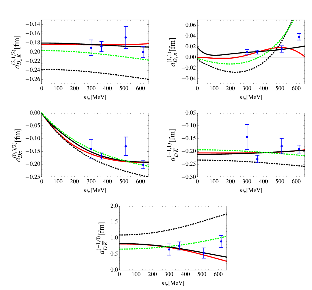
Fitting these unknown LECs to the lightest 15 LQCD data, we obtain the results shown in Fig. 1, with the corresponding LECs tabulated in Table I. At leading order, the $\chi^{2}/\mathrm{d.o.f}\approx 17.9$ is rather poor, indicating the failure of a quantitative description of the LQCD data.⁴⁴ 4 The same is true for the on-shell approach. On the other hand, if one would use the SU(3) average of the pseudoscalar decay constants, $f_{0}=1.15f_{\pi}$ , instead of $f_{\pi}$ , the $\chi^{2}/\mathrm{d.o.f}$ would be reduced to about $3.9$ . At next-to-leading order, we obtain a $\chi^{2}/\mathrm{d.o.f}\approx 0.79$ , which should be compared to that obtained in the on-shell approximation, $\chi^{2}/\mathrm{d.o.f}=1.23$ [26].⁵⁵ 5 It should be mentioned that one could still obtain a $\chi^{2}/\mathrm{d.o.f.}\approx 0.89$ by fitting the whole 20 LQCD data points in the off-shell approach. Furthermore, it is interesting to note that the off-shell results and the on-shell results differ most for $a_{D_{s}\pi}$ in the $(S=1,I=1)$ channel, which couples $D_{s}\pi$ to $DK$ [23].

Clearly, the off-shell effects seem to improve the description of the LQCD data of Ref. [23]. This result should not be a total surprise. In Refs.[3, 4], it was pointed out that the off-shell effects, which manifest themselves through diagrams renormalizing the vertices and the hadron masses, can be absorbed by the available LECs and physical masses. Of course, such ‘‘renormalizations’’ are only possible at the physical point, because otherwise one may have to use light-quark mass dependent couplings.⁶⁶ 6 The hadron masses have to be light-quark mass dependent anyway. Therefore, to study the light-quark mass evolution of physical observables, one may wish to explicitly keep all the off-shell effects. Our results show that this may indeed improve the description of light-quark mass dependence. Nevertheless, more studies are needed in order to confirm that this is generally true.

The LQCD simulations of Ref. [23] did not include the ( $S=1,I=0)$ channel where the $D^{*}_{s0}(2317)$ appears. The studies in Refs. [23, 26] show that a fit to the LQCD data yields naturally the $D^{*}_{s0}(2317)$ in UChPT. It will be interesting to check whether this still holds in the present formalism. Searching for a pole in the complex plane, we find a bound state at $\sqrt{s}=2.295$ GeV, which is not so far away from the $D^{*}_{s0}(2317)$ pole position from the on-shell approach, $\sqrt{s}=2.317$ GeV, which coincides with the experimental measurement. The discrepancy of about 22 MeV provides another indicator on the magnitude of the off-shell effects.

In Fig. 2, we show the pion mass and kaon mass evolution of the $D^{*}_{s0}(2317)$ . To facilitate the comparison, we have shifted the off-shell results by $22$ MeV so that the on-shell and off-shell results agree at the physical point. The figure in the left panel is obtained by fixing the strange quark mass to its physical value using the leading-order ChPT, while the figure in the right panel is obtained by fixing the pion mass to its physical value. The dependences of the $D$ and $D_{s}$ masses on the pion and kaon masses are provided by the next-to-leading-order ChPT as in Ref. [26]. It is clear that for the light-quark mass evolution of the $D^{*}_{s0}(2317)$ pole position there is no appreciable difference between the on-shell and off-shell UChPT.

IV Summary

We have solved the Bethe-Salpeter equation in unitarized chiral perturbation theory by taking into account the off-shell terms of the chiral potentials up to next-to-leading order. To quantify the magnitude and impact of the off-shell effects, we have studied the latest $n_{f}=2+1$ LQCD simulations of the scattering lengths of Nambu-Goldstone bosons off $D$ mesons. In comparison with the widely used on-shell approximation, we have shown that taking into account off-shell effects can indeed improve the description of the LQCD data, in terms of light-quark mass evolution. On the other hand, both descriptions look qualitatively similar, at least for the observables we studied. Therefore, unless the LQCD data become more precise, the on-shell approximation may still be confidently used, given its simplicity.

V Acknowledgements

M. A. and L. S. G. thank Norbert Kaiser and Wolfram Weise for enlightening discussions and a careful reading of the manuscript. This work is supported in part by BMBF, by the A.v. Humboldt foundation, the Fundamental Research Funds for the Central Universities, the National Natural Science Foundation of China (Grant No. 11005007), the New Century Excellent Talents in University Program of Ministry of Education of China under Grant No. NCET-10-0029, the DFG Cluster of Excellence “Origin and Structure of the Universe,” and by DFG and NSFC through the Sino-German CRC 110 “Symmetries and Emergence of Structure in QCD.”

VI Appendix

In this appendix we present more details on how the Bethe-Salpeter equation with full off-shell potentials is solved. For the sake of simplicity, we restrict ourselves to the case with the kernel being the leading-order Weinberg-Tomozawa term. In this case, one only needs to introduce a three-component vector $B$ ,

B(q,P,M,\mu)^{T}=\left(\frac{q^{2}-M^{2}}{f_{0}^{2}},\frac{P_{\mu}+q_{\mu}}{f_{0}},1\right)\,,

(17)

instead of a four-component vector as done in the main text. The Weinberg-Tomazawa potential can then be represented in the following way:

$\displaystyle V_{\mathrm{WT}}(q,Q,P)$	$\displaystyle=$	$\displaystyle\frac{\mathcal{C}_{\mathrm{LO}}}{4f_{0}^{2}}(2P^{2}-2(P+q)\cdot(P+Q)-q^{2}-Q^{2})$	(18)
	$\displaystyle=$	$\displaystyle B(q,P,M_{1},\nu)^{T}\cdot\hat{V}_{\mathrm{WT}}(\nu,\mu)\cdot B(Q,P,M_{3},\mu)$
	$\displaystyle\equiv$	$\displaystyle B(q)^{T}\cdot\hat{V}_{\mathrm{WT}}\cdot B(Q)\,,$

where

\hat{V}_{\mathrm{WT}}(\nu,\mu)=\mathcal{C}_{\textrm{LO}}\left(\begin{array}[]{cccc}0&0&-\frac{1}{4}\\ 0&-\frac{g^{\mu\nu}}{2}&0\\ -\frac{1}{4}&0&\frac{1}{4f_{0}^{2}}\left(2P^{2}-M_{1}^{2}-M_{3}^{2}\right)\end{array}\right)\,.

(19)

In the last line of Eq. (18) we have introduced a brief notation such that the summation over Lorentz indices and the dependence on $P$ , $M_{1}$ , and $M_{3}$ are implicit. The idea behind this matrix representation of the potential is that the dependence on the loop momenta, here $q$ and $Q$ , can be absorbed into the vector $B$ or the loop matrix $\hat{G}$ as defined in Eq. (9). In the present case, the loop matrix becomes a $3\times 3$ matrix (instead of $4\times 4$ ),

\displaystyle\hat{G}(\nu,\mu)

\displaystyle\equiv

\displaystyle\left(\begin{array}[]{ccc}G_{11}(s)&0&G_{13}(s)\\ 0&g^{\mu\nu}G_{22a}(s)+P^{\mu}P^{\nu}G_{22b}(s)&P^{\nu}G_{23}(s)\\ G_{13}(s)&P^{\mu}G_{23}(s)&G_{33}(s)\end{array}\right)\,.

With these definitions, the leading one-loop diagram of the infinite sum illustrated in Fig. 3 simply reads

			$\displaystyle B(q,P,M_{1},\nu)^{T}\cdot\hat{V}_{\mathrm{WT}}(\nu,\rho)\cdot\hat{G}(\rho,\sigma)\cdot\hat{V}_{\mathrm{WT}}(\sigma,\mu)\cdot B(Q,P,M_{3},\mu)$		(24)
		$\displaystyle\equiv$	$\displaystyle B(q)^{T}\cdot\hat{V}_{\mathrm{WT}}\cdot\hat{G}\cdot\hat{V}_{\mathrm{WT}}\cdot B(Q)\,,$		(24)

and the Bethe-Salpeter equation becomes

	$\displaystyle B(q)^{T}\cdot\hat{T}\cdot B(Q)$	$\displaystyle=$	$\displaystyle B(q)^{T}\cdot(\hat{V}_{\mathrm{WT}}+\hat{V}_{\mathrm{WT}}\cdot\hat{G}\cdot\hat{V}_{\mathrm{WT}}+\hat{V}_{\mathrm{WT}}\cdot\hat{G}\cdot\hat{V}_{\mathrm{WT}}\cdot\hat{G}\cdot\hat{V}_{\mathrm{WT}}+\ldots)\cdot B(Q)$		(25)
		$\displaystyle=$	$\displaystyle B(q)^{T}\cdot(\hat{V}_{\mathrm{WT}}+\hat{V}_{\mathrm{WT}}\cdot\hat{G}\cdot\hat{T})\cdot B(Q)\,.$		(25)

It is clear that $\hat{T}$ still corresponds to a geometric series, as in the on-shell approximation case. One can easily deduce that $\hat{T}$ is of the following form

\displaystyle\hat{T}(\nu,\mu)\equiv\left(\footnotesize{\begin{array}[]{cccc}t_{11}&P^{\mu}t_{12}&t_{13}\\ P^{\nu}t_{21}&g^{\mu\nu}t_{22a}+P^{\mu}P^{\nu}t_{22b}&P^{\nu}t_{23}\\ t_{31}&P^{\mu}t_{32}&t_{33}\end{array}}\right)\,,

where the functions $t_{i}$ depend on the involved masses and the total four-momentum squared $s=P^{2}$ . One should notice that Lorentz indices in $\hat{T}$ can only be carried by the metric tensor $g^{\mu\nu}$ or the total momentum $P^{\mu}$ ( $P^{\nu}$ ). More explicitly, for a single-channel process ( $M_{1}=M_{3}=M$ ), the Bethe-Salpeter equation

\hat{T}=\hat{V}_{\mathrm{WT}}+\hat{V}_{\mathrm{WT}}\cdot\hat{G}\cdot\hat{T}

(30)

gives a set of coupled linear equations,

\displaystyle\begin{array}[]{lll}t_{11}&=&-\frac{1}{4}\mathcal{C}_{\mathrm{LO}}\left(G_{23}P^{2}t_{21}+G_{13}t_{11}+G_{33}t_{31}\right)\\ t_{12}&=&-\frac{1}{4}\mathcal{C}_{\mathrm{LO}}\left(G_{23}\left(t_{22a}+P^{2}t_{22b}\right)+G_{13}t_{12}+G_{33}t_{32}\right)\\ t_{13}&=&-\frac{1}{4}\mathcal{C}_{\mathrm{LO}}\left(G_{23}P^{2}t_{23}+G_{13}t_{13}+G_{33}t_{33}+1\right)\\ t_{21}&=&-\frac{1}{2}\mathcal{C}_{\mathrm{LO}}\left(t_{21}G_{22a}+P^{2}t_{21}G_{22b}+G_{23}t_{31}\right)\\ t_{22a}&=&-\frac{1}{2}\mathcal{C}_{\mathrm{LO}}\left(G_{22a}t_{22a}+1\right)\\ t_{22b}&=&-\frac{1}{2}\mathcal{C}_{\mathrm{LO}}\left(G_{22b}\left(t_{22a}+P^{2}t_{22b}\right)+G_{22a}t_{22b}+G_{23}t_{32}\right)\\ t_{23}&=&-\frac{1}{2}\mathcal{C}_{\mathrm{LO}}\left(t_{23}G_{22a}+P^{2}t_{23}G_{22b}+G_{23}t_{33}\right)\\ t_{31}&=&-\frac{1}{4}\mathcal{C}_{\mathrm{LO}}\left(-2\Delta G_{23}P^{2}t_{21}-2\Delta G_{33}t_{31}+G_{13}\left(t_{31}-2\Delta t_{11}\right)+G_{11}t_{11}+1\right)\\ t_{32}&=&-\frac{1}{4}\mathcal{C}_{\mathrm{LO}}\left(-2\Delta\left(G_{23}\left(t_{22a}+P^{2}t_{22b}\right)+G_{33}t_{32}\right)+G_{13}\left(t_{32}-2\Delta t_{12}\right)+G_{11}t_{12}\right)\\ t_{33}&=&\frac{1}{4}\mathcal{C}_{\mathrm{LO}}\left(2\Delta\left(G_{23}P^{2}t_{23}+G_{33}t_{33}+1\right)+G_{13}\left(2\Delta t_{13}-t_{33}\right)-G_{11}t_{13}\right)\,,\end{array}

with $\Delta=(P^{2}-M^{2})/f_{0}^{2}$ . These equations determine all the $t_{i}$ ’s introduced in Eq. (VI). The generalization to coupled channels is straightforward.

References

[1] N. Kaiser, P. B. Siegel and W. Weise, Nucl. Phys. A 594, 325 (1995) [nucl-th/9505043].
[2] A. Dobado and J. R. Pelaez, Phys. Rev. D 56, 3057 (1997) [hep-ph/9604416].
[3] J. A. Oller and E. Oset, Nucl. Phys. A 620, 438 (1997) [Erratum-ibid. A 652, 407 (1999)] [hep-ph/9702314].
[4] E. Oset and A. Ramos, Nucl. Phys. A 635, 99 (1998) [nucl-th/9711022].
[5] J. A. Oller, E. Oset and J. R. Pelaez, Phys. Rev. D 59, 074001 (1999) [Erratum-ibid. D 60, 099906 (1999)] [Erratum-ibid. D 75, 099903 (2007)] [hep-ph/9804209].
[6] N. Kaiser, Eur. Phys. J. A 3, 307 (1998).
[7] J. A. Oller and E. Oset, Phys. Rev. D 60, 074023 (1999) [hep-ph/9809337].
[8] J. A. Oller and U. G. Meissner, Phys. Lett. B 500, 263 (2001) [hep-ph/0011146].
[9] M. F. M. Lutz and E. E. Kolomeitsev, Nucl. Phys. A 700, 193 (2002) [nucl-th/0105042].
[10] A. Martinez Torres, K. P. Khemchandani, L. S. Geng, M. Napsuciale and E. Oset, Phys. Rev. D 78, 074031 (2008) [arXiv:0801.3635 [nucl-th]].
[11] P. Wang and X. G. Wang, Phys. Rev. Lett. 111, 042002 (2013) arXiv:1304.0846 [hep-ph].
[12] E. E. Salpeter and H. A. Bethe, Phys. Rev. 84, 1232 (1951).
[13] J. Nieves and E. Ruiz Arriola, Phys. Lett. B 455, 30 (1999) [nucl-th/9807035].
[14] J. Nieves and E. Ruiz Arriola, Nucl. Phys. A 679, 57 (2000) [hep-ph/9907469].
[15] J. Nieves and E. Ruiz Arriola, Phys. Rev. D 63, 076001 (2001) [hep-ph/0008034].
[16] J. Nieves and E. Ruiz Arriola, Phys. Rev. D 64, 116008 (2001) [hep-ph/0104307].
[17] D. Djukanovic, J. Gegelia and S. Scherer, Eur. Phys. J. A 29, 337 (2006) [hep-ph/0604164].
[18] B. Borasoy, P. C. Bruns, U. -G. Meissner and R. Nissler, Eur. Phys. J. A 34, 161 (2007) [arXiv:0709.3181 [nucl-th]].
[19] P. C. Bruns, M. Mai and U. G. Meissner, Phys. Lett. B 697, 254 (2011) [arXiv:1012.2233 [nucl-th]].
[20] M. Mai, P. C. Bruns and U. -G. Meissner, Phys. Rev. D 86, 094033 (2012) [arXiv:1207.4923 [nucl-th]].
[21] C. Hanhart, J. R. Pelaez and G. Rios, Phys. Rev. Lett. 100, 152001 (2008) [arXiv:0801.2871 [hep-ph]].
[22] M. Cleven, F. -K. Guo, C. Hanhart and U. -G. Meissner, Eur. Phys. J. A 47, 19 (2011) [arXiv:1009.3804 [hep-ph]].
[23] L. Liu, K. Orginos, F. -K. Guo, C. Hanhart and U. -G. Meissner, Phys. Rev. D 87, 014508 (2013) [arXiv:1208.4535 [hep-lat]].
[24] F. -K. Guo, C. Hanhart and U. -G. Meissner, Eur. Phys. J. A 40, 171 (2009) [arXiv:0901.1597 [hep-ph]].
[25] P. Wang and X. G. Wang, Phys. Rev. D 86, 014030 (2012) [arXiv:1204.5553 [hep-ph]].
[26] M. Altenbuchinger, L. -S. Geng and W. Weise, Phys. Rev. D 89, 014026 (2014) [arXiv:1309.4743 [hep-ph]].
[27] G. ’t Hooft and M. J. G. Veltman, Nucl. Phys. B 153, 365 (1979).
[28] E. E. Jenkins and A. V. Manohar, Phys. Lett. B 255, 558 (1991).
[29] T. Becher and H. Leutwyler, Eur. Phys. J. C 9, 643 (1999) [hep-ph/9901384].
[30] T. Fuchs, J. Gegelia, G. Japaridze and S. Scherer, Phys. Rev. D 68, 056005 (2003) [hep-ph/0302117].
[31] L. S. Geng, Front. Phys. China. 8, 328 (2013) [arXiv:1301.6815 [nucl-th]].
[32] D. Mohler, S. Prelovsek and R. M. Woloshyn, Phys. Rev. D 87, 034501 (2013) [arXiv:1208.4059 [hep-lat]].
[33] D. Mohler, C. B. Lang, L. Leskovec, S. Prelovsek and R. M. Woloshyn, Phys. Rev. Lett. 111, 222001 (2013) [arXiv:1308.3175 [hep-lat]].
[34] J. Beringer et al. [Particle Data Group Collaboration], Phys. Rev. D 86, 010001 (2012).

Off-shell effects on the interaction of Nambu-Goldstone bosons and DD mesons