Discriminative Measures for Comparison of Phylogenetic Trees

Omur Arslan Email: omur@seas.upenn.edu Dan P. Guralnik Email: guralnik@seas.upenn.edu Daniel E. Koditschek Email: kod@seas.upenn.edu Address: Department of Electrical and Systems Engineering, University of Pennsylvania, Philadelphia, PA 19104, USA

Abstract

In this paper we introduce and study three new measures for efficient discriminative comparison of phylogenetic trees. The NNI navigation dissimilarity $\mathit{d}_{nav}$ counts the steps along a “combing” of the Nearest Neighbor Interchange (NNI) graph of binary hierarchies, providing an efficient approximation to the (NP-hard) NNI distance in terms of “edit length”. At the same time, a closed form formula for $\mathit{d}_{nav}$ presents it as a weighted count of pairwise incompatibilities between clusters, lending it the character of an edge dissimilarity measure as well. A relaxation of this formula to a simple count yields another measure on all trees — the crossing dissimilarity $\mathit{d}_{CM}$ . Both dissimilarities are symmetric and positive definite (vanish only between identical trees) on binary hierarchies but they fail to satisfy the triangle inequality. Nevertheless, both are bounded below by the widely used Robinson-Foulds metric and bounded above by a closely related true metric, the cluster-cardinality metric $\mathit{d}_{CC}$ . We show that each of the three proposed new dissimilarities is computable in time $\mathrm{O}(n^{2})$ in the number of leaves $n$ , and conclude the paper with a brief numerical exploration of the distribution over tree space of these dissimilarities in comparison with the Robinson-Foulds metric and the more recently introduced matching-split distance.

Keywords:

Phylogenetic Trees, Evolutionary Trees, Nearest Neighbor Interchange, Comparison of Classifications, Tree Metric.

\nopreprintlinetrue

1 Introduction

1.1 Motivation

A fundamental classification problem common to both computational biology and engineering is the efficient and informative comparison of hierarchical structures. In bioinformatics settings, these typically take the form of phylogenetic trees representing evolutionary relationships within a set $S$ of taxa. In pattern recognition and data mining settings, hierarchical trees are often used to encode nested sequences of groupings of a set of observations. Dissimilarity between combinatorial trees has been measured in the past literature largely by recourse to one of two separate approaches: comparing edges and counting edit distances. Representing the former approach, a widely used tree metric is the Robinson-Foulds (RF) distance, $\mathit{d}_{RF}$ , [1] whose count of the disparate edges between trees requires linear time, $\mathrm{O}(n)$ , in the number of leaves, $n$ , to compute [2]. Empirically, $\mathit{d}_{RF}$ offers only a very coarse measure of disparity, and among its many proposed refinements, the recent matching split distance $\mathit{d}_{MS}$ , [3, 4] offers a more discriminative metric albeit with considerably higher computational cost, $\mathrm{O}(n^{2.5}\log n)$ . Alternatively, various edit distances have been proposed [5, 6, 7, 8] but the most natural variant, the Nearest Neighbor Interchange (NNI) distance $\mathit{d}_{NNI}$ , entails an NP-complete computation for both labelled and unlabelled trees [9].

1.2 Results

Our main contribution is the introduction of a dissimilarity measure on the space $\mathcal{BT}_{S}$ of labelled binary trees which bridges the above approaches by what is, effectively, a solution to the NNI navigation problem in $\mathcal{BT}_{S}$ :

Problem 1 (NNI Navigation Problem).

Given a target $\tau\in\mathcal{BT}_{S}$ , provide an efficient algorithm $\mathcal{A}_{\tau}$ which, for any $\sigma\in\mathcal{BT}_{S}$ , computes a Nearest Neighbor Interchange to be performed on $\sigma$ while guaranteeing that successive application of $\mathcal{A}_{\tau}$ terminates in $\tau$ .

This problem is motivated by applications in coordinated robot navigation [10, 11, 12], where a group of robots is required to reconfigure reactively in real time their (structural) adjacencies while navigating towards a desired goal configuration. Thus, our particular formulation of the problem is inspired by the notion of reactive planning [13], but may likely hold value for researchers interested in tree consensus and averaging as well.

Of course, since computation of $\mathit{d}_{NNI}$ is NP-hard, one cannot hope for repeated applications of $\mathcal{A}_{\tau}$ to produce NNI geodesics without incurring prohibitive complexity in each iteration. However, as we will show, constructing an efficient navigation scheme is possible if we allow the algorithm to produce less restricted paths: for $\left|S\right|=n$ , our navigation algorithms require $\mathrm{O}(n)$ time for each iteration and produce paths of length $\mathrm{O}(n^{2})$ (as compared to the $\mathrm{O}(n\log n)$ diameter of $\mathit{d}_{NNI}$ — see (19)).

Additional insight into the geometry of the space $(\mathcal{BT}_{S},\mathit{d}_{NNI})$ is gained by recognizing a significant degree of freedom with which our navigation algorithm may select the required tree restructuring operation at each stage. As it turns out, for any given target $\tau$ , the repeated application of $\mathcal{A}_{\tau}$ to a tree $\sigma$ until reaching $\tau$ will yield paths of equal lengths regardless of any choices made along the way. This length, by definition, is the navigation dissimilarity $\mathit{d}_{nav}\left(\sigma,\tau\right)$ (and is obtained, in the manner described, in $\mathrm{O}(n^{3})$ time, though more efficient implementations will guarantee $\mathrm{O}(n^{2})$ ). At the same time, a closed form formula we derive for $\mathit{d}_{nav}$ allows us to avoid computing a navigation path when only the value of $\mathit{d}_{nav}$ is needed, and computes it in $\mathrm{O}(n^{2})$ time. Surprisingly, despite the asymmetric character of its construction, $\mathit{d}_{nav}$ is a symmetric (and positive definite) dissimilarity on $\mathcal{BT}_{S}$ , though it fails to be a metric.

Although $\mathit{d}_{nav}$ does not satisfy the triangle inequality, it is related to the well accepted Robinson-Foulds distance by the following tight bounds:

\mathit{d}_{RF}\leq\mathit{d}_{nav}\leq\frac{1}{2}\mathit{d}_{RF}^{2}+\frac{1}{2}\mathit{d}_{RF}~,

(1)

We find it useful to introduce a “relaxation” of $\mathit{d}_{nav}$ , the crossing dissimilarity $\mathit{d}_{CM}$ . This dissimilarity simply counts all the pairwise cluster incompatibilities between two trees, hence it is symmetric, positive-definite, and computable in $\mathrm{O}(n^{2})$ time. In fact, the two dissimilarities are commensurable, leading to similar bounds in terms of $\mathit{d}_{RF}$ :

\mathit{d}_{CM}\leq\mathit{d}_{nav}\leq\frac{3}{2}\mathit{d}_{CM}\,,\quad\mathit{d}_{RF}\leq\mathit{d}_{CM}\leq\mathit{d}_{RF}^{2}~.

(2)

Finally, we introduce a true metric whose spatial resolution and computational complexity is comparable to those our new dissimilarities. Exploiting a well known relation between trees and ultrametrics [14], we also introduce the cluster-cardinality distance $\mathit{d}_{CC}$ — constructed as the pullback of a matrix norm along an embedding of hierarchies into the space of matrices and computable in $\mathrm{O}(n^{2})$ time — which is a true metric bounding $\mathit{d}_{CM}$ from above (and hence also $\mathit{d}_{nav}$ , up to a constant factor). Thus, cumulatively we obtain:

\frac{2}{3}\mathit{d}_{RF}\leq\frac{2}{3}\mathit{d}_{nav}\leq\mathit{d}_{CM}\leq\mathit{d}_{CC}~.

(3)

We have surveyed some of the new features of our tree proximity measures that might hold interest for pattern classification and phylogeny analysis relative to the diverse alternatives that have appeared in the literature. Closest among these many alternatives [15, 16, 17], $\mathit{d}_{nav}$ has some resemblance to an early NNI graph navigation algorithm, $\mathit{d}_{ra}$ [17] which used a divide-and-conquer approach with a balancing strategy to achieve an $\mathrm{O}(n\log n)$ computation of tree dissimilarity. Notwithstanding its lower computational cost, in contrast to $\mathit{d}_{nav}$ , the recursive definition of $\mathit{d}_{ra}$ , as with many NNI distance approximations [15, 16, 17], does not admit a closed form expression.

It is often of interest to compare more than pairs of hierarchies at a time, and the notion of a “consensus” tree has accordingly claimed a good deal of attention in the literature [18]. For instance, the majority rule tree [19] of a set of trees is a median tree respecting the RF distance and provides statistics on the central tendency of trees [20]. When $\mathit{d}_{nav}$ and $\mathit{d}_{CM}$ are extended to degenerate trees they fail to be positive definite, and thus their behavior over (typically degenerate) consensus trees departs still further from the properties of a true metric. However, it turns out that both notions of a consensus tree (strict [21], and loose/semi-strict [22]) behave as median trees with respect to both our dissimilarities. In fact, the loose consensus tree is the maximal (finest) median tree with respect to inclusion for both $\mathit{d}_{nav}$ and $\mathit{d}_{CM}$ .

The paper is organized as follows. Section 2 briefly summarizes the necessary background while introducing the notation used throughout the sequel. Section 3 introduces and studies the cluster-cardinality distance $\mathit{d}_{CC}$ and the crossing dissimilarity $\mathit{d}_{CM}$ . In Section 4 we present a solution of the NNI navigation problem and study properties of the resulting NNI navigation dissimilarity $\mathit{d}_{nav}$ and its relations with other tree dissimilarity measures. Section 5 discusses the relation between commonly used consensus models and our tree dissimilarities $\mathit{d}_{CM}$ and $\mathit{d}_{nav}$ , and compares our proposed tree measures with $\mathit{d}_{RF}$ and $\mathit{d}_{MS}$ based on some frequently used empirical distributions of tree measures. A brief discussion of future directions follows in Section 6.

2 Preliminaries

2.1 Hierarchies

By a hierarchy $\tau$ over a fixed non-empty finite index set $S$ we shall mean a rooted tree with labeled leaves (see Figure 1). Formally, $\tau$ is a finite connected acyclic graph with leaves (vertices of degree one) bijectively labelled by $S$ , and edges oriented in such a way that (i) all interior vertices have out-degree at least two, and (ii) there is a vertex, referred to as the root of $\tau$ , such that every edge is oriented away from the root. Under these assumptions all the vertices of $\tau$ are reachable from the root through a directed path in $\tau$ [23].

The cluster $\mathcal{C}\left(v\right)$ of a vertex $v\in V_{\tau}$ of a hierarchy $\tau$ is defined to be the set of leaves reachable from $v$ by a directed path in $\tau$ . Singleton clusters and the root cluster $S$ are common to all trees, and we refer to them as the trivial clusters. We denote by $\mathcal{C}\left(\tau\right)$ (respectively $\mathcal{C}_{int}\left(\tau\right)$ ) the set of all clusters (resp. non-trivial clusters) of $\tau$ :

\mathcal{C}\left(\tau\right)\>{\mathbf{:}=}\>\left\{\mathcal{C}\left(v\right)\big|\,v\in V_{\tau}\right\}\subseteq\mathcal{P}\left(S\right)~,\qquad\mathcal{C}_{int}\left(\tau\right)\>{\mathbf{:}=}\>\left\{I\in\mathcal{C}\left(\tau\right)\setminus\left\{S\right\}\Big|\left|I\right|\geq 2\right\}~,

(4)

where $\mathcal{P}\left(S\right)$ denotes the power set of $S$ .

2.1.1 Compatibility

Definition 1 ([24, 8]).

Subsets $A,B\subset S$ are said to be compatible, $A\bowtie B$ , if

A\cap B=\varnothing\;\vee\;A\subseteq B\;\vee\;B\subseteq A~.

(5)

If $A\not\bowtie B$ , then we say that $A$ and $B$ cross. We further extend the compatibility relation $(\bowtie)$ as follows:

•

For $\mathcal{A},\mathcal{B}\subseteq\mathcal{P}\left(S\right)$ , write $\mathcal{A}\bowtie\mathcal{B}~$ if $~A\bowtie B$ for all $A\in\mathcal{A}$ and $B\in\mathcal{B}$ ;
•

For a cluster $I\subseteq S$ and a tree $\tau$ over the leaf set $S$ , write $I\bowtie\tau~$ if $~\left\{I\right\}\bowtie\mathcal{C}\left(\tau\right)$ ;
•

For two trees $\sigma$ and $\tau$ over the leaf set $S$ , write $\sigma\bowtie\tau~$ if $~\mathcal{C}\left(\sigma\right)\bowtie\mathcal{C}\left(\tau\right)$ .

By construction, any two elements of $\mathcal{C}\left(\tau\right)$ are compatible for any tree $\tau$ . This motivates the following definition:

Definition 2 ([24]).

A subset $\mathcal{A}$ of $\mathcal{P}\left(S\right)$ is said to be nested — also referred to in the literature as a “laminar family” — if any two elements of $\mathcal{A}$ are compatible. $\mathcal{C}\left(\tau\right)$ is known as the laminar family associated with $\tau$ .

2.1.2 Hierarchical Relations

Refer to caption — Figure 1: Hierarchical Relations: ancestors - $\mathrm{Anc}\left(I,\tau\right)$ , parent - $\mathrm{Pr}\left(I,\tau\right)$ , children - $\mathrm{Ch}\left(I,\tau\right)$ , descendants - $\mathrm{Des}\left(I,\tau\right)$ , and local complement (sibling) - ${I}^{-\tau}$ of cluster $I$ of a rooted binary phylogenetic tree, $\tau\in\mathcal{BT}_{\left[13\right]}$ . Filled and unfilled circles represent interior and leaf nodes, respectively. An interior node is referred to by its cluster, the list of leaves below it; for example, $I=\left\{4,5,6,7\right\}$ . Accordingly, the cluster set of $\tau$ is $\mathcal{C}\left(\tau\right)=\left\{\big.\right.\!\!\left\{1\right\},\left\{2\right\},\ldots,\left\{13\right\},\left\{1,2\right\},\left\{1,2,3\right\},\left\{4,5\right\},\left\{6,7\right\},\left\{4,5,6,7\right\},\left\{1,2,\ldots,7\right\},\left\{9,10\right\},\left\{8,9,10\right\},\left\{11,12\right\},\left\{11,12,13\right\},\left\{8,9,\ldots,13\right\},\left\{1,2,\ldots,13\right\}\!\!\left.\big.\right\}$ .

The cluster set $\mathcal{C}\left(\tau\right)$ of a hierarchy $\tau$ completely determines its representation as a rooted tree with labeled leaves: $\mathcal{C}\left(\tau\right)$ stands in bijective correspondence with the vertex set of $\tau$ , and $(v,v^{\prime})$ is an edge in $\tau$ if and only if $\mathcal{C}\left(v\right)\supset\mathcal{C}\left(v^{\prime}\right)$ and there is no $\tilde{v}\in V_{\tau}$ such that $\mathcal{C}\left(v\right)\supset\mathcal{C}\left(\tilde{v}\right)\supset\mathcal{C}\left(v^{\prime}\right)$ . Consequently, the standard notions of ancestor, descendant, parent and child of a vertex in common use for rooted trees carry over to the cluster representation as follows:


$\displaystyle\mathrm{Anc}\left(I,\tau\right)$	$\displaystyle=\left\{V\hskip-1.42262pt\in\hskip-1.42262pt\mathcal{C}\left(\tau\right)\big\|\,I\subsetneq V\right\},$	$\displaystyle\mathrm{Des}\left(I,\tau\right)$	$\displaystyle=\left\{V\hskip-1.42262pt\in\hskip-1.42262pt\mathcal{C}\left(\tau\right)\big\|\,V\subsetneq I\right\},$	(6a)
$\displaystyle\mathrm{Pr}\left(I,\tau\right)$	$\displaystyle=\min\left(\mathrm{Anc}\left(I,\tau\right)\right),$	$\displaystyle\mathrm{Ch}\left(I,\tau\right)$	$\displaystyle=\left\{V\in\mathcal{C}\left(\tau\right)\big\|\,\mathrm{Pr}\left(V,\tau\right)=I\right\},$	(6b)

where $\min\left(\mathrm{Anc}\left(I,\tau\right)\right)$ is computed with respect to the inclusion order. Note that for the trivial clusters we have $\mathrm{Pr}\left(S,\tau\right)=\varnothing$ and $\mathrm{Ch}\left(\{s\},\tau\right)=\varnothing$ for $s\in S$ .

Since the set of children partitions each parent, we find it useful to define the local complement ${I}^{-\tau}$ of $I\in\mathcal{C}\left(\tau\right)$ as

{I}^{-\tau}\>{\mathbf{:}=}\>\mathrm{Pr}\left(I,\tau\right)\setminus I~,

(7)

not to be confused with the standard (global) complement, ${I}^{C}=S\setminus I$ . Further, a grandchild in $\tau$ is a cluster $G\in\mathcal{C}\left(\tau\right)$ having a grandparent $\mathrm{Pr}^{2}\left(G,\tau\right)\>{\mathbf{:}=}\>\mathrm{Pr}\left(\big.\mathrm{Pr}\left(G,\tau\right),\tau\right)$ in $\tau$ . We denote the set of all grandchildren in $\tau$ by $\mathcal{G}\left(\tau\right)$ ,

\mathcal{G}\left(\tau\right)\>{\mathbf{:}=}\>\left\{G\in\mathcal{C}\left(\tau\right)\big|\,\mathrm{Pr}^{2}\left(G,\tau\right)\neq\varnothing\right\}~.

(8)

If $A,B$ are either elements of $S$ or clusters of $\tau$ , it is convenient to have $\left(A{\wedge}B\right)_{\tau}$ denote the smallest (in terms of cardinality) common ancestor of $A$ and $B$ in $\tau$ . Finally, the depth $0pt{\tau}(I)$ of a cluster in a hierarchy $\tau$ is defined to equal the number of distinct ancestors of $I$ in $\tau$ .

2.1.3 Nondegeneracy

A rooted tree where every interior vertex has exactly two children is said to be binary or non-degenerate. All other trees are said to be degenerate. We will denote the set of hierarchies over a finite leaf set $S$ , by $\mathcal{T}_{S}$ . The subset of non-degenerate hierarchies will be denoted by $\mathcal{BT}_{S}$ .

Note that the laminar family $\mathcal{C}\left(\tau\right)$ of a degenerate tree $\tau$ may always be augmented with additional clusters while remaining nested (Definition 2). This leads to the well known result:

Remark 1 ([25, 24]).

Let $\tau\in\mathcal{T}_{S}$ . Then $\tau$ has at most $2\left|S\right|-1$ vertices, with equality if and only if $\tau$ is nondegenerate, if and only if $\mathcal{C}\left(\tau\right)$ is a maximal laminar family in $\mathcal{P}\left(S\right)$ with respect to inclusion.¹¹ 1 In this paper we adopt the convention that a laminar family does not contain the empty set (as an element).

2.1.4 Consensus

Definition 3 ([21, 22]).

For any set of trees $T$ in $\mathcal{T}_{S}$ , the strict and loose consensus trees of $T$ , denoted $T_{\ast}$ and $T^{\ast}$ respectively, are defined by specifying their cluster sets as follows:

\mathcal{C}\left(T_{\ast}\right)=\bigcap_{\tau\in T}\mathcal{C}\left(\tau\right)\,,\quad\mathcal{C}\left(T^{\ast}\right)=\left\{I\in\bigcup_{\tau\in T}\mathcal{C}\left(\tau\right)\Bigg|\,\forall\sigma\in T\quad I\bowtie\sigma\right\}.

(9)

Note that the loose consensus tree $T^{\ast}$ of $T$ refines the strict consensus tree $T_{\ast}$ , that is $\mathcal{C}\left(T^{\ast}\right)\supseteq\mathcal{C}\left(T_{\ast}\right)$ .

2.2 Some Operations on Trees

2.2.1 The NNI Graph

The standard definition of NNI walks on unrooted binary trees [5, 6] conveniently restricts to the space $\mathcal{BT}_{S}$ of rooted binary trees as follows:

Definition 4.

Let $\sigma\in\mathcal{BT}_{S}$ . We say that $\tau\in\mathcal{BT}_{S}$ is the result of performing a Nearest Neighbor Interchange (NNI) move on $\sigma$ at a grandchild $G\in\mathcal{G}\left(\sigma\right)$ (8) if

\mathcal{C}\left(\tau\right)=\left(\Big.\mathcal{C}\left(\sigma\right)\setminus\left\{\big.\mathrm{Pr}\left(G,\sigma\right)\right\}\right)\cup\left\{\big.\mathrm{Pr}^{2}\left(G,\sigma\right)\setminus G\right\}.

(10)

We often indicate this by writing $\tau=\text{NNI}(\sigma,G)$ .

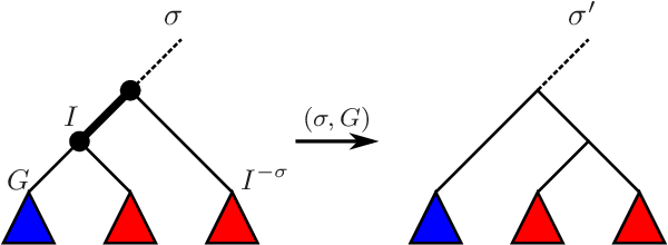
Note that the NNI move at cluster $G$ on $\sigma$ swaps cluster $G$ with its parent’s sibling ${\mathrm{Pr}\left(G,\sigma\right)}^{-\sigma}$ to yield $\tau$ , depicted in Figure 2(left); and after an NNI move at cluster $G$ of $\sigma$ , grandchild $G$ of grandparent $P=\mathrm{Pr}^{2}\left(G,\sigma\right)$ with respect to $\sigma$ becomes child $G$ of parent $P=\mathrm{Pr}\left(G,\tau\right)$ with respect to $\tau$ .

It is standard to say that $\sigma,\tau\in\mathcal{BT}_{S}$ are NNI-adjacent if and only if one can be obtained from the other by a single move. Figure 2(left) illustrates the moves on $\mathcal{BT}_{S}$ and their inverses.

The NNI-graph is formed over the vertex set $\mathcal{BT}_{S}$ by declaring two trees to be connected by an edge if and only if they are NNI-adjacent, see e.g. Figure 2(right). We will work with a directed version of this graph:

Definition 5.

The directed NNI graph $\mathcal{N}_{S}=\left(\mathcal{BT}_{S},\mathcal{E}_{S}\right)$ is the directed graph on $\mathcal{BT}_{S}$ with $(\sigma,\tau)\in\mathcal{E}_{S}$ iff $\tau$ results from applying an NNI move to $\sigma$ . We will henceforth identify the notation for an NNI move $(\sigma,G)$ , $G\in\mathcal{G}\left(\sigma\right)$ with the directed edge $\left(\sigma,NNI(\sigma,G)\right)\in\mathcal{E}_{S}$ wherever there is no danger of confusion.

The (directed) NNI-graph on $n$ leaves is a regular graph of out-degree $2(n-2)$ [5]. Our description clarifies this by parametrizing the set of neighbors of $\tau\in\mathcal{BT}_{S}$ with its grandchildren, $\left|\mathcal{G}\left(\tau\right)\right|=2(\left|S\right|-2)$ . The vertex set of the NNI graph is known to grow super exponentially with the number of leaves [23],

\left|\mathcal{BT}_{[n]}\right|=(2n-3)!!=(2n-3)(2n-5)\ldots 3~,\quad n\geq 2~.

(11)

As a result, exploration of the NNI-graph (for example, searching for the shortest path between hierarchies or an optimal phylogenetic tree model) rapidly becomes impractical and costly as the number of leaves increases. A useful observation for NNI-adjacent trees is:

Lemma 1.

An ordered pair of hierarchies $\left(\sigma,\tau\right)$ is an edge in $\mathcal{N}_{S}$ if and only if there exists an ordered triple $\left(A,B,C\right)$ of common clusters of $\sigma$ and $\tau$ such that $\left\{A\cup B\right\}=\mathcal{C}\left(\sigma\right)\setminus\mathcal{C}\left(\tau\right)$ and $\left\{B\cup C\right\}=\mathcal{C}\left(\tau\right)\setminus\mathcal{C}\left(\sigma\right)$ . The triple $\left(A,B,C\right)$ is uniquely determined by $\left(\sigma,\tau\right)$ and will be referred to as the NNI-triplet associated with $\left(\sigma,\tau\right)$ .

Proof.

The proof amounts to a formal restatement of the observations made in Figure 2(left). See A.1. ∎

Observe that the triplet in reverse order $\left(C,B,A\right)$ is the NNI-triple associated with the edge $\left(\tau,\sigma\right)$ . Also note that the NNI moves on $\sigma$ at $A$ and on $\tau$ at $C$ yield $\tau$ and $\sigma$ , respectively.

2.2.2 Tree Restriction

Definition 6.

Let $S$ be a fixed finite set and $K\subseteq S$ . The restriction map $res_{K}:\mathcal{P}\left(S\right)\rightarrow\mathcal{P}\left(K\right)$ is defined to be

res_{K}\left(\mathcal{A}\right)\>{\mathbf{:}=}\>\left\{A\cap K\,\big|\,A\in\mathcal{A}\,,\;A\cap K\neq\varnothing\right\}

(12)

for any $\mathcal{A}\subseteq\mathcal{P}\left(S\right)$ . It is convenient to have ${\mathcal{A}}\big|_{K}$ denote $res_{K}\left(\mathcal{A}\right)$ . For $\sigma\in\mathcal{T}_{K}$ and $\tau\in\mathcal{T}_{S}$ we will write:

\sigma=res_{K}\left(\tau\right)={\tau}\big|_{K}\Longleftrightarrow\mathcal{C}\left(\sigma\right)={\mathcal{C}\left(\tau\right)}\big|_{K}~.

(13)

Remark 2.

Let $\tau\in\mathcal{BT}_{S}$ and $\left\{S_{L},S_{R}\right\}=\mathrm{Ch}\left(S,\tau\right)$ . Then one has $\mathcal{C}\left(\tau\right)=\mathcal{C}\left({\tau}\big|_{S_{L}}\right)\cup\left\{\big.S\right\}\cup\mathcal{C}\left({\tau}\big|_{S_{R}}\right)$ .

Lemma 2.

For any finite set $S$ and $K\subseteq S$ with $\left|K\right|\geq 2$ , $res_{K}\left(\mathcal{BT}_{S}\right)=\mathcal{BT}_{K}$ .

Proof.

See A.2. ∎

2.3 Dissimilarities, Metrics and Ultrametrics

Recall that a dissimilarity measure on $X$ , or simply a dissimilarity, is a real-valued nonnegative symmetric function $\mathit{d}$ on $X\times X$ satisfying $\mathit{d}\!\left(x,x\right)=0$ for all $x\in X$ . Recall that a dissimilarity $\mathit{d}$ on $X$ is positive definite if $\mathit{d}\left(x,y\right)=0$ implies $x=y$ for all $x,y\in X$ . Many approximations of the (NP-hard) NNI metric are positive definite dissimilarities [15, 16, 17]. A dissimilarity $\mathit{d}$ is a metric if it satisfies the triangle inequality, $\mathit{d}\left(x,y\right)\leq\mathit{d}\left(x,z\right)+\mathit{d}\left(z,y\right)$ for all $x,y,z\in X$ . For example:

Definition 7 ([1] and[3, 4]).

The Robinson-Foulds distance $\mathit{d}_{RF}$ on $\mathcal{T}_{S}$ is defined by: ²² 2 Here, $\ominus$ denotes the symmetric set difference, i.e. $A\ominus B=\left(A\setminus B\right)\cup\left(B\setminus A\right)$ for any sets $A$ and $B$ .

\mathit{d}_{RF}\left(\sigma,\tau\right)=\frac{1}{2}\left|\big.\mathcal{C}\left(\sigma\right)\ominus\mathcal{C}\left(\tau\right)\right|\,,\quad\sigma,\tau\in\mathcal{T}_{S}~.

(14)

The matching split distance $\mathit{d}_{MS}$ between a pair of hierarchies $\sigma$ and $\tau$ in $\mathcal{BT}_{S}$ is defined to be the value of a minimum-weighted perfect matching in the graph $G_{S}\!\left(\sigma,\tau\right)$ obtained from $\sigma,\tau\in\mathcal{BT}_{S}$ as the complete bipartite graph with sides $\mathcal{C}_{int}\left(\sigma\right)$ and $\mathcal{C}_{int}\left(\tau\right)$ with each edge $\left(I,J\right)\in\mathcal{C}_{int}\left(\sigma\right)\times\mathcal{C}_{int}\left(\tau\right)$ carrying the weight ³³ 3 This corresponds to the Hamming distance of clusters. $A_{S}\left(I,J\right)=\min\left(\left|\Big.I\ominus J\right|,\left|I\ominus{J}^{C}\right|\right)$ .

It is known that $\mathit{d}_{RF}\leq\mathit{d}_{MS}\leq\frac{\left|S\right|+1}{2}\mathit{d}_{RF}$ [3], which explains the improvement of $\mathit{d}_{MS}$ over $\mathit{d}_{RF}$ in discriminative power. At the same time, the cost of computing a minimum weighted perfect matching in any $G_{S}\!\left(\sigma,\tau\right)$ is $\mathrm{O}(\left|S\right|^{2.5}\log\left|S\right|)$ , which motivates the search for dissimilarities producing similar improvement in discriminative power (bounding $d_{RF}$ from above) yet having a lower computational cost than that of $\mathit{d}_{MS}$ .

Recall that an ultrametric $\mathit{d}$ on $X$ is a metric on $X$ satisfying the strengthened triangle inequality, $\mathit{d}\left(x,y\right)\leq\max\left(\big.\mathit{d}\left(x,z\right),\mathit{d}\left(z,y\right)\right)$ for all $x,y,z\in X$ . The following is a restatement of a well known fact (see, e.g. [14, 26, 27]) revealing the relation between hierarchies and ultrametrics:

Lemma 3.

Let $\tau\in\mathcal{T}_{S}$ and $h_{\tau}:\mathcal{C}\left(\tau\right)\rightarrow\mathbb{R}_{\geq 0}$ . For any $i,j\in S$ let $\left(i{\wedge}j\right)_{\tau}$ denote the smallest cluster in $\mathcal{C}\left(\tau\right)$ containing the pair $\{i,j\}$ . Then the dissimilarity on $S$ given by

\mathit{d}_{\tau}\left(i,j\right)\>{\mathbf{:}=}\>h_{\tau}\left(\big.\left(i{\wedge}j\right)_{\tau}\right),\quad i,j\in S,

(15)

is an ultrametric if and only if the following are satisfied for any $I,J\in\mathcal{C}\left(\tau\right)$ :

(a)

if $I\subseteq J$ , then $h_{\tau}\left(I\right)\leq h_{\tau}\left(J\right)$ ,
(b)

$h_{\tau}\left(I\right)=0$ if and only if $\left|I\right|=1$ .

Proof.

See A.3. ∎

Recall that a set $X$ may always inherit a metric from a metric space $\left(Y,\mathit{d}_{Y}\right)$ by pullback: any injective map $f$ of $X$ into $Y$ yields a metric $\mathit{d}_{X}$ on $X$ defined by $\mathit{d}_{X}\left(x_{1},x_{2}\right)\>{\mathbf{:}=}\>\mathit{d}_{Y}\left(f\left(x_{1}\right),f\left(x_{2}\right)\right)$ and known as the pullback $\mathit{d}_{X}=f^{\ast}\mathit{d}_{Y}$ of $\mathit{d}_{Y}$ along $f$ . For example, the RF metric is a pullback: it is common knowledge that the set $F\left(X\right)$ of all finite subsets of a set $X$ forms a metric space under the metric $\mathit{d}\left(A,B\right)=\left|A\ominus B\right|$ , which is one of the ways of defining Hamming distance; thus, the RF distance is (one half times) the pullback of this metric on $F\left(\mathcal{P}\left(S\right)\right)$ under the map $\tau\mapsto\mathcal{C}\left(\tau\right)$ .

3 Quantifying Incompatibility

3.1 The Cluster-Cardinality Distance

We now introduce an embedding of hierarchies into the space of matrices based on the relation between hierarchies and ultrametrics, summarized in Lemma 3:

Definition 8.

The ultrametric representation is the map $\mathrm{\mathbf{U}}:\mathcal{T}_{S}\rightarrow\mathbb{R}^{\left|S\right|\times\left|S\right|}$ defined by $\mathrm{\mathbf{U}}(\tau)_{ij}\>{\mathbf{:}=}\>h\left(\big.\left(i{\wedge}j\right)_{\tau}\right)$ , where $h:\mathcal{P}\left(S\right)\rightarrow\mathbb{N}$ is set to be $h\left(I\right)\>{\mathbf{:}=}\>\left|I\right|-1$ , $I\subseteq S$ .

Lemma 4.

The map $\mathrm{\mathbf{U}}$ is injective.

Proof.

To see the injectivity of $\mathrm{\mathbf{U}}$ (Definition 8), we shall show that $\mathrm{\mathbf{U}}\left(\sigma\right)\neq\mathrm{\mathbf{U}}\left(\tau\right)$ for any $\sigma\neq\tau\in\mathcal{T}_{S}$ .

Two trees $\sigma,\tau\in\mathcal{T}_{S}$ are distinct if and only if they have at least one unshared cluster. Accordingly, for any $\sigma\neq\tau\in\mathcal{T}_{S}$ consider a common cluster $I\in\mathcal{C}\left(\sigma\right)\cap\mathcal{C}\left(\tau\right)$ with distinct parents $\mathrm{Pr}\left(I,\sigma\right)\neq\mathrm{Pr}\left(I,\tau\right)$ . Depending on the cardinality of parent clusters:

•

If $\left|\mathrm{Pr}\left(I,\sigma\right)\right|=\left|\mathrm{Pr}\left(I,\tau\right)\right|$ , then observe that there exists some $j\in\mathrm{Pr}\left(I,\sigma\right)$ such that $j\not\in\mathrm{Pr}\left(I,\tau\right)$ because $\mathrm{Pr}\left(I,\sigma\right)\neq\mathrm{Pr}\left(I,\tau\right)$ . In fact, notice that $j\in{I}^{-\sigma}$ and $j\not\in{I}^{-\tau}$ (recall (7)). Hence, for any $i\in I$ we have $\left(i{\wedge}j\right)_{\sigma}=\mathrm{Pr}\left(I,\sigma\right)$ and $\mathrm{Pr}\left(I,\tau\right)\subsetneq\left(i{\wedge}j\right)_{\tau}$ . Thus, it follows from Definition 8 that for any $i\in I$

\mathrm{\mathbf{U}}\left(\sigma\right)_{ij}=\left|\big.\mathrm{Pr}\left(I,\sigma\right)\right|-1<\mathrm{\mathbf{U}}\left(\tau\right)_{ij}=\left|\big.\left(i{\wedge}j\right)_{\tau}\right|-1~.

(16)

•

Otherwise, without loss of generality, let $\left|\mathrm{Pr}\left(I,\sigma\right)\right|<\left|\mathrm{Pr}\left(I,\tau\right)\right|$ . Then, observe that for any $i\in I$ and $j\in{I}^{-\sigma}$ ,

\mathrm{\mathbf{U}}\left(\sigma\right)_{ij}=\left|\mathrm{Pr}\left(I,\sigma\right)\right|-1<\mathrm{\mathbf{U}}\left(\tau\right)_{ij}=\left|\big.\left(i{\wedge}j\right)_{\tau}\right|-1~,

(17)

since $\left(i{\wedge}j\right)_{\tau}\supseteq\mathrm{Pr}\left(I,\tau\right)$ .

Therefore, for any $\sigma\neq\tau\in\mathcal{BT}_{S}$ one has $\mathrm{\mathbf{U}}\left(\sigma\right)\neq\mathrm{\mathbf{U}}\left(\tau\right)$ , and the result follows. ∎

Using the embedding $\mathrm{\mathbf{U}}$ of $\mathcal{T}_{S}$ into $\mathbb{R}^{\left|S\right|\times\left|S\right|}$ , we can construct tree metrics by pulling back metrics induced from matrix norms, such as the one below:

Definition 9.

The cluster-cardinality metric, $\mathit{d}_{CC}:\mathcal{T}_{S}\times\mathcal{T}_{S}\rightarrow\mathbb{R}_{\geq 0}$ , on $\mathcal{T}_{S}$ is defined to be ⁴⁴ 4 Here $\left\|.\right\|_{1}$ denotes the 1-norm of a matrix, i.e. $\left\|\mathrm{\mathbf{U}}\right\|_{1}\>{\mathbf{:}=}\>\sum_{i=1}^{n}\sum_{j=1}^{n}\left|\mathrm{\mathbf{U}}_{ij}\right|$ for $\mathrm{\mathbf{U}}\in\mathbb{R}^{n\times n}$ . Our choice of the 1-norm was guided by the resulting relationships between $\mathit{d}_{CC}$ and the dissimilarity measures $\mathit{d}_{CM}$ and $\mathit{d}_{nav}$ introduced below. Other choices of norm on $\mathbb{R}^{S\times S}$ may prove useful.

\mathit{d}_{CC}\left(\sigma,\tau\right)\>{\mathbf{:}=}\>\frac{1}{2}\left\|\big.\mathrm{\mathbf{U}}\left(\sigma\right)-\mathrm{\mathbf{U}}\left(\tau\right)\right\|_{1},\quad\sigma,\tau\in\mathcal{T}_{S}~.

(18)

Proposition 1.

The cluster-cardinality distance $\mathit{d}_{CC}$ on $\mathcal{T}_{S}$ is computable in $\mathrm{O}(\left|S\right|^{2})$ time.

Proof.

The 1-norm of the difference of a pair of $\left|S\right|\times\left|S\right|$ matrices obviously requires $\mathrm{O}(\left|S\right|^{2})$ time to compute, giving a lower bound on the computation cost of $\mathit{d}_{CC}$ . It remains to show that the embedding $\mathrm{\mathbf{U}}$ (Definition 8) may be obtained at this cost. We proceed by induction based on a post-order traversal of the trees involved, $\tau\in\mathcal{T}_{S}$ . For the base case, consider the two-leaf tree $\tau\in\mathcal{BT}_{\left[2\right]}$ , i.e. $\left|S\right|=2$ : then we simply assign $\mathrm{\mathbf{U}}\left(\tau\right)=\left[\begin{smallmatrix}0&1\\ 1&0\end{smallmatrix}\right]$ . For the induction step, assume $\left|S\right|\geq 3$ and denote $\mathrm{Ch}\left(S,\tau\right)=\left\{S_{k}\right\}_{1\leq k\leq K}$ , where $K\geq 2$ is the number of children of the root $S$ in $\tau$ . We observe:

•

For every singleton child $\{i\}$ of $S$ in $\tau$ (if any), then set $\mathrm{\mathbf{U}}\left(\tau\right)_{ii}=0$ , which takes up $\mathrm{O}(1)$ time.
•

Note that all clusters of $\tau$ and their sizes can be obtained in $\mathrm{O}(\left|S\right|^{2})$ time by a single post-order traversal, as each individual cluster (as well as its cardinality) takes at most linear time to compute from those of its children.
•

Suppose that for any $1\leq k\leq K$ and $\left|S_{k}\right|\geq 2$ the elements of $\mathrm{\mathbf{U}}\left(\tau\right)$ associated with the subtree rooted at $S_{k}$ can be computed in $\mathrm{O}(\left|S_{k}\right|^{2})$ time. Then, the total number of updates associated with the root $S$ is $\sum_{k=1}^{K}\sum_{l=1}^{K}\left|S_{k}\right|\left|S_{l}\right|$ and corresponds to setting $\mathrm{\mathbf{U}}\left(\tau\right)_{ij}=\mathrm{\mathbf{U}}\left(\tau\right)_{ji}=\left|S\right|-1$ for all $i\in S_{k}$ , $j\in S_{l}$ and $1\leq k,l\leq K$ .

In total, the cost of obtaining $\mathrm{\mathbf{U}}\left(\tau\right)$ is $\sum_{k=1}^{K}\mathrm{O}(\left|S_{k}\right|^{2})+\sum_{k=1}^{K}\sum_{l=1}^{K}\left|S_{k}\right|\left|S_{l}\right|+\mathrm{O}(\left|S\right|^{2})=\mathrm{O}(\left|S\right|^{2})$ , as required.∎

The diameter, $\mathrm{diam}\left(X,\mathit{d}\right)\>{\mathbf{:}=}\>\max\left\{\mathit{d}\left(x,y\right)\big|\,x,y\in X\right\}$ , of a finite metric space $\left(X,\mathit{d}\right)$ is always of interest in algorithmic applications. Some known diameters for hierarchies [3, 4, 28] are:

\mathrm{diam}\left(\mathcal{T}_{S},\mathit{d}_{RF}\right)=\left|S\right|-2\,,\quad\mathrm{diam}\left(\mathcal{BT}_{S},\mathit{d}_{MS}\right)=\mathrm{O}(\left|S\right|^{2})\,,\quad\mathrm{diam}\left(\mathcal{BT}_{S},\mathit{d}_{NNI}\right)=\mathrm{O}(\left|S\right|\log\left|S\right|)

(19)

For the cluster-cardinality distance we have:

Proposition 2.

$\mathrm{diam}\left(\mathcal{T}_{S},\mathit{d}_{CC}\right)=\mathrm{O}(\left|S\right|^{3})$ .

Proof.

From Definition 8, the minimum and maximum ultrametric distances between two distinct elements of $S$ are, respectively, 1 and $\left|S\right|-1$ , implying the bound

\max_{i,j\in S}\left(\mathrm{\mathbf{U}}\left(\sigma\right)_{ij}-\mathrm{\mathbf{U}}\left(\tau\right)_{ij}\right)\leq\left|S\right|-2~.

(20)

Moreover, using the tight upper bound on the change of the cluster-cardinality distance after a single NNI move from Proposition 3, the diameter of $\mathcal{T}_{S}$ with respect to $\mathit{d}_{CC}$ satisfies

\left\lfloor\frac{2}{27}\left|S\right|^{3}\right\rfloor\leq\mathrm{diam}\left(\mathcal{T}_{S},\mathit{d}_{CC}\right)\leq\frac{1}{2}\left|S\right|\left(\left|S\right|-1\right)\left(\left|S\right|-2\right),

(21)

which completes the proof. ∎

A common question regarding any distance being proposed for the space of trees is how it behaves with respect to certain tree rearrangements. For instance, any pair of NNI-adjacent trees, $\sigma,\tau\in\mathcal{BT}_{S}$ , are known to satisfy [3] ⁵⁵ 5 $\lfloor.\rfloor$ denotes the floor operator returning the largest integer not greater than its operand.

		$\displaystyle\mathit{d}_{NNI}\left(\sigma,\tau\right)=1\Longleftrightarrow\mathit{d}_{RF}\left(\sigma,\tau\right)=1~,$		(22)
		$\displaystyle\mathit{d}_{NNI}\left(\sigma,\tau\right)=1\Longrightarrow 2\leq\mathit{d}_{MS}\left(\sigma,\tau\right)\leq\left\lfloor\frac{\left\|S\right\|}{2}\right\rfloor~.$		(23)

Similarly for $\mathit{d}_{CC}$ we have:

Proposition 3.

Let $\left(\sigma,\tau\right)$ be an edge of the NNI-graph $\mathcal{N}_{S}=\left(\mathcal{BT}_{S},\mathcal{E}\right)$ and $\left(A,B,C\right)$ be the associated NNI triplet (Lemma 1). Then

2\leq\mathit{d}_{CC}\left(\sigma,\tau\right)=2\left|A\right|\left|B\right|\left|C\right|\leq\left\lfloor\frac{2}{27}\left|S\right|^{3}\right\rfloor~,

(24)

and both bounds are tight.

Proof.

Let $P=A\cup B\cup C$ and recall from Lemma 1 that $A\cup B\in\mathcal{C}\left(\sigma\right)$ and $B\cup C\in\mathcal{C}\left(\tau\right)$ . Note that $P\in\mathcal{C}\left(\sigma\right)\cap\mathcal{C}\left(\tau\right)$ is a common (grand)parent cluster, and $A$ , $B$ and $C$ are pairwise disjoint.

Since the NNI moves between $\sigma$ and $\tau$ only change the relative relations of clusters $A,B$ and $C$ , the distance between $\sigma$ and $\tau$ can be rewritten as

$\displaystyle\mathit{d}_{CC}\left(\sigma,\tau\right)$	$\displaystyle=\frac{1}{2}\left\\|\big.\mathrm{\mathbf{U}}\left(\sigma\right)-\mathrm{\mathbf{U}}\left(\tau\right)\right\\|_{1}~,$	(25)
	$\displaystyle=\sum_{\begin{subarray}{c}i\in A\\ j\in B\end{subarray}}\left\|\mathrm{\mathbf{U}}\left(\sigma\right)_{ij}-\mathrm{\mathbf{U}}\left(\tau\right)_{ij}\right\|+\sum_{\begin{subarray}{c}i\in A\\ j\in C\end{subarray}}\left\|\mathrm{\mathbf{U}}\left(\sigma\right)_{ij}-\mathrm{\mathbf{U}}\left(\tau\right)_{ij}\right\|+\sum_{\begin{subarray}{c}i\in B\\ j\in C\end{subarray}}\left\|\mathrm{\mathbf{U}}\left(\sigma\right)_{ij}-\mathrm{\mathbf{U}}\left(\tau\right)_{ij}\right\|~,$	(26)
	$\displaystyle=\sum_{\begin{subarray}{c}i\in A\\ j\in B\end{subarray}}\underbrace{\left\|h\left(A\cup B\right)-h\left(P\right)\right\|}_{=\left\|C\right\|}+\sum_{\begin{subarray}{c}i\in A\\ j\in C\end{subarray}}\underbrace{\left\|h\left(P\right)-h\left(P\right)\right\|}_{=0}+\sum_{\begin{subarray}{c}i\in B\\ j\in C\end{subarray}}\underbrace{\left\|h\left(P\right)-h\left(B\cup C\right)\right\|}_{=\left\|A\right\|}~,$	(27)
	$\displaystyle=2\left\|A\right\|\left\|B\right\|\left\|C\right\|.$	(28)

Clearly, the lower bound in (24) is realized when $\left|A\right|=\left|B\right|=\left|C\right|=1$ . Since the maximum product of three numbers with a prescribed sum occurs when all the numbers are equal — in our case, $\left|A\right|+\left|B\right|+\left|C\right|\leq\left|S\right|$ — we must have $\left|A\right|\left|B\right|\left|C\right|\leq\left\lfloor\frac{\left|S\right|^{3}}{27}\right\rfloor$ , as $\left|\big..\right|$ is integer-valued. The result follows. ∎

Inequalities of the above form allow one to take advantage of the combinatorial nature of $\mathit{d}_{NNI}$ through repeated application of the triangle inequality:

Corollary 1.

Over $\mathcal{BT}_{S}$ one has $\mathit{d}_{RF}\leq\mathit{d}_{NNI}$ .

Indeed, the length of a path in $\mathcal{N}_{S}$ produces a bound on the RF distance between its endpoints by repeatedly applying the triangle inequality to (22). A similar argument yields:

Corollary 2.

Let $\mathit{d}$ be a dissimilarity on $\mathcal{BT}_{S}$ with the property that $\mathit{d}\left(\sigma,\tau\right)\leq 1$ for any pair of NNI-adjacent hierarchies $\sigma,\tau\in\mathcal{BT}_{S}$ . If $\mathit{d}\left(\sigma,\tau\right)>\mathit{d}_{NNI}\left(\sigma,\tau\right)$ for some $\sigma,\tau\in\mathcal{BT}_{S}$ , then $d$ is not a metric.

3.2 The Crossing Dissimilarity

Definition 10.

Let $\sigma,\tau\in\mathcal{T}_{S}$ . We define their compatibility matrix $\mathrm{\mathbf{C}}\left(\sigma,\tau\right)$ and their crossing matrix $\mathrm{\mathbf{X}}\left(\sigma,\tau\right)$ to be⁶⁶ 6 $\mathrm{\mathbf{C}}\left(\sigma,\tau\right)$ and $\mathrm{\mathbf{X}}\left(\sigma,\tau\right)$ can be defined only in terms of nontrivial clusters of $\sigma$ and $\tau$ since any trivial cluster of $\sigma$ and $\tau$ is compatible with any cluster $K\subseteq S$ . As a result, we are required to separately consider the special case in which one of the trees has only trivial clusters whenever $\mathrm{\mathbf{C}}$ or $\mathrm{\mathbf{X}}$ are used to reason about degenerate trees.

\mathrm{\mathbf{C}}\left(\sigma,\tau\right)_{I,J}\>{\mathbf{:}=}\>\mathds{1}\left(I\bowtie J\right)\quad\text{ and }\quad\mathrm{\mathbf{X}}\left(\sigma,\tau\right)_{I,J}\>{\mathbf{:}=}\>1-\mathrm{\mathbf{C}}\left(\sigma,\tau\right)_{I,J},

(29)

where $I\in\mathcal{C}\left(\sigma\right),J\in\mathcal{C}\left(\tau\right)$ and $\mathds{1}\left(.\right)$ denotes the indicator function returning unity if its argument holds true and zero otherwise. The crossing dissimilarity $\mathit{d}_{CM}$ is defined by $\mathit{d}_{CM}\left(\sigma,\tau\right)\>{\mathbf{:}=}\>\left\|\big.\mathrm{\mathbf{X}}\left(\sigma,\tau\right)\right\|_{1}\,$ , counting⁷⁷ 7 We find that choosing to use the 1-norm of the crossing matrix easily reveals combinatorial relations between $\mathit{d}_{CM}$ and $\mathit{d}_{CC}$ (18); of course, one could use other matrix norms to construct alternative dissimilarities. the pairs of incompatible clusters in $\mathcal{C}\left(\sigma\right)\cup\mathcal{C}\left(\tau\right)$ .

We list some useful properties of $\mathit{d}_{CM}$ :

Remark 3.

The crossing dissimilarity $\mathit{d}_{CM}$ on $\mathcal{BT}_{S}$ is positive definite and symmetric, but it is not a metric (apply Corollary 2 to the observations of Figure 3).

Proposition 4.

The crossing dissimilarity $\mathit{d}_{CM}$ over $\mathcal{T}_{S}$ can be computed in $\mathrm{O}(\left|S\right|^{2})$ time.

Proof.

The crossing matrix $\mathrm{\mathbf{X}}\left(\sigma,\tau\right)$ (29) of a pair of hierarchies $\sigma,\tau\in\mathcal{T}_{S}$ has at most $2\left|S\right|-1$ rows and columns. Hence, the 1-norm of $\mathrm{\mathbf{X}}\left(\sigma,\tau\right)$ requires $\mathrm{O}(\left|S\right|^{2})$ time to compute, bounding the cost of $\mathit{d}_{CM}$ from below. To obtain the upper bound, we show that $\mathrm{\mathbf{X}}\left(\sigma,\tau\right)$ can be obtained in $\mathrm{O}(\left|S\right|^{2})$ time by post-order traversal.

Observe that for any cluster $J\in\mathcal{C}\left(\tau\right)$ (and symmetrically, for any cluster of $\mathcal{C}\left(\sigma\right)$ ) one can check whether $J$ is disjoint with or a superset of each cluster $I$ of $\sigma$ by a post-order traversal of $\sigma$ in $\mathrm{O}(\left|S\right|)$ time using the following recursion:

•

If either $I$ or $J$ is a singleton then the cluster inclusions $I\subseteq J$ , $J\subseteq I$ and their disjointness can be determined in constant time using a hash map.

•

Otherwise ( $\left|I\right|\geq 2$ and $\left|J\right|\geq 2$ ), we have

	$\displaystyle I\subseteq J$	$\displaystyle\Longleftrightarrow\forall D\in\mathrm{Ch}\left(I,\sigma\right)\quad D\subseteq J,$		(30)
	$\displaystyle I\cap J=\emptyset$	$\displaystyle\Longleftrightarrow\forall D\in\mathrm{Ch}\left(I,\sigma\right)\quad D\cap J=\varnothing.$		(31)

Thus, it follows from Definition 1 that a complete list of compatibilities between $\sigma$ and $\tau$ can be produced in $\mathrm{O}(\left|S\right|^{2})$ time, and so $\mathrm{\mathbf{X}}\left(\sigma,\tau\right)$ can be obtained at the same cost, $\mathrm{O}(\left|S\right|^{2})$ . ∎

Proposition 5.

$\mathrm{diam}\left(\mathcal{T}_{S},\mathit{d}_{CM}\right)=\left(\left|S\right|-2\right)^{2}$ .

Proof.

Two clusters of a pair of trees can only be incompatible if they are both nontrivial. Recall from Remark 1 that the number of nontrivial clusters of a tree in $\mathcal{T}_{S}$ is at most $\left|S\right|-2$ . Hence, by Definition 10, an upper bound on $\mathrm{diam}\left(\mathcal{T}_{S},\mathit{d}_{CM}\right)$ is $\,\left(\left|S\right|-2\right)^{2}$ . To observe that this upper bound is realized, see Figure 4. ∎

Proposition 6.

Two nondegenerate trees $\sigma,\tau\in\mathcal{BT}_{S}$ are NNI-adjacent if and only if $\mathit{d}_{CM}\left(\sigma,\tau\right)=1$ .

Proof.

The result is evident from Remark 1 and Definition 4. ∎

Despite the result of the last proposition, $\mathit{d}_{CM}$ does not provide a linear lower bound on $\mathit{d}_{NNI}$ since $\mathrm{diam}\left(\mathcal{BT}_{S},\mathit{d}_{NNI}\right)=\mathrm{O}(\left|S\right|\log\left|S\right|)<\mathrm{diam}\left(\mathcal{BT}_{S},\mathit{d}_{CM}\right)=\mathrm{O}(\left|S\right|^{2})$ (Proposition 5). This inequality provides us with an additional, more conceptual, argument that $\mathit{d}_{CM}$ is not a metric, by applying Corollary 2.

Proposition 7.

Over $\mathcal{T}_{S}$ one has $\mathit{d}_{RF}\leq\mathit{d}_{CM}\leq\mathit{d}_{RF}^{2}\,$ . These bounds are tight.

Proof.

The lower bound directly follows from Remark 1. Because a pair of distinct binary hierarchies always have uncommon clusters whose count is equal to $\mathit{d}_{RF}$ , and an unshared cluster of one tree crosses at least one unshared cluster of the other tree. This bound is tight since for any $\sigma,\tau\in\mathcal{BT}_{S}$

\mathit{d}_{RF}\left(\sigma,\tau\right)=1\Leftrightarrow\mathit{d}_{NNI}\left(\sigma,\tau\right)=1\Leftrightarrow\mathit{d}_{CM}\left(\sigma,\tau\right)=1.

(32)

For any $\sigma,\tau\in\mathcal{BT}_{S}$ , the columns and rows of $\mathrm{\mathbf{X}}\left(\sigma,\tau\right)$ (29) associated with common clusters of $\sigma,\tau$ are necessarily null. Hence, $\mathrm{\mathbf{X}}\left(\sigma,\tau\right)_{I,J}\neq 0$ implies $I\notin\mathcal{C}\left(\tau\right)$ and $J\notin\mathcal{C}\left(\sigma\right)$ . By the definition of $\mathit{d}_{RF}$ , there are no more than $\mathit{d}_{RF}\left(\sigma,\tau\right)^{2}$ such pairs — hence the claimed upper bound. To observe that this bound is also tight, see Figure 4. ∎

Proposition 8.

Over $\mathcal{T}_{S}$ one has $\mathit{d}_{CM}\leq\mathit{d}_{CC}\,$ .

Proof.

Given any $\sigma,\tau\in\mathcal{T}_{S}$ we claim that there is a function $q:\mathcal{C}\left(\sigma\right)\times\mathcal{C}\left(\tau\right)\rightarrow S\times S$ with the following properties:

(a)

for any $I\in\mathcal{C}\left(\sigma\right)$ and $J\in\mathcal{C}\left(\tau\right)$ , $I\bowtie J$ if and only if $\,\left(i,j\right)=q\left(I,J\right)$ with $i=j$ ,
(b)

for any $i\neq j\in S$ , $\left|q^{-1}\left(i,j\right)\right|\leq\left|\mathrm{\mathbf{U}}\left(\sigma\right)_{ij}-\mathrm{\mathbf{U}}\left(\tau\right)_{ij}\right|$ .

Observe that, if such a function does exist, then (a) implies:

\bigcup_{i\neq j\in S}q^{-1}\left(i,j\right)=\left\{\,\left(I,J\right)\in\mathcal{C}\left(\sigma\right)\times\mathcal{C}\left(\tau\right)\Big|\,I\not\bowtie J\right\}.

(33)

It is then evident from (33) and (b) that

\mathit{d}_{CM}\left(\sigma,\tau\right)\leq\sum_{i\neq j\in S}\left|q^{-1}\left(i,j\right)\right|\leq\mathit{d}_{CC}\left(\sigma,\tau\right),

(34)

proving our proposition.

We proceed to construct the function $q$ . If $I\not\bowtie J$ , then there exist $i\in I\cap J$ and $j\in I\setminus J$ with the property that $\left(i{\wedge}j\right)_{\sigma}=I$ . Accordingly, define

	$\displaystyle Q\left(I,J\right)$	$\displaystyle\>{\mathbf{:}=}\>\left\{\,\left(i,j\right)\in S\times S\Big\|\,i\in I\cap J,j\in I\setminus J,\,\left(i{\wedge}j\right)_{\sigma}=I\right\},$		(35)
	$\displaystyle R\left(I,J\right)$	$\displaystyle\>{\mathbf{:}=}\>\left\{\,\left(i,j\right)\in S\times S\Big\|\,i\in I\cap J,j\in J\setminus I,\,\left(i{\wedge}j\right)_{\tau}=J\right\}.$		(36)

Note that if $\left(i,j\right)\in Q\left(I,J\right)\cup R\left(I,J\right)$ , then $i\neq j$ .

Have $S$ totally ordered (say, by enumerating its elements) and have $S\times S$ ordered lexicographically according to the order of $S$ . Then, define $q:\mathcal{C}\left(\sigma\right)\times\mathcal{C}\left(\tau\right)\rightarrow S\times S$ to be

q\left(I,J\right)\>{\mathbf{:}=}\>\left\{\begin{array}[]{cl}\left(\big.\min\left(I\cup J\right),\min\left(I\cup J\right)\right)&\text{, if }I\bowtie J,\\ \min Q\left(I,J\right)&\text{, if }I\not\bowtie J,\left|I\right|\leq\left|J\right|,\\ \min R\left(I,J\right)&\text{, if }I\not\bowtie J,\left|I\right|>\left|J\right|.\end{array}\right.

(37)

Recall that $Q\left(I,J\right)$ and $R\left(I,J\right)$ both contain pairs of distinct elements of $S$ . Hence, $q$ satisfies the property (a) above.

By construction, for any $i\neq j$ we have:

q^{-1}\left(i,j\right)\subseteq A\left(i,j\right)\cup B\left(i,j\right),

(38)

where

	$\displaystyle A\left(i,j\right)$	$\displaystyle\>{\mathbf{:}=}\>\left\{\,\left(I,J\right)\in\mathcal{C}\left(\sigma\right)\times\mathcal{C}\left(\tau\right)\Big\|\,I\not\bowtie J,\left\|I\right\|\leq\left\|J\right\|,\,\left(i,j\right)\in Q\left(I,J\right)\right\},$		(39)
	$\displaystyle B\left(i,j\right)$	$\displaystyle\>{\mathbf{:}=}\>\left\{\,\left(I,J\right)\in\mathcal{C}\left(\sigma\right)\times\mathcal{C}\left(\tau\right)\Big\|\,I\not\bowtie J,\left\|I\right\|\geq\left\|J\right\|,\,\left(i,j\right)\in R\left(I,J\right)\right\}.$		(40)

Remark from (35) that if $\left(I,J\right)\in A\left(i,j\right)$ then $\left(i{\wedge}j\right)_{\sigma}=I$ and $\left(i{\wedge}j\right)_{\tau}\supsetneq J$ . Hence, if $\left|\,\left(i{\wedge}j\right)_{\sigma}\right|\geq\left|\,\left(i{\wedge}j\right)_{\tau}\right|$ , then $A\left(i,j\right)=\varnothing$ . Similarly, $\left(i{\wedge}j\right)_{\sigma}\supsetneq I$ and $\left(i{\wedge}j\right)_{\tau}=J$ whenever $\left(I,J\right)\in B\left(i,j\right)$ ; and $B\left(i,j\right)=\varnothing$ if $\left|\,\left(i{\wedge}j\right)_{\sigma}\right|\leq\left|\,\left(i{\wedge}j\right)_{\tau}\right|$ . Thus, one can observe that for any $i,j\in S$ ,

A\left(i,j\right)\neq\varnothing\Longrightarrow B\left(i,j\right)=\varnothing.

(41)

Recall that for any $i,j\in S$ and $\left(I,J\right)\in A\left(i,j\right)$ we have:

I=\left(i{\wedge}j\right)_{\sigma},\,J\subsetneq\left(i{\wedge}j\right)_{\tau},\,\left|I\right|\leq\left|J\right|\text{ and }J\in\mathrm{Anc}\left(\left\{i\right\},\tau\right).

(42)

Hence, one can conclude that

\left|\big.A\left(i,j\right)\right|\leq\left|\Big.\left|\,\left(i{\wedge}j\right)_{\tau}\right|-\left|\,\left(i{\wedge}j\right)_{\sigma}\right|\right|=\left|\mathrm{\mathbf{U}}\left(\tau\right)_{ij}-\mathrm{\mathbf{U}}\left(\sigma\right)_{ij}\right|.

(43)

Similarly, for any $i,j\in S$

\left|\big.B\left(i,j\right)\right|\leq\left|\Big.\left|\,\left(i{\wedge}j\right)_{\sigma}\right|-\left|\,\left(i{\wedge}j\right)_{\tau}\right|\right|=\left|\mathrm{\mathbf{U}}\left(\sigma\right)_{ij}-\mathrm{\mathbf{U}}\left(\tau\right)_{ij}\right|.

(44)

Thus, overall, using (38) and (41), one can obtain the second property of $q$ as follows: for any $i\neq j\in S$

\left|q_{\sigma,\tau}^{-1}\left(i,j\right)\right|\leq\left|\big.A\left(i,j\right)\right|+\left|\big.B\left(i,j\right)\right|\leq\left|\mathrm{\mathbf{U}}\left(\tau\right)_{ij}-\mathrm{\mathbf{U}}\left(\sigma\right)_{ij}\right|,

(45)

which completes the proof. ∎

4 The Navigation Dissimilarity

Problem 1 may be loosely restated in graph-theoretic terms as follows:

Problem 2.

For each tree $\tau\in\mathcal{BT}_{S}$ , find a subgraph $\mathcal{N}_{S,\tau}$ of the NNI graph $\mathcal{N}_{S}$ containing no directed cycles and such that every $\sigma\in\mathcal{BT}_{S}$ satisfies:

( $\dagger$ )

If $\sigma\neq\tau$ then there exists an edge of $\mathcal{N}_{S,\tau}$ exiting $\sigma$ ; moreover, such an edge may be produced in low time complexity.

Clearly, the reactive navigation algorithm $\mathcal{A}_{\tau}$ of Problem 1 is, in this case, to compute an edge of $\mathcal{N}_{S,\tau}$ exiting the input tree $\sigma$ and then follow that edge. The challenge for us is to produce a graph (Definition 18) where (i) the complexity of $\mathcal{A}_{\tau}$ is low (Corollary 5), and (ii) the length of any directed path is bounded by a reasonable function of $\mathit{d}_{NNI}\left(\sigma,\tau\right)$ , or, at least of $n=\left|S\right|$ (Definition 19, Theorem 2 and Corollary 4). Observe the similarity between our requirements of $\mathcal{N}_{S,\tau}$ and a skeletal variant of the stricter notion of a combing from the early days of geometric group theory (see, e.g. [29]): a ‘coherent’ system of paths $\{p_{x}\}_{x}\in X$ in a topological space $X$ , one for each point of the space, with $p_{x}(0)=x_{0}$ for all $x\in X$ and $p_{y}(t)=p_{x}(t)$ for all $t\leq s$ whenever $y=p_{x}(s)$ . Specializing to the differentiable setting, one might hope to be able to (efficiently) compute a tangent vector $t_{x}$ to $p_{x}$ at $x$ in some open dense (and necessarily contractible) sub-manifold of $X$ so that the $p_{x}$ become integral curves of $\dot{x}=t_{x}$ ; following these curves in reverse comprises reactive navigation towards $x_{0}$ , as seen through the eyes of a roboticist [13].

We start out with a study of the coarse structure of the directed NNI graph $\mathcal{N}_{S}$ . We consider special subspaces of the vertex space $\mathcal{BT}_{S}$ :

Definition 11.

Let $K_{1},\ldots,K_{m}$ , $m\geq 1$ , be a compatible family of subsets of $S$ . Denote:

\mathcal{BT}_{S}(K_{1},\ldots,K_{m})\>{\mathbf{:}=}\>\left\{\sigma\in\mathcal{BT}_{S}\,\big|\,\sigma\bowtie\{K_{1},\ldots,K_{m}\}\right\}

(46)

Recalling that $\mathcal{C}\left(\sigma\right)$ is a maximal nested family in $\mathcal{P}\left(S\right)$ if and only if $\sigma\in\mathcal{BT}_{S}$ , one has, in fact:

\mathcal{BT}_{S}(K_{1},\ldots,K_{m})=\left\{\sigma\in\mathcal{BT}_{S}\,\big|\,K_{1},\ldots,K_{m}\in\mathcal{C}\left(\sigma\right)\right\}

(47)

Intuitively, it is clear that the problem of navigating $\mathcal{N}_{S}$ towards a specified tree $\tau$ may be parsed into a sequence of problems, each being that of navigating in $\mathcal{BT}_{S}(K)$ towards $\mathcal{BT}_{S}\left(K\right)\cap\mathcal{BT}_{S}\left(\mathrm{Ch}\left(K,\tau\right)\right)$ , where $K$ ranges over $\mathcal{C}\left(\tau\right)$ , starting with $K=S$ and continuing inductively, provided each step preserves the achievements of its predecessors.

4.1 Resolving incompatibilities with a prescribed split

Throughout this section, let $\mathbb{K}=\{K_{1},K_{2}\}$ be a fixed pair of disjoint non-empty subsets of $S$ , and set $K=K_{1}\cup K_{2}$ . We will refer to such pairs as partial splits. Let us make a simple observation:

Lemma 5.

The following equivalence holds for all $I\subsetneq K$ :

I\bowtie\mathbb{K}\Longleftrightarrow\left(I\subseteq K_{1}\right)\vee\left(I\subseteq K_{2}\right)

(48)

Proof.

Suppose $I\bowtie\mathbb{K}$ but neither $I\subseteq K_{1}$ nor $I\subseteq K_{2}$ holds. By Definition 1 we must then have $I\supseteq K_{1}$ and $I\supseteq K_{2}$ , implying $I\supseteq K$ — contradiction to $I\subsetneq K$ . The converse is trivial. ∎

Let $\sigma\in\mathcal{BT}_{S}(K)$ be a tree which splits $K$ into a pair of children not coinciding with $\mathbb{K}$ . According to the preceding lemma, this is equivalent to $\mathrm{Ch}\left(K,\sigma\right)\not\bowtie\mathbb{K}$ . Observe now that any cluster $I\in\mathcal{C}\left(\sigma\right)$ which is not a $\sigma$ -descendant of $K$ is automatically compatible with $\mathbb{K}$ . Thus, incompatibilities of $\sigma$ with $\mathbb{K}$ could only occur among $\sigma$ -descendants of $K$ . This motivates the following definition:

Definition 12 (Recombinants).

For $\sigma\in\mathcal{BT}_{S}(K)$ we distinguish two classes of $\sigma$ -descendants of the cluster $K$ :

	$\displaystyle\mathcal{I}\left(\sigma;\mathbb{K}\right)$	$\displaystyle\>{\mathbf{:}=}\>$	$\displaystyle\left\{I\in\mathrm{Des}\left(K,\sigma\right)\,\big\|\,I\not\bowtie\mathbb{K}\right\},$		(49)
	$\displaystyle\mathcal{R}\left(\sigma;\mathbb{K}\right)$	$\displaystyle\>{\mathbf{:}=}\>$	$\displaystyle\left\{I\in\mathcal{I}\left(\sigma;\mathbb{K}\right)\,\big\|\,\mathrm{Ch}\left(I,\sigma\right)\bowtie\mathbb{K}\,,\;\mathrm{Ch}\left({I}^{-\sigma},\sigma\right)\bowtie\mathbb{K}\,\right\}$		(50)

For lack of a better term, we will refer to the elements of $\mathcal{R}\left(\sigma;\mathbb{K}\right)$ as recombinants of $\mathbb{K}$ in $\sigma$ . See Figure 5.

The set of recombinants suffices to characterize the compatibility of a tree with a given split:

Lemma 6.

Observe that $\sigma\in\mathcal{BT}_{S}(K)$ has recombinants of $\mathbb{K}$ if and only if $\sigma\notin\mathcal{BT}_{S}(\mathbb{K})$ .

Proof.

Indeed, if $\sigma\in\mathcal{BT}_{S}(\mathbb{K})$ , then all clusters of $\sigma$ are compatible with $\mathbb{K}$ , causing $\mathcal{I}\left(\sigma;\mathbb{K}\right)$ — and hence also $\mathcal{R}\left(\sigma;\mathbb{K}\right)$ — to be empty. Conversely, suppose there is a cluster of $\sigma$ incompatible with $\mathbb{K}$ . Then the $\sigma$ -children of any deepest such cluster and its local complement’s children are compatible with $\mathbb{K}$ in $\sigma$ , and their children are compatible with $\mathbb{K}$ as well (even if vacuously). ∎

Definition 13 (Incompatibility Types).

Given $\sigma\in\mathcal{BT}_{S}(K)$ , a cluster $I\in\mathcal{I}\left(\sigma;\mathbb{K}\right)$ is said to be of type 1 with respect to $\mathbb{K}$ if ${I}^{-\sigma}\bowtie\mathbb{K}$ . If $I\in\mathcal{I}\left(\sigma;\mathbb{K}\right)$ is not of type 1, then it is said to be of type 2 (see Figure 5).

Another, perhaps less intuitive, quantifier of incompatibility arises as follows:

Definition 14 (Essential Crossing Index).

Let $\mathbb{K}=\{K_{1},K_{2}\}$ and $\mathbb{L}=\{L_{1},L_{2}\}$ be partial splits. Their essential crossing index is defined as:

\left[\!\left[\mathbb{L}\,|\,\mathbb{K}\right]\!\right]\>{\mathbf{:}=}\>\left\{\begin{array}[]{rl}0&\text{if }\mathbb{L}\big|_{K_{1}\cup K_{2}}\bowtie\mathbb{K}\big|_{L_{1}\cup L_{2}}\\ 1&\text{if }L_{j}\big|_{K_{1}\cup K_{2}}\bowtie\mathbb{K}\big|_{L_{1}\cup L_{2}}\text{ for only one }j\in\{1,2\}\\ 3&\text{otherwise}\end{array}\right.

(51)

For a tree $\sigma\in\mathcal{BT}_{S}$ we define:

{\left\|\sigma\right\|_{\mathbb{K}}}\>{\mathbf{:}=}\>\sum_{I\in\mathcal{C}\left(\sigma\right)}\left[\!\left[\mathrm{Ch}\left(I,\sigma\right)\,|\,\mathbb{K}\right]\!\right]

(52)

The following elementary observations will be useful:

Lemma 7.

Let $\mathbb{K}=\{K_{1},K_{2}\}$ and $\mathbb{L}=\{L_{1},L_{2}\}$ be partial splits. Then $\left[\!\left[\mathbb{K}\,|\,\mathbb{L}\right]\!\right]=\left[\!\left[\mathbb{L}\,|\,\mathbb{K}\right]\!\right]$ .

Proof.

Write $K=K_{1}\cup K_{2}$ and $L=L_{1}\cup L_{2}$ . Without loss of generality we may assume $K=L=S$ , since:

\bigcup_{i=1}^{2}(K_{i}\cap L)=\bigcup_{j=1}^{2}(L_{j}\cap K)=K\cap L\,.

(53)

We study the possible cases:

•

$\left[\!\left[\mathbb{L}\,|\,\mathbb{K}\right]\!\right]=0$ : By definition, this means none of the $K_{i}$ crosses any of the $L_{j}$ ; equivalently, no $L_{j}$ crosses any of the $K_{i}$ and we have $\left[\!\left[\mathbb{K}\,|\,\mathbb{L}\right]\!\right]=0$ .
•

$\left[\!\left[\mathbb{L}\,|\,\mathbb{K}\right]\!\right]=1$ : WLOG, only $L_{1}$ crosses $\mathbb{K}$ , hence $L_{2}$ is contained in one of the $K_{i}$ , say $K_{2}$ . Then $L_{1}$ contains $K_{1}$ and at least one element of $K_{2}$ , by Lemma 5. Thus, $K_{1}\bowtie\mathbb{L}$ while $K_{2}\bowtie L_{2}$ , $K_{2}\not\bowtie L_{1}$ . This means $\left[\!\left[\mathbb{K}\,|\,\mathbb{L}\right]\!\right]=1$ .
•

$\left[\!\left[\mathbb{L}\,|\,\mathbb{K}\right]\!\right]=3$ : if both $L_{1}$ and $L_{2}$ cross $\mathbb{K}$ , then $L_{j}\cap K_{i}\neq\varnothing$ for all $i,j\in{1,2}$ , implying both $K_{1}$ and $K_{2}$ cross $\mathbb{L}$ , as desired. ∎

We are now ready to construct the graph ${\Gamma_{S}\!\left(\mathbb{K}\right)}$ :

Definition 15 (Projector Graph).

Let $\mathbb{K}=\{K_{1},K_{2}\}$ be a partial split, and set $K=K_{1}\cup K_{2}$ . Then ${\Gamma_{S}\!\left(\mathbb{K}\right)}$ is defined to be the directed graph with vertex set $\mathcal{BT}_{S}(K)$ , and all edges of the form $(\sigma,G)\in\widetilde{\mathcal{E}}$ such that $I\>{\mathbf{:}=}\>\mathrm{Pr}\left(G,\sigma\right)\in\mathcal{R}\left(\sigma;\mathbb{K}\right)$ and one of the following holds:

1.

$I$ is of type 1, and ${G}^{-\sigma},{I}^{-\sigma}\subseteq K_{i}$ for some $i\in\{1,2\}$ ;
2.

$I$ is of type 2.

The following elementary property of edges in ${\Gamma_{S}\!\left(\mathbb{K}\right)}$ is crucial:

Lemma 8.

Suppose $\sigma\in\mathcal{BT}_{S}(K)$ , $(\sigma,G)$ is an edge of ${\Gamma_{S}\!\left(\mathbb{K}\right)}$ and $\tau=\text{NNI}(\sigma,G)$ . Then ${\left\|\sigma\right\|_{\mathbb{K}}}={\left\|\tau\right\|_{\mathbb{K}}}+1$ .

Proof.

Let $I=\mathrm{Pr}\left(G,\sigma\right)$ and let $J={I}^{-\sigma}\cup{G}^{-\sigma}$ be the cluster replacing $I$ in $\tau$ . Also, set $M=\mathrm{Pr}^{2}\left(G,\sigma\right)\in\mathcal{C}\left(\sigma\right)\cap\mathcal{C}\left(\tau\right)$ . In the transition from $\sigma$ to $\tau$ only the clusters $I,J$ and $M$ change (or lose, or acquire) their child splits. Therefore:

{\left\|\tau\right\|_{\mathbb{K}}}={\left\|\sigma\right\|_{\mathbb{K}}}-\left[\!\left[\mathrm{Ch}\left(I,\sigma\right)\,|\,\mathbb{K}\right]\!\right]+\left[\!\left[\mathrm{Ch}\left(J,\tau\right)\,|\,\mathbb{K}\right]\!\right]-\left[\!\left[\mathrm{Ch}\left(M,\sigma\right)\,|\,\mathbb{K}\right]\!\right]+\left[\!\left[\mathrm{Ch}\left(M,\tau\right)\,|\,\mathbb{K}\right]\!\right]

(54)

Figure 6 demonstrates without loss of generality that, in the case when $I$ is of type 1 with respect to $\mathbb{K}$ the values of the above crossing indices are $0$ , $0$ , $1$ and $0$ , respectively, resulting in a total decrease of one unit. The case when $I$ is of type $2$ produces the respective values of $0$ , $1$ , $3$ and $1$ , also resulting in a total decrease of one unit. ∎

Lemma 9.

The following are equivalent for a vertex $\sigma\in\mathcal{BT}_{S}(K)$ of ${\Gamma_{S}\!\left(\mathbb{K}\right)}$ :

1.

${\left\|\sigma\right\|_{\mathbb{K}}}>0$ ;
2.

${\Gamma_{S}\!\left(\mathbb{K}\right)}$ contains an edge exiting $\sigma$ ;
3.

$\sigma\notin\mathcal{BT}_{S}(\mathbb{K})$ .

Proof.

First observe that, since $K$ is a cluster of $\sigma$ , all clusters $I^{\prime}\in\mathcal{C}\left(\sigma\right)$ not contained in $K$ have $\left[\!\left[I^{\prime}\,|\,\mathbb{K}\right]\!\right]=0$ .

$(1)\;\Rightarrow\;(2)$ . By the preceding observation, if ${\left\|\sigma\right\|_{\mathbb{K}}}>0$ then $\sigma$ has a sub-cluster of $K$ whose child split is incompatible with $\mathbb{K}$ . By Lemma 6, $\sigma$ then has a cluster $I\subsetneq K$ which is a recombinant of $\mathbb{K}$ . Picking $G$ to be an appropriate $\sigma$ -child of $I$ provides the required edge $(\sigma,G)$ .

$(2)\;\Rightarrow\;(3)$ . Suppose $(\sigma,G)$ is an edge in ${\Gamma_{S}\!\left(\mathbb{K}\right)}$ . Then $I:=\mathrm{Pr}\left(G,\sigma\right)$ is incompatible with $\mathbb{K}$ , proving (3).

$(3)\;\Rightarrow\;(1)$ . Finally, if $\sigma\notin\mathcal{BT}_{S}(\mathbb{K})$ then $\sigma$ contains a recombinant $I$ whose parent $M=\mathrm{Pr}\left(I,\sigma\right)$ then must satisfy $\left[\!\left[\mathrm{Ch}\left(M,\sigma\right)\,|\,\mathbb{K}\right]\!\right]>0$ , resulting in ${\left\|\sigma\right\|_{\mathbb{K}}}>0$ . ∎

Definition 16 (Projection).

Let $\mathbb{K}=\{K_{1},K_{2}\}$ be a partial split, and set $K=K_{1}\cup K_{2}$ . For any $\sigma\in\mathcal{BT}_{S}(K)$ we define its projection to $\mathcal{BT}_{S}(K)\cap\mathcal{BT}_{S}(\mathbb{K})$ to be the tree $\gamma={\mathbf{P}_{S}\!\left(\sigma;\mathbb{K}\right)}\in\mathcal{BT}_{S}(K)\cap\mathcal{BT}_{S}(\mathbb{K})$ whose clusters are of one of the following forms:

(a)

$I\in\mathcal{C}\left(\sigma\right)$ with $I\cap K=\varnothing$ or $K\subseteq I$ ;
(b)

$I\cap K_{i}\in\mathcal{C}\left(\gamma\right)$ , $i\in\{1,2\}$ where $I\in\mathcal{C}\left(\sigma\right)$ (and $I\subseteq K$ ).

Remark 4.

The tree ${\mathbf{P}_{S}\!\left(\sigma;\mathbb{K}\right)}$ is a well-defined binary tree in $\mathcal{BT}_{S}(K)\cap\mathcal{BT}_{S}(\mathbb{K})$ by Lemma 2 (applied to $\mathcal{BT}_{K}$ ).

We are ready to state the main result of this section:

Theorem 1.

The directed graph ${\Gamma_{S}\!\left(\mathbb{K}\right)}$ contains no directed cycles. Moreover, for every $\sigma\in\mathcal{BT}_{S}(K)$ , every maximal directed path of ${\Gamma_{S}\!\left(\mathbb{K}\right)}$ emanating from $\sigma$ terminates at the tree ${\mathbf{P}_{S}\!\left(\sigma;\mathbb{K}\right)}\in\mathcal{BT}_{S}(K)\cap\mathcal{BT}_{S}(\mathbb{K})$ and has length ${\left\|\sigma\right\|_{\mathbb{K}}}$ .

Proof.

Denote $\Gamma\>{\mathbf{:}=}\>{\Gamma_{S}\!\left(\mathbb{K}\right)}$ for short. By Lemma 8, the function ${\left\|\cdot\right\|_{\mathbb{K}}}$ decreases by a unit along each edge of $\Gamma$ , implying the absence of directed cycles in the graph. In particular, for each $\sigma\in\mathcal{BT}_{S}(K)$ , the length of a directed path in $\Gamma$ emanating from $\sigma$ is bounded above by ${\left\|\sigma\right\|_{\mathbb{K}}}$ . Since, by Lemma 9, $\sigma\in\mathcal{BT}_{S}(K)$ has an exiting edge in $\Gamma$ if and only if ${\left\|\sigma\right\|_{\mathbb{K}}}>0$ , we conclude that all maximal directed paths in $\Gamma$ emanating from $\sigma$ have length exactly ${\left\|\sigma\right\|_{\mathbb{K}}}$ and terminate in $\mathcal{BT}_{S}(K)\cap\mathcal{BT}_{S}(\mathbb{K})$ .

It will be useful to henceforth denote

{\mathbf{Path}_{\mathbb{K}}\!\left(\sigma\right)}\>{\mathbf{:}=}\>\left\{\mathbf{p}\,\big|\,\mathbf{p}\text{ is a maximal directed path in }{\Gamma_{S}\!\left(\mathbb{K}\right)}\text{ emanating from }\sigma\right\}

(55)

It remains to prove that every $\mathbf{p}\in{\mathbf{Path}_{\mathbb{K}}\!\left(\sigma\right)}$ terminates in ${\mathbf{P}_{S}\!\left(\sigma;\mathbb{K}\right)}$ .

We will prove the remaining assertion of the proposition by induction on ${\left\|\sigma\right\|_{\mathbb{K}}}$ . More precisely, for any non-negative integer $k$ let $S(k)$ denote the statement that for every $\tau\in\mathcal{BT}_{S}(K)$ satisfying ${\left\|\tau\right\|_{\mathbb{K}}}\leq k$ every path in ${\mathbf{Path}_{\mathbb{K}}\!\left(\tau\right)}$ terminates in ${\mathbf{P}_{S}\!\left(\tau;\mathbb{K}\right)}$ . Observing that $S(0)$ holds true by construction, we assume $S(k)$ holds for some $k\geq 0$ and deduce $S(k+1)$ .

Suppose $\sigma$ has ${\left\|\sigma\right\|_{\mathbb{K}}}=k+1$ . Once again, consider any directed edge $(\sigma,G)$ in ${\Gamma_{S}\!\left(\mathbb{K}\right)}$ , and write $\tau=\text{NNI}(\sigma,G)$ with ${\left\|\tau\right\|_{\mathbb{K}}}=k$ . Let $\gamma$ and $\gamma^{\prime}$ denote the projections of $\sigma$ and $\tau$ to $\mathcal{BT}_{S}(K)\cap\mathcal{BT}_{S}(\mathbb{K})$ . Finally, letting $I=\mathrm{Pr}\left(G,\sigma\right)$ and $J={G}^{-\sigma}\cup{I}^{-\sigma}$ we recall that $\mathcal{C}\left(\tau\right)=(\mathcal{C}\left(\sigma\right)\smallsetminus\{I\})\cup\{J\}$ . We observe the following:

•

For any set $Q\subseteq S$ satisfying $Q\cap K=\varnothing\;\vee\;K\subseteq Q$ and for any tree $\sigma^{\prime}$ lying on a path in ${\mathbf{Path}_{\mathbb{K}}\!\left(\sigma\right)}$ — for the trees $\tau,\gamma$ and $\gamma^{\prime}$ in particular — one has $Q\in\mathcal{C}\left(\sigma\right)$ if and only if $Q\in\mathcal{C}\left(\sigma^{\prime}\right)$ . Thus, $\mathcal{C}\left(\gamma\right)\setminus\mathcal{C}\left(\gamma^{\prime}\right)$ consists only of proper subsets of $K$ .
•

For a cluster $Q\subseteq K$ of $\sigma$ with $Q\neq I$ we have $Q\cap K_{i}\in\mathcal{C}\left(\gamma\right){\;\Longrightarrow\;}Q\cap K_{i}\in\mathcal{C}\left(\gamma^{\prime}\right)$ for $i\in\{1,2\}$ because $\mathcal{C}\left(\sigma\right)\smallsetminus\{I\}\subset\mathcal{C}\left(\tau\right)$ .
•

Finally, we consider the clusters $I\cap K_{i}$ : since $I\in\mathcal{R}\left(\sigma;\mathbb{K}\right)$ , the sets $I\cap K_{i}$ are precisely the children of $I$ in $\sigma$ , which makes them clusters of $\tau$ ; since $I\cap K_{i}\subset K_{i}$ , they are also clusters of $\gamma^{\prime}$ .

To summarize, we have found out that $\mathcal{C}\left(\gamma\right)\subseteq\mathcal{C}\left(\gamma^{\prime}\right)$ . By the maximality of $\mathcal{C}\left(\gamma\right)$ as a nested family (Remark 1 and Remark 4) they must be equal and we conclude that $\gamma=\gamma^{\prime}$ . Applying the induction hypothesis, we deduce that every path in ${\mathbf{Path}_{\mathbb{K}}\!\left(\sigma\right)}$ starting with the edge $(\sigma,G)$ must terminate in $\gamma$ . Since the choice of edge $(\sigma,G)$ was arbitrary, we are done. ∎

4.2 The Navigation Distance

The following result has the flavor of a commutation relation between different projector graphs:

Lemma 10.

Fix a pair of distinct partial splits $\mathbb{K}=\{K_{1},K_{2}\}$ and $\mathbb{L}=\{L_{1},L_{2}\}$ . Setting $K=K_{1}\cup K_{2}$ and $L=L_{1}\cup L_{2}$ assume in addition that $\{K,K_{1},K_{2}\}\bowtie\{L,L_{1},L_{2}\}$ . Then, for any $\sigma\in\mathcal{BT}_{S}(K)$ and any edge $(\sigma,G)\in{\Gamma_{S}\!\left(\mathbb{K}\right)}$ one has ${\left\|\text{NNI}(\sigma,G)\right\|_{\mathbb{L}}}={\left\|\sigma\right\|_{\mathbb{L}}}$ .

Proof.

As before, set $\tau=\text{NNI}(\sigma,G)$ and consider the sets $I=\mathrm{Pr}\left(G,\sigma\right)$ , $J={G}^{-\sigma}\cup{I}^{-\sigma}$ and $M=\mathrm{Pr}^{2}\left(G,\sigma\right)$ — all contained in the cluster $K\in\mathcal{C}\left(\sigma\right)\cap\mathcal{C}\left(\tau\right)$ — and recall that $\mathcal{C}\left(\tau\right)=(\mathcal{C}\left(\sigma\right)\smallsetminus\{I\})\cup\{J\}$ . Without loss of generality, $G\subseteq K_{1}$ and ${G}^{-\sigma}\subseteq K_{2}$ .

Once again we observe that the transition from $\sigma$ to $\tau$ affects only the crossing indices of the clusters $I,J,M$ (which are all contained in $K$ ) as follows:

{\left\|\tau\right\|_{\mathbb{L}}}={\left\|\sigma\right\|_{\mathbb{L}}}-\underbrace{\left[\!\left[\mathrm{Ch}\left(I,\sigma\right)\,|\,\mathbb{L}\right]\!\right]}_{\alpha}+\underbrace{\left[\!\left[\mathrm{Ch}\left(J,\tau\right)\,|\,\mathbb{L}\right]\!\right]}_{\beta}-\underbrace{\left[\!\left[\mathrm{Ch}\left(M,\sigma\right)\,|\,\mathbb{L}\right]\!\right]}_{\gamma}+\underbrace{\left[\!\left[\mathrm{Ch}\left(M,\tau\right)\,|\,\mathbb{L}\right]\!\right]}_{\delta}

(56)

Note that $K\neq L$ , since otherwise the compatibility assumption and Lemma 5 would have forced $\mathbb{K}=\mathbb{L}$ .

Suppose now that $K\cap L=\varnothing$ . In this case the restrictions of $\mathbb{L}$ to $I,J,M$ are all trivial and the corresponding crossing indices are all zero.

Suppose $K\subsetneq L$ . Then, without loss of generality, we have $K\subseteq L_{1}$ by Lemma 5 and all children of $I,J,M$ in $\sigma$ and $\tau$ (as relevant) are compatible with $\mathbb{L}$ , resulting again in zero crossing indices.

Since $K\bowtie L$ , $K\neq L$ , we need only consider two cases (we refer the reader again to Figure 6 for an illustration):

•

$L\subseteq K_{1}$ . We have $\mathrm{Ch}\left(I,\sigma\right)\big|_{L}=\{G\cap L,\varnothing\}$ and therefore $\alpha=0$ . Also, $\mathrm{Ch}\left(J,\tau\right)\big|_{L}=\{\varnothing,{I}^{-\sigma}\cap L\}$ , so that $\beta=0$ . Finally, $\mathrm{Ch}\left(M,\sigma\right)\big|_{L}=\mathrm{Ch}\left(M,\tau\right)\big|_{L}=\{G\cap L,{I}^{-\sigma}\cap L\}$ produces $\gamma=\delta$ .
•

$L\subseteq K_{2}$ . In this case we have $\mathrm{Ch}\left(I,\sigma\right)\big|_{L}=\{\varnothing,{G}^{-\sigma}\cap L\}$ and $\alpha$ is zero again. Similarly, observe that $\mathrm{Ch}\left(M,\tau\right)\big|_{L}=\{\varnothing,J\cap L\}$ gives $\delta=0$ . At the same time, $\mathrm{Ch}\left(J,\tau\right)\big|_{L}=\mathrm{Ch}\left(M,\sigma\right)\big|_{L}=\{{G}^{-\sigma}\cap L,{I}^{-\sigma}\cap L\}$ , so that $\beta=\gamma$ .

This finishes the proof. ∎

Any pair of binary trees in $\mathcal{BT}_{S}$ has a common cluster (the cluster $S$ , for example), and one might hope to quantify the discrepancy between a pair of trees by counting common clusters which split differently in the two trees (perhaps, somehow accounting for the depth of these clusters). This motivates:

Definition 17.

For any $\sigma,\gamma\in\mathcal{BT}_{J}$ , let $\mathcal{K}\left(\sigma,\gamma\right)$ denote the set

\mathcal{K}\left(\sigma,\gamma\right)\>{\mathbf{:}=}\>\left\{K\in\mathcal{C}\left(\sigma\right)\cap\mathcal{C}\left(\gamma\right)\big|\,\mathrm{Ch}\left(K,\sigma\right)\neq\mathrm{Ch}\left(K,\gamma\right)\right\}.

(57)

Remark 5.

It is easy to see that, in $\mathcal{BT}_{S}$ , $\sigma=\tau$ if and only if $\mathcal{K}\left(\sigma,\tau\right)=\varnothing$ .

Corollary 3.

For all $\sigma,\tau\in\mathcal{BT}_{S}$ we have $\displaystyle\mathcal{K}\left(\sigma,\tau\right)\>{\mathbf{:}=}\>\left\{K\in\mathcal{C}\left(\sigma\right)\cap\mathcal{C}\left(\tau\right)\big|\,\mathrm{Ch}\left(K,\sigma\right)\not\bowtie\mathrm{Ch}\left(K,\tau\right)\right\}$ .

Proof.

Follows directly from Lemma 5 and the definitions. ∎

Given a prescribed target tree $\tau\in\mathcal{BT}_{S}$ , the projector graphs introduced above give rise to a tool for achieving planned reductions in the number of clusters in $\mathcal{K}\left(\sigma,\tau\right)$ at a given depth, for any tree $\sigma\in\mathcal{BT}_{S}$ . More formally, consider the following construction:

Definition 18 (Navigation Graph).

Let $\tau\in\mathcal{BT}_{S}$ . Then $\mathcal{N}_{S,\tau}$ denotes the directed subgraph of the NNI graph $\mathcal{N}_{S}$ with vertex set $\mathcal{BT}_{S}$ and all the edges $(\sigma,G)$ for which there exists a cluster $K\in\mathcal{K}\left(\sigma,\tau\right)$ satisfying $(\sigma,G)\in\Gamma_{S}(\mathrm{Ch}\left(K,\tau\right))$ .

We proceed to prove statements about the navigation graph analogous to those we have shown to hold for the projector graphs. It is time to introduce:

Definition 19 (Navigation Distance).

Let $\sigma,\tau\in\mathcal{BT}_{S}$ . We define the navigation distance from $\sigma$ to $\tau$ to be:

	$\displaystyle\mathit{d}_{nav}\left(\sigma,\tau\right)$	$\displaystyle\>{\mathbf{:}=}\>$	$\displaystyle\sum_{K\in\mathcal{C}\left(\tau\right)}{\left\\|\sigma\right\\|_{\mathrm{Ch}\left(K,\tau\right)}}$		(58)
		$\displaystyle=$	$\displaystyle\sum_{K\in\mathcal{C}\left(\tau\right)}\sum_{L\in\mathcal{C}\left(\sigma\right)}\left[\!\left[\mathrm{Ch}\left(L,\sigma\right)\,\|\,\mathrm{Ch}\left(K,\sigma\right)\right]\!\right]$		(59)

We also define the special crossing matrix $\mathrm{\mathbf{S}}\left(\sigma,\tau\right)$ by

\mathrm{\mathbf{S}}\left(\sigma,\tau\right)_{K,L}:=\left[\!\left[\mathrm{Ch}\left(L,\sigma\right)\,|\,\mathrm{Ch}\left(K,\tau\right)\right]\!\right],\quad\forall K\in\mathcal{C}\left(\sigma\right),L\in\mathcal{C}\left(\tau\right).

(60)

Thus, $\mathit{d}_{nav}$ coincides with the standard $1$ -norm of the special crossing matrix.

Theorem 2.

For any $\tau\in\mathcal{BT}_{S}$ the graph $\mathcal{N}_{S,\tau}$ has no directed cycles. Moreover, for any $\sigma\in\mathcal{BT}_{S}$ every maximal directed path in $\mathcal{N}_{S,\tau}$ emanating from $\sigma$ terminates in $\tau$ and has length $\mathit{d}_{nav}\left(\sigma,\tau\right)$ . We will refer to such paths as navigation paths from $\sigma$ to $\tau$ .

Proof.

First, observe from equation (58) that $\mathit{d}_{nav}\left(\sigma,\tau\right)$ is zero if and only if ${\left\|\sigma\right\|_{\mathbb{K}}}=0$ for every pair $\mathbb{K}$ of siblings in $\tau$ . By Lemma 9, this is equivalent to saying that $\sigma\in\mathcal{BT}_{S}(\mathbb{K})$ for every pair of siblings in $\tau$ , or, in other words, that $\sigma=\tau$ . Moreover, note that $\mathit{d}_{nav}\left(\sigma,\tau\right)>0$ implies there is an edge of $\mathcal{N}_{S,\tau}$ exiting $\sigma$ : indeed, if $\sigma\neq\tau$ then there exists a $K\in\mathcal{K}\left(\sigma,\tau\right)$ (Remark 5), so that $\sigma\notin\mathcal{BT}_{S}(\mathrm{Ch}\left(K,\tau\right))$ ; Lemma 9 guarantees an edge of ${\Gamma_{S}\!\left(\mathrm{Ch}\left(K,\tau\right)\right)}$ exiting $\sigma$ , which, by definition, is also an edge of $\mathcal{N}_{S,\tau}$ .

Suppose now $(\sigma,G)$ is an edge in $\mathcal{N}_{S,\tau}$ . That is, there exists $K\in\mathcal{K}\left(\sigma,\tau\right)$ such that $(\sigma,G)\in{\Gamma_{S}\!\left(\mathbb{K}\right)}$ where $\mathbb{K}=\mathrm{Ch}\left(K,\tau\right)$ .

Suppose there were more than one such $K$ , that is: suppose $K,L\in\mathcal{K}\left(\sigma,\tau\right)$ , $K\neq L$ , such that $I:=\mathrm{Pr}\left(G,\sigma\right)$ is contained in both $K$ and $L$ , and such that $\mathrm{Ch}\left(I,\sigma\right)$ is incompatible both with $\mathrm{Ch}\left(K,\tau\right)$ and $\mathrm{Ch}\left(L,\tau\right)$ . Since $\varnothing\neq I\subseteq K\cap L$ and $K\bowtie L$ , we may assume $K\subsetneq L$ . But then $K,L\in\mathcal{C}\left(\tau\right)$ and $K\neq L$ implies $K$ is contained in a $\tau$ -child of $L$ , denoted $L_{1}$ . As $I\subseteq K$ , we conclude that both $\sigma$ -children of $I$ are contained in $L_{1}$ — a contradiction to the assumption that $\mathrm{Ch}\left(I,\sigma\right)$ and $\mathrm{Ch}\left(L,\tau\right)$ are incompatible.

Let $\sigma^{\prime}=\text{NNI}(\sigma,G)$ . Then, by Lemma 8, we have ${\left\|\sigma^{\prime}\right\|_{\mathrm{Ch}\left(K,\tau\right)}}={\left\|\sigma\right\|_{\mathrm{Ch}\left(K,\tau\right)}}-1$ . Moreover, Lemma 10 guarantees ${\left\|\sigma^{\prime}\right\|_{\mathrm{Ch}\left(L,\tau\right)}}={\left\|\sigma\right\|_{\mathrm{Ch}\left(L,\tau\right)}}$ for all $L\in\mathcal{C}\left(\tau\right)$ , $L\neq K$ . Applying equation (58) we obtain

\mathit{d}_{nav}\left(NNI(\sigma,G),\tau\right)=\mathit{d}_{nav}\left(\sigma,\tau\right)-1\,.

(61)

Thus, $\mathcal{N}_{S,\tau}$ contains no directed cycles, and every maximal directed path in $\mathcal{N}_{S,\tau}$ emanating from a fixed $\sigma\in\mathcal{BT}_{S}$ terminates after precisely $\mathit{d}_{nav}\left(\sigma,\tau\right)$ steps. By the preceding paragraph, every such path may only terminate in $\tau$ . ∎

The solution to the navigation problem implied by this theorem yields the following (very crude) bounds on the performance of the corresponding reactive navigation algorithm:

Corollary 4 (Navigation Complexity).

The length of a navigation path through $\mathcal{N}_{S}$ does not exceed $\mathrm{O}(\left|S\right|^{2})$ .

Proof.

Let $n=\left|S\right|$ . For all $\sigma,\tau\in\mathcal{BT}_{S}$ we have $\left|\mathcal{C}\left(\tau\right)\right|=\mathrm{O}(n)$ , implying $\mathrm{\mathbf{S}}\left(\sigma,\tau\right)$ has $\mathrm{O}(n^{2})$ entries. The value of $\mathit{d}_{nav}\left(\sigma,\tau\right)$ never exceeds three times the number of entries in $\mathrm{\mathbf{S}}\left(\sigma,\tau\right)$ . ∎

Corollary 5.

Given $\sigma,\tau\in\mathcal{BT}_{S}$ , computing an edge of $\mathcal{N}_{S,\tau}$ exiting $\sigma$ may be done in $\mathrm{O}(\left|S\right|)$ time.

Proof.

Using a look-up table for the clusters of $\tau$ [2], a cluster $K\in\mathcal{K}\left(\sigma,\tau\right)$ may be found in linear time by a traversal of $\sigma$ . Next, an appropriate recombinant cluster may be found in linear time by post-order traversal of $\sigma\big|_{K}$ (compare with proof of Proposition 1). ∎

The last theorem emphasizes the crucial role of the fact that all navigation paths from $\sigma$ to $\tau$ have the same length, equal to $\mathit{d}_{nav}\left(\sigma,\tau\right)$ , irrespective of the order in which one chooses to resolve the incompatibilities between the two trees. We will now consider additional applications of the last theorem which will help us clarify the geometry of the navigation distance and its relationship to the other dissimilarities mentioned in this paper.

Lemma 11.

Let $\mathbb{K}=\{K_{1},K_{2}\}$ be a partial split, let $\tau\in\mathcal{BT}_{S}\left(K_{1},K_{2},K_{1}\cup K_{2}\right)$ and $\sigma\in\mathcal{BT}_{S}(K_{1}\cup K_{2})$ . Then:

(a)

${\Gamma_{S}\!\left(\mathbb{K}\right)}$ is contained in $\mathcal{N}_{S,\tau}$ ;

(b)

Let $\sigma^{\prime}={\mathbf{P}_{S}\!\left(\sigma;\mathbb{K}\right)}$ , then:

\mathit{d}_{nav}\left(\sigma,\tau\right)=\mathit{d}_{nav}\left(\sigma,\sigma^{\prime}\right)+\mathit{d}_{nav}\left(\sigma^{\prime},\tau\right)

(62)

(c)

Finally, $\mathit{d}_{nav}\left(\big.\sigma,\mathcal{BT}_{S}\left(K_{1},K_{2},K_{1}\cup K_{2}\right)\right)={\left\|\sigma\right\|_{\mathbb{K}}}$ .

Proof.

For Lemma 11 (a), let $(\sigma,G)$ be an edge of ${\Gamma_{S}\!\left(\mathbb{K}\right)}$ . In particular, $\sigma\notin\mathcal{BT}_{S}(\mathbb{K})$ so that $K\in\mathcal{K}\left(\sigma,\tau\right)$ which produces $(\sigma,G)\in\mathcal{N}_{S,\tau}$ by definition.

For Lemma 11 (b), let $\mathbf{p}$ be a maximal path in ${\Gamma_{S}\!\left(\mathbb{K}\right)}$ emanating from $\sigma$ . Then the endpoint of $\mathbf{p}$ is $\sigma^{\prime}:={\mathbf{P}_{S}\!\left(\sigma;\mathbb{K}\right)}$ by Theorem 1. Now apply Lemma 11 (a) and Theorem 2 to extend $\mathbf{p}$ to a navigation path $\widetilde{\mathbf{p}}$ in $\mathcal{N}_{S,\tau}$ from $\sigma$ to $\tau$ . Then:

\mathit{d}_{nav}\left(\sigma,\tau\right)=\ell\left(~\widetilde{\mathbf{p}}~\right)=\ell\left(~\mathbf{p}~\right)+\mathit{d}_{nav}\left(\sigma^{\prime},\tau\right)={\left\|\sigma\right\|_{\mathbb{K}}}+\mathit{d}_{nav}\left(\sigma^{\prime},\tau\right)\,,

(63)

as required.

Finally, for Lemma 11 (c), pick $\tau$ above to be a tree of $\mathcal{BT}_{S}\left(K_{1},K_{2},K_{1}\cup K_{2}\right)$ with $\mathit{d}_{nav}\left(\sigma,\tau\right)$ minimal. By the construction above, $\sigma^{\prime}\in\mathcal{BT}_{S}\left(K_{1},K_{2},K_{1}\cup K_{2}\right)$ satisfies $\mathit{d}_{nav}\left(\sigma,\sigma^{\prime}\right)\leq\mathit{d}_{nav}\left(\sigma,\tau\right)$ while $\mathbf{p}$ is a navigation path from $\sigma$ to $\sigma^{\prime}$ . Thus $\sigma^{\prime}$ must coincide with $\tau$ , and (63) reduces to the desired equality. ∎

Corollary 6.

For any bipartition $\left\{L,R\right\}$ of $S$ and $\sigma\in\mathcal{BT}_{S}$ , the navigation distance $\mathit{d}_{nav}\left(\sigma,\mathcal{BT}_{S}\left(L,R\right)\right)$ can be computed in linear time, $\mathrm{O}(\left|S\right|)$ .

Proof.

Similarly to the proof of Proposition 4, the crossing indices of $\sigma$ -clusters with $\left\{L,R\right\}$ can be determined in $\mathrm{O}(\left|S\right|)$ time using Lemma 5 and by post order traversal of $\sigma$ . Therefore, by Lemma 11 and Theorem 1, the quantity $\mathit{d}_{nav}\left(\sigma,\mathcal{BT}_{S}\left(S_{L},S_{R}\right)\right)$ can be computed in $\mathrm{O}(\left|S\right|)$ by a complete traversal of $\sigma$ . ∎

Lemma 12.

For any bipartition $\left\{L,R\right\}$ of $S$ and $\sigma\in\mathcal{BT}_{S}$ , an NNI navigation path in ${\Gamma_{S}\!\left(L,R\right)}$ joining $\sigma$ to $\mathcal{BT}_{S}\left(L,R\right)$ can be computed in $\mathrm{O}(\left|S\right|)$ time.

Proof.

As illustrated in Figure 5, since $\mathrm{Anc}\left(I,\sigma\right)\subseteq\mathcal{I}\left(\sigma;\left\{L,R\right\}\right)\cup\left\{S\right\}$ for any $I\in\mathcal{I}\left(\sigma;\left\{L,R\right\}\right)$ , the vertices and branches of $\sigma$ associated with clusters in $\mathcal{I}\left(\sigma;\left\{L,R\right\}\right)\cup\left\{S\right\}$ defines a tree structure, containing all the information required to compute the navigation distance $\mathit{d}_{nav}\left(\sigma,\mathcal{BT}_{S}\right)\left(L,R\right)=\left\|\sigma\right\|_{\left\{L,R\right\}}$ (Lemma 11.(c)). Hence, one can construct an NNI navigation path by a complete post-order traversal of this tree structure as follows:

1.

Set $k\leftarrow 0$ and $\sigma_{0}\leftarrow\sigma$ , and compute $\mathcal{I}\left(\sigma_{0};\left\{L,R\right\}\right)$ .
2.

Find a cluster $I_{0}\in\mathcal{R}\left(\sigma_{0};\left\{L,R\right\}\right)$ by a post-order traversal of incompatible clusters $\mathcal{I}\left(\sigma_{0};\left\{L,R\right\}\right)$ of $\sigma_{0}$ .

While ( $\mathcal{I}\left(\sigma_{k};\left\{L,R\right\}\right)\neq\varnothing$ )

(a)

If $I_{k}\in\mathcal{R}\left(\sigma_{k};\left\{L,R\right\}\right)$ is Type 1, then, as illustrated in Figure 6(top), choice a grandchild $G_{k}\in\mathrm{Ch}\left(I_{k},\sigma_{k}\right)$ such that ${G_{k}}^{-\sigma_{k}},{I_{k}}^{-\sigma_{k}}\subseteq L$ or ${G_{k}}^{-\sigma_{k}},{I_{k}}^{-\sigma_{k}}\subseteq R$ , and set

\sigma_{k+1}\leftarrow\text{NNI}\left(\sigma_{k},G_{k}\right),\quad\mathcal{I}\left(\sigma_{k+1};\left\{L,R\right\}\right)\leftarrow\mathcal{I}\left(\sigma_{k};\left\{L,R\right\}\right)\setminus\left\{I_{k}\right\},\quad I_{k+1}\leftarrow\mathrm{Pr}\left(I_{k},\sigma_{k}\right),\quad k\leftarrow k+1.

(b)

If $I_{k}\in\mathcal{R}\left(\sigma_{k};\left\{L,R\right\}\right)$ is Type 2, then, as illustrated in Figure 6(bottom), choice $G_{k}\in\mathrm{Ch}\left(I_{k},\sigma_{k}\right)$ and $G_{k+1}\in\mathrm{Ch}\left({I_{k}}^{-\sigma_{k}},\sigma_{k}\right)$ such that $G_{k},G_{k+1}\subseteq L$ or $G_{k},G_{k+1}\subseteq R$ , and $G_{k+2}={G_{k}}^{-\sigma_{k}}\cup{G_{k+1}}^{-\sigma_{k}}$ ; and set

	$\displaystyle\sigma_{k+1}\leftarrow\text{NNI}\left(\sigma_{k},G_{k}\right),\quad\sigma_{k+2}\leftarrow\text{NNI}\left(\sigma_{k+1},G_{k+1}\right),\quad\sigma_{k+3}\leftarrow\text{NNI}\left(\sigma_{k+2},G_{k+2}\right),$
	$\displaystyle\mathcal{I}\left(\sigma_{k+3};\left\{L,R\right\}\right)\leftarrow\mathcal{I}\left(\sigma_{k};\left\{L,R\right\}\right)\setminus\left\{I_{k},{I_{k}}^{-\sigma_{k}}\right\},\quad I_{k+3}\leftarrow\mathrm{Pr}\left(I_{k},\sigma_{k}\right),\quad k\leftarrow k+3.$

(c)

Otherwise ( $I_{k}$ and ${I_{k}}^{-\sigma_{k}}$ are Type 2 with $\mathrm{Ch}\left(I_{k},\sigma_{k}\right)\bowtie\left\{L,R\right\}$ and $\mathrm{Ch}\left({I_{k}}^{-\sigma_{k}},\sigma_{k}\right)\not\bowtie\left\{L,R\right\}$ ), find a cluster $J_{k}\in\mathcal{R}\left(\sigma_{k};\left\{L,R\right\}\right)$ by a post-order traversal of incompatible clusters of the subtree of $\sigma_{k}$ rooted at ${I_{k}}^{-\sigma_{k}}$ , and set $I_{k}\leftarrow J_{k}$ .

4.

Return $\left(\big.\sigma_{k}\right)_{k\in\left[0,\,\left\|\sigma\right\|_{\left\{L,R\right\}}\right]}$ as an NNI navigation path starting at $\sigma$ and ending in $\mathcal{BT}_{S}\left(L,R\right)$ .

As discussed in the proof of Proposition 4, all clusters of $\sigma$ incompatible with $\left\{L,R\right\}$ , i.e. $\mathcal{I}\left(\sigma;\left\{L,R\right\}\right)$ in Step 1, can be determined in $\mathrm{O}(\left|S\right|)$ time. Given $\mathcal{I}\left(\sigma;\left\{L,R\right\}\right)$ , a cluster $I\in\mathcal{R}\left(\sigma;\left\{L,R\right\}\right)$ , in Step 2, can be found in $\mathrm{O}(\left|\mathcal{I}\left(\sigma;\left\{L,R\right\}\right)\right|)\leq\mathrm{O}(\left|S\right|)$ time by a post-order traversal of incompatible clusters of $\sigma$ . Observe that the while loop terminates after at most $2\left|\mathcal{I}\left(\sigma;\left\{L,R\right\}\right)\right|$ iterations after a complete traversal of the tree structure defined by $\mathcal{I}\left(\sigma;\left\{L,R\right\}\right)\cup\left\{S\right\}$ since $\left|\mathcal{I}\left(\sigma_{k};\left\{L,R\right\}\right)\right|$ decreases at least by one unit after every two consecutive iterations and a post-order subtree traversal in Step 3(c) is required only if the associated subtree is not explored yet. Hence, an NNI navigation path joining $\sigma$ to $\mathcal{BT}_{S}\left(L,R\right)$ can be found by a complete post-order traversal of $\sigma$ in $\mathrm{O}(\left|S\right|)$ time. ∎

The observation made in Lemma 11 is a good example of how the dual representation of $\mathit{d}_{nav}$ — both in terms of paths in the NNI graph, and in terms of a closed-form formula quantifying inter-cluster incompatibility — offers a practical compromise between the heretofore separate traditional approaches to constructing dissimilarities on $\mathcal{BT}_{S}$ , those of edge comparison and of estimation of edit distances. A particular application of this dual nature is the decomposability of $\mathit{d}_{nav}$ (as defined in [30]):

Lemma 13 (Root Split Reduction).

Fix $\tau\in\mathcal{BT}_{S}$ and denote $\{L,R\}:=\mathrm{Ch}\left(S,\tau\right)$ . Then for any $\sigma\in\mathcal{BT}_{S}$ one has:

\mathit{d}_{nav}\left(\sigma,\tau\right)=\mathit{d}_{nav}\left(\sigma,\mathcal{BT}_{S}(L,R)\right)+\mathit{d}_{nav}\left(\sigma\big|_{L},\tau\big|_{L}\right)+\mathit{d}_{nav}\left(\sigma\big|_{R},\tau\big|_{R}\right)

(64)

Proof.

By Lemma 11(2) it suffices to prove

\mathit{d}_{nav}\left({\mathbf{P}_{S}\!\left(\sigma;L,R\right)},\tau\right)=\mathit{d}_{nav}\left(\sigma\big|_{L},\tau\big|_{L}\right)+\mathit{d}_{nav}\left(\sigma\big|_{R},\tau\big|_{R}\right)

(65)

By definition, $\mathcal{C}\left({\mathbf{P}_{S}\!\left(\sigma;L,R\right)}\right)=\{S\}\cup\mathcal{C}\left(\sigma\big|_{L}\right)\cup\mathcal{C}\left(\sigma\big|_{R}\right)$ so it suffices to prove:

\sigma\in\mathcal{BT}_{S}(L,R)\;\Rightarrow\;\mathit{d}_{nav}\left(\sigma,\tau\right)=\mathit{d}_{nav}\left(\sigma\big|_{L},\tau\big|_{L}\right)+\mathit{d}_{nav}\left(\sigma\big|_{R},\tau\big|_{R}\right)

(66)

At this stage, however, observe that $\mathcal{C}\left(\sigma\big|_{L}\right)$ and $\mathcal{C}\left(\sigma\big|_{R}\right)$ together exhaust the list of of clusters of $\sigma$ not equal to $S$ , with the same holding ab initio for $\tau$ . This allows us to finish the proof by applying Theorem 2 separately in $\mathcal{BT}_{L}$ and $\mathcal{BT}_{R}$ . ∎

The root split reduction of the NNI navigation dissimilarity may be used for its efficient computation:

Corollary 7.

The NNI navigation dissimilarity $\mathit{d}_{nav}$ on $\mathcal{BT}_{S}$ is computable in $\mathrm{O}(\left|S\right|^{2})$ time.

Proof.

Let $\sigma,\tau\in\mathcal{BT}_{S}$ and $\left\{L,R\right\}=\mathrm{Ch}\left(S,\tau\right)$ . By the root split reduction above and the last corollary, $\mathit{d}_{nav}\left(\sigma,\tau\right)$ requires the computation of $\mathit{d}_{nav}\left(\sigma,\mathcal{BT}_{S}\left(\mathrm{Ch}\left(S,\tau\right)\right)\right)$ at a cost of $\mathrm{O}(\left|S\right|)$ time, plus the computation of the restrictions $\sigma\big|_{L}$ and $\sigma\big|_{R}$ , each of which can be computed using post-order traversal of $\sigma$ in $\mathrm{O}(\left|S\right|)$ time. Hence, computing $\mathit{d}_{nav}\left(\sigma,\tau\right)$ requires a complete (depth-first) traversal of $\tau$ with each stage incurring at most a linear time cost in $\left|S\right|$ . ∎

Corollary 8.

An NNI navigation path joining $\sigma\in\mathcal{BT}_{S}$ to $\tau\in\mathcal{BT}_{S}$ can be computed in $\mathrm{O}(\left|S\right|^{2})$ time.

Proof.

Similar to the recursive expression of $\mathit{d}_{nav}$ in Lemma 13, an NNI navigation path joining $\sigma$ to $\tau$ can be found using the decomposability property within a divide-and-conquer approach as follows: first obtain an NNI navigation path from $\sigma$ to $\mathcal{BT}_{S}\left(\mathrm{Ch}\left(S,\tau\right)\right)$ in $\mathrm{O}(\left|S\right|)$ (Lemma 12) and then find NNI navigation paths between subtrees. Hence, this requires the pre-order traversal of $\tau$ each of whose step costs $\mathrm{O}(\left|S\right|)$ . Thus, an NNI navigation path joining $\sigma$ to $\tau$ can be recursively computed in $\mathrm{O}(\left|S\right|^{2})$ time, which completes the proof. ∎

4.3 Properties of the Navigation Dissimilarity

Proposition 9.

The NNI navigation dissimilarity $\mathit{d}_{nav}$ is positive definite and symmetric, but it is not a metric.

Proof.

That $\mathit{d}_{nav}$ is positive definite follows directly from its definition. Lemma 7 proves it is symmetric and Corollary 2 with Figure 3 shows where the triangle inequality fails. ∎

Lemma 14.

Let $\left\{L,R\right\}$ be a bipartition of $S$ and $\sigma\in\mathcal{BT}_{S}$ . Then we have the tight bound:

\mathit{d}_{nav}\left(\sigma,\mathcal{BT}_{S}\left(L,R\right)\right)\leq\left|S\right|+\min\left(\left|L\right|,\left|R\right|\right)-3.

(67)

Proof.

Denote $\mathbb{S}=\{L,R\}$ . For any $\sigma\in\mathcal{BT}_{S}$ and $I\in\mathcal{C}\left(\sigma\right)$ observe that (i) $\left[\!\left[\mathrm{Ch}\left(I,\sigma\right)\,|\,\mathbb{S}\right]\!\right]=0$ if $I$ is a singleton or $\left|I\right|=2$ , and (ii) otherwise for larger clusters $\left[\!\left[\mathrm{Ch}\left(I,\sigma\right)\,|\,\mathbb{S}\right]\!\right]$ equals $3$ or $1$ only if, respectively, both clusters or only one cluster of $\mathrm{Ch}\left(I,\sigma\right)$ are incompatible with $\mathbb{S}$ . Since there are at least $\left|S\right|+1$ clusters of the first kind, there are at most $\left|S\right|-2$ clusters of the second kind. Thus, applying Lemma 11 and Theorem 1 we have

\mathit{d}_{nav}\left(\sigma,\mathcal{BT}_{S}\left(L,R\right)\right)\leq(\left|S\right|-2)+\left|\mathcal{X}\right|\,,

(68)

where $\mathcal{X}$ is the set of all $I\in\mathcal{C}\left(\sigma\right)$ both of whose children are incompatible with $\mathbb{S}$ . For each $I\in\mathcal{X}$ both $I\cap L$ and $I\cap R$ are non-singleton clusters of $\sigma\big|_{L}$ and $\sigma\big|_{R}$ , respectively (each child of $I$ intersects each of $L,R$ ). Suppose now that $I,J\in\mathcal{X}$ are distinct. There are two cases, without loss of generality:

•

If $I\cap J=\varnothing$ , then $I\cap L\neq J\cap L$ (and similarly for $R$ );
•

If $I\subsetneq J$ , then $J$ has a child $I^{\prime}$ disjoint from $I$ , and this child must intersect $L$ . Hence, $I\cap L\subsetneq J\cap L$ .

We conclude that the map $I\mapsto I\cap L$ (respectively $I\cap R$ ) of $\mathcal{X}$ to $\mathcal{C}\left(\sigma\big|_{L}\right)$ (resp. to $\mathcal{C}\left(\sigma\big|_{R}\right)$ ) is injective, and has no singleton clusters in its image. Thus, $\left|\mathcal{X}\right|\leq\min\left(\left|L\right|-1,\left|R\right|-1\right)$ , proving the desired inequality.

The example $\sigma,\tau\in\mathcal{BT}_{\left[n\right]}$ in Figure 4 with $\left\{L,R\right\}=\mathrm{Ch}\left(\left[n\right],\tau\right)=\left\{\left\{1\right\},\left\{2,3,\ldots,n\right\}\right\}$ shows that the upper bound in (67) is tight (where $\mathit{d}_{nav}\left(\sigma,\mathcal{BT}_{S}{\left(L,R\right)}\right)=n-2$ ). ∎

Proposition 10.

$\mathrm{diam}\left(\mathcal{BT}_{S},\mathit{d}_{nav}\right)=\frac{1}{2}\left(\left|S\right|-1\right)\left(\left|S\right|-2\right)\,$ .

Proof.

We proceed by induction over $\left|S\right|$ , with the base case $\left|S\right|=2$ satisfying $\left|\mathcal{BT}_{S}\right|=1$ . The formula then holds trivially, as $\mathit{d}_{nav}=0$ .

For the induction step assume $\left|S\right|\geq 3$ and that $\sigma,\tau\in\mathcal{BT}_{S}$ satisfy $\mathit{d}_{nav}\left({\sigma}\big|_{K},{\tau}\big|_{K}\right)\leq\frac{1}{2}\left(\left|K\right|-1\right)\left(\left|K\right|-2\right)$ for every $K\in\mathrm{Ch}\left(S,\tau\right)=\{L,R\}$ .

$\displaystyle\mathit{d}_{nav}\left(\sigma,\tau\right)$	$\displaystyle=\underbrace{\mathit{d}_{nav}\left(\sigma,\mathcal{BT}_{S}\left(L,R\right)\right)}_{\begin{subarray}{c}\text{by Lemma \ref{lem:UpperBoundSplitNavPath}}\\ \leq\,\left\|S\right\|+\mu-3\end{subarray}}+\underbrace{\mathit{d}_{nav}\left({\sigma}\big\|_{L},{\tau}\big\|_{L}\right)}_{\begin{subarray}{c}\text{by induction}\\ \leq\,\frac{1}{2}\,\left(\left\|L\right\|-1\right)\,\left(\left\|L\right\|-2\right)\end{subarray}}+\underbrace{\mathit{d}_{nav}\left({\sigma}\big\|_{R},{\tau}\big\|_{R}\right)}_{\begin{subarray}{c}\text{by induction}\\ \leq\,\frac{1}{2}\,\left(\left\|R\right\|-1\right)\,\left(\left\|R\right\|-2\right)\end{subarray}},$	(69)
	$\displaystyle\leq\tfrac{1}{2}\left(\left\|S\right\|-1\right)\left(\left\|S\right\|-2\right)+\underbrace{\left(1-\mu\right)\left(\left\|S\right\|-\mu-2\right)}_{\text{non-positive whenever }\left\|S\right\|\geq 3},$	(70)
	$\displaystyle\leq\tfrac{1}{2}\left(\left\|S\right\|-1\right)\left(\left\|S\right\|-2\right).$	(71)

Finally, note that the trees in Figure 4 realize this bound on the diameter. ∎

4.4 Relations with Other Tree Measures

Like $\mathit{d}_{CM}$ (Proposition 7), $\mathit{d}_{nav}$ is tightly bounded in terms of $\mathit{d}_{RF}$ as follows:

Proposition 11.

Over $\mathcal{BT}_{S}$ one has $\mathit{d}_{RF}\leq\mathit{d}_{nav}\leq\tfrac{1}{2}\mathit{d}_{RF}^{2}+\tfrac{1}{2}\mathit{d}_{RF}\,$ and both bounds are tight.

Proof.

Since $\mathit{d}_{nav}$ is realized by paths in the NNI graph we have $\mathit{d}_{NNI}\leq\mathit{d}_{nav}$ . The lower bound then follows from $\mathit{d}_{RF}\leq\mathit{d}_{NNI}$ (Corollary 1). The bound is tight because

\mathit{d}_{RF}\left(\sigma,\tau\right)=1\Leftrightarrow\mathit{d}_{NNI}\left(\sigma,\tau\right)=1\Leftrightarrow\mathit{d}_{nav}\left(\sigma,\tau\right)=1.

(72)

For the upper bound we argue by induction over $\left|S\right|$ , keeping in mind that for $\left|S\right|=2$ the result holds trivially. Suppose $\left|S\right|\geq 3$ . Now, if $\sigma$ and $\tau$ have no common nontrivial clusters then $\mathit{d}_{RF}\left(\sigma,\tau\right)=\left|S\right|-2$ and the result follows from Proposition 10. Otherwise, let $I\in\mathcal{C}\left(\sigma\right)\cap\mathcal{C}\left(\tau\right)$ be a nontrivial cluster and consider the tree $\sigma^{\prime}$ obtained from $\sigma$ by replacing the branch $\sigma\big|_{I}$ with the branch $\tau\big|_{I}$ .

By theorem Theorem 2 and by the definition of $\mathit{d}_{RF}$ , respectively, we have:

	$\displaystyle\mathit{d}_{nav}\left(\sigma,\tau\right)$	$\displaystyle=$	$\displaystyle\mathit{d}_{nav}\left(\sigma,\sigma^{\prime}\right)+\mathit{d}_{nav}\left(\sigma^{\prime},\tau\right)$		(73)
	$\displaystyle\mathit{d}_{RF}\left(\sigma,\tau\right)$	$\displaystyle=$	$\displaystyle\mathit{d}_{RF}\left(\sigma,\sigma^{\prime}\right)+\mathit{d}_{RF}\left(\sigma^{\prime},\tau\right)$		(74)

Let $\alpha=\mathit{d}_{RF}\left(\sigma,\sigma^{\prime}\right)$ and $\beta=\mathit{d}_{RF}\left(\sigma^{\prime},\tau\right)$ . Since $\mathit{d}_{nav}\left(\sigma,\sigma^{\prime}\right)=\mathit{d}_{nav}\left(\sigma\big|_{I},\sigma^{\prime}\big|_{I}\right)$ we may apply the induction hypothesis in $\mathcal{BT}_{I}$ to conclude $\mathit{d}_{nav}\left(\sigma,\sigma^{\prime}\right)\leq\tfrac{1}{2}\alpha(\alpha+1)$ . By pruning the trees $\sigma^{\prime}$ and $\tau$ at cluster $I$ we may apply the induction hypothesis in $\mathcal{BT}_{\bar{S}}$ , where $\bar{S}$ is the result of contracting $I$ to a single vertex, to conclude that $\mathit{d}_{nav}\left(\sigma^{\prime},\tau\right)\leq\tfrac{1}{2}\beta(\beta+1)$ . It then follows that:

\mathit{d}_{nav}\left(\sigma,\tau\right)\leq\tfrac{1}{2}\alpha\left(\alpha+1\right)+\tfrac{1}{2}\beta\left(\beta+1\right)\leq\tfrac{1}{2}\left(\alpha+\beta\right)\left(\alpha+\beta+1\right)=\tfrac{1}{2}\mathit{d}_{RF}\left(\sigma,\tau\right)\left(\mathit{d}_{RF}\left(\sigma,\tau\right)+1\right).

(75)

Proposition 10 ensures this bound is tight. ∎

Proposition 12.

Over $\mathcal{BT}_{S}$ one has $\mathit{d}_{nav}\left(\sigma,\tau\right)\leq\frac{3}{2}\mathit{d}_{CM}\left(\sigma,\tau\right)\,$ .

Proof.

Consider the closed form expression of $\mathit{d}_{nav}$ (59) in terms of crossing indices. Since the trivial clusters are compatible with any subset of $S$ , it will suffices to verify that, for each $I\in\mathcal{C}\left(\sigma\right)$ and $J\in\mathcal{C}\left(\tau\right)$ , one has:

\left[\!\left[\mathrm{Ch}\left(I,\sigma\right)\,|\,\mathrm{Ch}\left(J,\tau\right)\right]\!\right]\leq\tfrac{3}{2}\sum_{A\in\mathrm{Ch}\left(I,\sigma\right)}\sum_{B\in\mathrm{Ch}\left(J,\tau\right)}\mathds{1}\left(A\not\bowtie B\right)

(76)

This verification is straightforward. ∎

The overall ordering of tree dissimilarities in Corollary 1, Proposition 8 and Proposition 12 can be combined as:

Theorem 3.

For non-degenerate hierarchies,

\frac{2}{3}\mathit{d}_{RF}\leq\frac{2}{3}\mathit{d}_{NNI}\leq\frac{2}{3}\mathit{d}_{nav}\leq\mathit{d}_{CM}\leq\mathit{d}_{CC}.

(77)

Finally, we remark that the NNI navigation dissimilarity $\mathit{d}_{nav}$ (Definition 19) can be generalized to a pair of trees, $\sigma$ and $\tau$ , in $\mathcal{T}_{S}$ as

\mathit{d}_{nav}\left(\sigma,\tau\right)=\frac{1}{2}\left(\big.\left\|\big.\mathrm{\mathbf{S}}\left(\sigma,\tau\right)\right\|_{1}+\left\|\big.\mathrm{\mathbf{S}}\left(\tau,\sigma\right)\right\|_{1}\right),

(78)

which is non-negative and symmetric. For non-degenerate trees $\sigma,\tau\in\mathcal{BT}_{S}$ one has $\mathrm{\mathbf{S}}\left(\sigma,\tau\right)={\mathrm{\mathbf{S}}\left(\tau,\sigma\right)}^{\mathrm{T}}$ (which is evident from (60) and Lemma 7), so that $\mathit{d}_{nav}$ in (78) simplifies back to (59).⁸⁸ 8 ${\mathrm{\mathbf{A}}}^{\mathrm{T}}$ is the transpose of matrix $\mathrm{\mathbf{A}}$ . Although the closed form expression of $\mathit{d}_{nav}$ in Theorem 2 enables the generalization of $\mathit{d}_{nav}$ to degenerate trees as above, the notion of NNI moves (Definition 4) is generally not valid in $\mathcal{T}_{S}$ .

As for non-degenerate trees in Proposition 12, the generalized $\mathit{d}_{nav}$ in $\mathcal{T}_{S}$ can be bounded above by $\mathit{d}_{CM}$ as follows:

Proposition 13.

Over $\mathcal{T}_{S}$ one has $\mathit{d}_{nav}\leq\left(\frac{1}{8}\left|S\right|^{2}+\frac{1}{4}\left|S\right|\right)\mathit{d}_{CM}\,$ .

Proof.

Note that the number of nontrivial children of a cluster in a tree can be at most $\frac{1}{2}\left|S\right|$ . Hence one can verify the result following similar steps as in the proof of Proposition 12. ∎

5 Discussion and Statistical Analysis

5.1 Consensus Models and Median Trees

Let us recall a definition : a median tree of a set of sample trees is a tree whose sum of distances to the sample trees is minimum. Although the notion of a median tree is simple and well-defined, finding a median tree of a set of trees is generally a hard combinatorial problem. On the other hand, a consensus model of a set of sample trees is a computationally efficient tool to identify common structures of sample trees. In particular, a remark relating $\mathit{d}_{CM}$ and $\mathit{d}_{nav}$ to commonly used consensus models of a set of trees and their median tree(s) is:

Proposition 14.

Both the strict and loose consensus trees, $T_{\ast}$ and $T^{\ast}$ , of any set of trees $T$ in $\mathcal{T}_{S}$ (Definition 3) are median trees with respect to both the crossing ( $\mathit{d}_{CM}$ ) and navigation ( $\mathit{d}_{nav}$ ) dissimilarities. In fact, for any $d\in\left\{\mathit{d}_{CM},\mathit{d}_{nav}\right\}$ one has:

\sum_{\tau\in T}\mathit{d}\left(\tau,T_{\ast}\right)=\sum_{\tau\in T}\mathit{d}\left(\tau,T^{\ast}\right)=0.

(79)

Proof.

By Definition 3, both strict and loose consensus trees only contain clusters that are compatible with the clusters of every tree in $T$ , and the loose consensus tree is the finest median tree containing only clusters from the sample trees. Thus, the result follows for both $\mathit{d}_{CM}$ and $\mathit{d}_{nav}$ due their relation in Proposition 13. ∎

5.2 Sample Distribution of Dissimilarities

To compare their discriminative power, we use a standard statistical analysis of empirical distributions of different tree measures. The shape of the distribution of a tree measure tells how informative it is; for example, a highly concentrated distribution means that the associated tree measure behaves like the discrete metric⁹⁹ 9 The discrete metric $\mathit{d}:X\times X\rightarrow\mathbb{R}_{\geq 0}$ on a set $X$ is defined as for any $x\neq y\in X$ $\mathit{d}\left(x,x\right)=0$ and $\mathit{d}\left(x,y\right)=1$ . as in the case of the Robinson-Foulds distance — see Figure 7. Finding a closed form expression for the distribution of a tree measure is a hard problem, and so extensive numerical simulations are generally applied to obtain its sample distribution. In particular, using the uniform and Yule model [31] for generating random trees, we compute the empirical distributions of $\mathit{d}_{RF}$ , $\mathit{d}_{MS}$ , $\mathit{d}_{CC}$ , $\mathit{d}_{CM}$ , and $\mathit{d}_{nav}$ as illustrated in Figure 7.¹⁰¹⁰ 10 In our numerical simulations for any chosen tree measure we observe the same pattern of sample distribution for different numbers of leaves, and so here we only include results for $\mathcal{BT}_{\left[25\right]}$ . Moreover, in Table 1 we present two commonly used statistical measures, skewness and kurtosis, for describing the shapes of the probability distributions of all these tree measures. Here, recall that the skewness of a probability distribution measures its tendency on one side of the mean, and the concept of kurtosis measures the peakedness of the distribution [32]. In addition to their computational advantage over $\mathit{d}_{MS}$ , as illustrated in both Figure 7 and Table 1, like $\mathit{d}_{MS}$ , our tree measures, $\mathit{d}_{CC}$ , $\mathit{d}_{CM}$ and $\mathit{d}_{nav}$ , are significantly more discriminative, with wider ranges of values and symmetry, than $\mathit{d}_{RF}$ .

Table 1: Skewness and Kurtosis Values for the Distributions of Tree Measures in

\mathcal{BT}_{\left[25\right]}

	Skewness		Kurtosis
	Uniform	Yule	Uniform	Yule
$\mathit{d}_{RF}$ (14)	$-2.6162$	$-2.0740$	$9.8609$	$7.3998$
$\mathit{d}_{MS}$ (Def. 7)	$0.1293$	$-0.0117$	$3.0060$	$3.1136$
$\mathit{d}_{CC}$ (18)	$-0.9294$	$-1.2507$	$3.8601$	$5.2724$
$\mathit{d}_{CM}$ (Def. 10)	$0.1390$	$-0.0405$	$3.1275$	$3.2103$
$\mathit{d}_{nav}$ (Def. 19)	$0.8809$	$-0.1195$	$4.8707$	$3.0746$

6 Conclusion

This paper presents three new tree measures for efficient discriminative comparison of trees. First, using the well known relation between trees and ultrametrics, the cluster-cardinality metric $\mathit{d}_{CC}$ is constructed as the pullback of matrix norms along an embedding of trees into the space of matrices. Second, we present the crossing dissimilarity $\mathit{d}_{CM}$ that counts the pairwise incompatibilities of trees. Third, the NNI navigation dissimilarity $\mathit{d}_{nav}$ while presented in closed form is constructed as the length of a navigation path in the space of trees.

All of our dissimilarities can be computed in $\mathrm{O}(n^{2})$ with the number of leaves $n$ , and they generalize to degenerate trees as well. Moreover, we provide a closed form expression for each proposed dissimilarity and present an ordering relation between these tree dissimilarities and related tree metrics in the literature (Theorem 3). Our numerical studies, summarized in Figure 7, suggest that the proposed tree measures are significantly more informative and discriminative than the Robinson-Foulds distance $\mathit{d}_{RF}$ , while maintaining a computational advantage over other distances such as the matching-split distance [3, 4].

Finally, the system of projector graphs (Theorem 1) and navigation graphs (Theorem 2) seems to play a fundamental role in the geometry of the NNI graph, realizing many of the intuitive desiderata of tree dissimilarity measures that have accumulated in the literature over the years. Consequently, NNI navigation paths are likely of some significance for consensus/average models or statistical analysis of trees.

Acknowledgements

This work was funded in part by the Air Force Office of Science Research under the MURI FA9550-10-1-0567.

Appendix A Proofs

A.1 Proof of Lemma 1

Proof.

Sufficiency is directly evident from Definition 4 because the cluster sets of a pair of nondegenerate hierarchies differ exactly by one cluster if and only if they are NNI-adjacent. To verify necessity, let the move $\left(\sigma,P\right)$ , $P\in\mathcal{G}\left(\sigma\right)$ join $\sigma$ to $\tau$ , and $R={P}^{-\sigma}$ and $Q=\mathrm{Pr}^{2}\left(P,\sigma\right)\setminus\mathrm{Pr}\left(P,\sigma\right)$ . By Definition 4, $\left\{\mathrm{Pr}\left(P,\sigma\right)\right\}=\left\{P\cup R\right\}=\mathcal{C}\left(\sigma\right)\setminus\mathcal{C}\left(\tau\right)$ and $\left\{\mathrm{Pr}^{2}\left(P,\sigma\right)\setminus P\right\}=\left\{R\cup Q\right\}=\mathcal{C}\left(\tau\right)\setminus\mathcal{C}\left(\sigma\right)$ . Further, $\left(P,R,Q\right)$ is the only ordered triple of common clusters of $\sigma$ and $\tau$ with the property that $\left\{P\cup R\right\}=\mathcal{C}\left(\sigma\right)\setminus\mathcal{C}\left(\tau\right)$ and $\left\{R\cup Q\right\}=\mathcal{C}\left(\tau\right)\setminus\mathcal{C}\left(\sigma\right)$ since the cluster sets of any two NNI-adjacent hierarchies differ exactly by one element. ∎

A.2 Proof of Lemma 2

Proof.

To observe that $res_{K}\left(\mathcal{BT}_{S}\right)\supseteq\mathcal{BT}_{K}$ , consider any two nondegenerate trees $\sigma\in\mathcal{BT}_{K}$ and $\gamma\in\mathcal{BT}_{S\setminus K}$ , and let $\tau\in\mathcal{BT}_{S}$ be the nondegenerate tree with cluster set $\mathcal{C}\left(\tau\right)=\mathcal{C}\left(\sigma\right)\cup\left\{S\right\}\cup\mathcal{C}\left(\gamma\right)$ . Note that $\mathrm{Ch}\left(S,\tau\right)=\left\{K,S\setminus K\right\}$ . Hence, we have from Remark 2 that $\sigma=res_{K}\left(\tau\right)$ . To prove that $res_{K}\left(\mathcal{BT}_{S}\right)\subseteq\mathcal{BT}_{K}$ , let $\tau\in\mathcal{BT}_{S}$ and $I\in\mathcal{C}\left(\tau\right)$ with the property that $\left|I\cap K\right|\geq 2$ . Note that $I\cap K$ is an interior cluster of ${\tau}\big|_{K}$ . We shall show that the cluster $I\cap K\in\mathcal{C}\left({\tau}\big|_{K}\right)$ always admits a bipartition in ${\tau}\big|_{K}$ . That is to say, there exist a cluster $A\in\mathcal{C}\left(\tau\right)$ with children $\left\{A_{L},A_{R}\right\}=\mathrm{Ch}\left(A,\tau\right)$ such that $A\cap K=I\cap K$ and $A_{L}\cap K\neq\varnothing$ and $A_{R}\cap K\neq\varnothing$ . Hence, $\mathrm{Ch}\left(I\cap K,{\tau}\big|_{K}\right)=\left\{A_{L}\cap K,A_{R}\cap K\right\}$ . Now observe that either $I_{L}\cap K\neq\varnothing$ and $I_{R}\cap K\neq\varnothing$ for $\left\{I_{L},I_{R}\right\}=\mathrm{Ch}\left(I,\tau\right)$ , or there exists one and only one descendant $D\in\mathrm{Des}\left(I,\tau\right)$ with $\left\{D_{L},D_{R}\right\}=\mathrm{Ch}\left(D,\tau\right)$ such that $I\cap K=D\cap K$ and $D_{L}\cap K\neq\varnothing$ and $D_{R}\cap K\neq\varnothing$ . Thus, all the interior clusters of ${\tau}\big|_{K}$ have exactly two children, which completes the proof. ∎

A.3 Proof of Lemma 3

Proof.

The proof of the sufficiency for being an ultrametric is as follows. Positive definiteness and symmetry of $\mathit{d}_{\tau}$ are evident from (15) and Lemma 3.(a)-(b). To show the strong triangle inequality, let $i\neq j\neq k\in S$ and $I=\left(i{\wedge}j\right)_{\tau}$ , and so $\mathit{d}_{\tau}\left(i,j\right)=h_{\tau}\left(I\right)$ . Accordingly, let $\{I_{i},I_{j}\}\subseteq\mathrm{Ch}\left(I,\tau\right)$ with the property that $i\!\in\!I_{i}$ and $j\!\in\!I_{j}$ .

If $k\in I$ , without loss of generality, let $k\in I_{i}$ , and so $k\not\in I_{j}$ . Then, using (15) and Lemma 3.(a), one can verify that $\mathit{d}_{\tau}\left(i,k\right)\leq h_{\tau}\left(I_{i}\right)\leq h_{\tau}\left(I\right)$ and $\mathit{d}_{\tau}\left(j,k\right)=h_{\tau}\left(I\right)$ because $\left(i{\wedge}k\right)_{\tau}\subseteq I_{i}$ and $\left(j{\wedge}k\right)_{\tau}=I$ . Also note that if neither $k\in I_{i}$ nor $k\in I_{j}$ (but still $k\in I$ ), then $\mathit{d}_{\tau}\left(i,k\right)=\mathit{d}_{\tau}\left(j,k\right)=h_{\tau}\left(I\right)$ since $\left(i{\wedge}k\right)_{\tau}=\left(j{\wedge}k\right)_{\tau}=I$ . Similarly, if $k\not\in I$ , then $\mathit{d}_{\tau}\left(i,k\right)\geq h_{\tau}\left(I\right)$ and $\mathit{d}_{\tau}\left(j,k\right)\geq h_{\tau}\left(I\right)$ because only some ancestors of $I$ in $\tau$ might contain all $i,j,k$ . Therefore, overall, one always has $\mathit{d}_{\tau}\left(i,j\right)\leq\max\left(\big.\mathit{d}_{\tau}\left(i,k\right),\mathit{d}_{\tau}\left(k,j\right)\right)$ , which completes the proof of the sufficiency.

Let us continue with the necessity for being an ultrametric. Note that Lemma 3.(b) directly follows from positive definiteness of $\mathit{d}_{\tau}$ . Let $I\in\mathcal{C}\left(\tau\right)\setminus\left\{S\right\}$ be any non-singleton cluster of $\tau$ and $i\neq j\in I$ with the property that $\left(i{\wedge}j\right)_{\tau}=I$ . For any $k\in{I}^{-\tau}$ , we always have $\left(i{\wedge}k\right)_{\tau}=\left(j{\wedge}k\right)_{\tau}=\mathrm{Pr}\left(I,\tau\right)$ . Now, using the ultrametric inequality of $\mathit{d}_{\tau}$ , one deduces Lemma 3.(a) from

h_{\tau}\left(I\right)=\mathit{d}_{\tau}\left(i,j\right)\leq\max\left(\big.\mathit{d}_{\tau}\left(i,k\right),\mathit{d}_{\tau}\left(j,k\right)\right)=h_{\tau}\left(\big.\mathrm{Pr}\left(I,\tau\right)\right),

(80)

which completes the proof. ∎

References

[1] D. F. Robinson, L. R. Foulds, Comparison of phylogenetic trees, Mathematical Biosciences 53 (1-2) (1981) 131 – 147.
[2] W. H. E. Day, Optimal algorithms for comparing trees with labeled leaves, Journal of Classification 2 (1985) 7–28.
[3] D. Bogdanowicz, K. Giaro, Matching split distance for unrooted binary phylogenetic trees, Computational Biology and Bioinformatics, IEEE/ACM Transactions on 9 (1) (2012) 150–160.
[4] Y. Lin, V. Rajan, B. Moret, A metric for phylogenetic trees based on matching, Computational Biology and Bioinformatics, IEEE/ACM Transactions on 9 (4) (2012) 1014–1022.
[5] D. Robinson, Comparison of labeled trees with valency three, Journal of Combinatorial Theory, Series B 11 (2) (1971) 105 – 119.
[6] G. Moore, M. Goodman, J. Barnabas, An iterative approach from the standpoint of the additive hypothesis to the dendrogram problem posed by molecular data sets, Journal of Theoretical Biology 38 (3) (1973) 423 – 457.
[7] B. L. Allen, M. Steel, Subtree transfer operations and their induced metrics on evolutionary trees, Annals of Combinatorics 5 (2001) 1–15.
[8] J. Felsenstein, Inferring Phylogenies, Sinauer Associates, Suderland, USA, 2004.
[9] B. DasGupta, X. He, T. Jiang, M. Li, J. Tromp, L. Zhang, On distances between phylogenetic trees, in: Proceedings of the eighth annual ACM-SIAM symposium on Discrete algorithms, Society for Industrial and Applied Mathematics, 1997, pp. 427–436.
[10] O. Arslan, D. P. Guralnik, D. E. Koditschek, Hierarchically clustered navigation of distinct euclidean particles, in: Communication, Control, and Computing (Allerton), 2012 50th Annual Allerton Conference on, 2012, pp. 946–953.
[11] O. Arslan, D. Guralnik, D. E. Koditschek, Navigation of distinct euclidean particles via hierarchical clustering, in: Algorithmic Foundations of Robotics XI, Vol. 107 of Springer Tracts in Advanced Robotics, 2015, pp. 19–36.
[12] N. Ayanian, V. Kumar, D. Koditschek, Synthesis of controllers to create, maintain, and reconfigure robot formations with communication constraints, in: Robotics Research, Vol. 70 of Springer Tracts in Advanced Robotics, Springer Berlin Heidelberg, 2011, pp. 625–642.
[13] R. R. Burridge, A. A. Rizzi, D. E. Koditschek, Sequential composition of dynamically dexterous robot behaviors, The International Journal of Robotics Research 18 (6) (1999) 535–555.
[14] G. Carlsson, F. Mémoli, Characterization, Stability and Convergence of Hierarchical Clustering methods, Journal of Machine Learning Research 11 (2010) 1425–1470.
[15] M. Li, J. Tromp, L. Zhang, On the nearest neighbour interchange distance between evolutionary trees, Journal of Theoretical Biology (1996) 463–467.
[16] K. CulikII, D. Wood, A note on some tree similarity measures, Information Processing Letters 15 (1) (1982) 39 – 42.
[17] E. K. Brown, W. H. E. Day, A computationally efficient approximation to the nearest neighbor interchange metric, Journal of Classification 1 (1984) 93–124.
[18] D. Bryant, A classification of consensus methods for phylogenetics, DIMACS series in Discrete Mathematics and Theoretical Computer Science 61 (2003) 163–184.
[19] T. Margush, F. R. McMorris, Consensus n-trees, Bulletin of Mathematical Biology 43 (2) (1981) 239–244.
[20] J.-P. Barthélemy, F. McMorris, The median procedure for n-trees, Journal of Classification 3 (2) (1986) 329–334.
[21] F. James Rohlf, Consensus indices for comparing classifications, Mathematical Biosciences 59 (1) (1982) 131–144.
[22] K. Bremer, Combinable component consensus, Cladistics 6 (4) (1990) 369–372.
[23] L. J. Billera, S. P. Holmes, K. Vogtmann, Geometry of the space of phylogenetic trees, Advances in Applied Mathematics 27 (4) (2001) 733 – 767.
[24] A. Schrijver, Combinatorial optimization: polyhedra and efficiency, Vol. 24, Springer, 2003.
[25] K. Vogtmann, Geodesics in the space of trees., accessed May 22, 2015. (2007).
URL www.math.cornell.edu/~vogtmann/papers/TreeGeodesicss
[26] A. K. Jain, R. C. Dubes, Algorithms for clustering data, Prentice-Hall, Inc., 1988.
[27] R. Rammal, G. Toulouse, M. A. Virasoro, Ultrametricity for physicists, Reviews of Modern Physics 58 (3) (1986) 765.
[28] D. D. Sleator, R. E. Tarjan, W. P. Thurston, Rotation distance, triangulations, and hyperbolic geometry, in: Proceedings of the eighteenth annual ACM symposium on Theory of computing, STOC ’86, 1986, pp. 122–135.
[29] D. Epstein, M. Paterson, J. Cannon, D. Holt, S. Levy, W. P. Thurston, Word processing in groups, AK Peters, Ltd., 1992.
[30] M. Waterman, T. Smith, On the similarity of dendrograms, Journal of Theoretical Biology 73 (4) (1978) 789 – 800.
[31] C. Semple, M. Steel, Phylogenetics, Vol. 24, Oxford University Press, 2003.
[32] J. A. Rice, Mathematical statistics and data analysis, Cengage Learning, 2007.