跳到论文正文
W Papers独立论文阅读器 arXiv:1310.5187 论文正文 计算阅读时间 · 0%
引用这篇论文根据当前论文元数据生成,正式投稿前建议核对。


License: arXiv.org perpetual non-exclusive license
arXiv:1310.5187v1 [cs.IT] 19 Oct 2013

Distributed Reed-Solomon Codes for Simple Multiple Access NetworksThanks: This work was partially supported by the Qatar Foundation - Research Division (supporting the work of Wael Halbawi), NSF Grant CNS-0905615 (supporting the work of Tracey Ho and Hongyi Yao), and a grant from the Simons Foundation (#280107 to Iwan Duursma). The work of Hongyi Yao was done while he was at the California Institute of Technology.

Wael Halbawi, Tracey Ho Affiliation: Department of Electrical Engineering
California Institute of Technology
Pasadena, California 91125
Email: {whalbawi,tho}@caltech.edu
   Hongyi Yao Affiliation: Oracle Inc.
400 Oracle Parkway
Redwood City, California 94065
Email: yaohongyi03@gmail.com
   Iwan Duursma Affiliation: Department of Mathematics
University of Illinois
Urbana, Illinois 61801
Email: duursma@math.uiuc.edu
Abstract

We consider a simple multiple access network in which a destination node receives information from multiple sources via a set of relay nodes. Each relay node has access to a subset of the sources, and is connected to the destination by a unit capacity link. We also assume that zz of the relay nodes are adversarial. We propose a computationally efficient distributed coding scheme and show that it achieves the full capacity region for up to three sources. Specifically, the relay nodes encode in a distributed fashion such that the overall codewords received at the destination are codewords from a single Reed-Solomon code.

I Introduction

We consider a simple multiple access network in which a single destination node wishes to receive information from multiple sources via a set of relay nodes, each of which has access to a subset of the sources. Each relay node is connected to the destination by a unit capacity link. Our objective is to design a distributed code that can correct arbitrary adversarial errors on up to zz links (or, equivalently, relay nodes). This problem has been considered previously by [1] in the context of decentralized distribution of keys from a pool, where it was shown to be a special case of the general multiple access network error correction problem, whose capacity region was established in [2]. It can also apply to other distributed data storage/retrieval scenarios where different nodes store different subsets of the source messages.

In this paper, we propose a computationally efficient coding scheme, distributed Reed-Solomon codes, for simple multiple access networks. In particular, the relay nodes encode in a distributed fashion such that the overall codewords received at the destination are codewords from a single Reed-Solomon code, which allows the destination to decode efficiently using classical single-source Reed-Solomon decoding algorithms. This scheme obviates the need for encoding over successively larger nested finite fields at each source as in the prior construction of [2]. We prove that the proposed coding scheme achieves the full capacity region for such networks with up to three sources.

I-A Related work

A related problem was studied in [3], where the authors construct MDS codes with sparse generator matrices, motivated by sensor networks in which a group of distributed sensors collectively measure a set of conditions (sources). Unlike the scenario we study, in [3] it is assumed that each sensor has access to all sources and can choose which ones to measure, and the issue of decoding complexity is not addressed.

Another related problem is the Coded Cooperative Data Exchange Problem considered in [4]. Like our problem, each node has a subset of messages, but unlike our problem, the nodes communicate cooperatively via error-free broadcast transmissions in order to disseminate all messages to all nodes.

II System model and Background

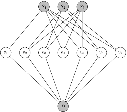
A Simple Multiple Access Network (sman) is defined as follows. A single destination node DD wishes to receive information from multiple source nodes 𝒮={S1,S2,…,S|𝒮|}\mathcal{S}=\left\{S_{1},S_{2},\dots,S_{|\mathcal{S}|}\right\} via a set of intermediate relay nodes 𝒱={v1,…,vN}\mathcal{V}=\left\{v_{1},\ldots,v_{N}\right\}. The information rate of each source Si∈𝒮S_{i}\in\mathcal{S} is denoted by rir_{i}. Each relay node has access to a subset of sources, or equivalently, each source Si∈𝒮S_{i}\in\mathcal{S} is connected to a subset of relay nodes by source links of capacity rir_{i}. Each relay node vi∈𝒱v_{i}\in\mathcal{V} is connected to DD by a link of unit capacity. We refer to these links as relay links. We wish to correct arbitrary or adversarial errors on up to zz relay links or equivalently nodes. An example of a sman is given in Figure 1.

An adjacency matrix 𝐀\mathbf{A} is associated with a sman, where the rows and columns represent 𝒮\mathcal{S} and 𝒱\mathcal{V}, respectively, and 𝐀i,j=1\mathbf{A}_{i,j}=1 if there exists a source link connecting SiS_{i} to vjv_{j}.

Refer to caption
Fig. 1: An example of a sman with 3 sources and 7 intermediate nodes.

Let ℐ⁡(𝒮′)\mathcal{I}(\mathcal{S}^{\prime}) denote the index set of elements in 𝒮′\mathcal{S}^{\prime}, i.e. ℐ⁡(𝒮′)={i:Si∈𝒮′}\mathcal{I}(\mathcal{S}^{\prime})=\left\{i:S_{i}\in\mathcal{S}^{\prime}\right\}. Also define ℐ:=ℐ⁡(𝒮)\mathcal{I}:=\mathcal{I}(\mathcal{S}) and rℐ⁡(𝒮′):=∑i∈ℐ⁡(𝒮′)rir_{\mathcal{I}(\mathcal{S}^{\prime})}:=\sum_{i\in\mathcal{I}(\mathcal{S}^{\prime})}r_{i}. The minimum cut capacity (min-cut) from 𝒮′\mathcal{S}^{\prime} to DD is denoted by Cℐ⁡(𝒮′)C_{\mathcal{I}(\mathcal{S}^{\prime})}, ∀𝒮′⊆𝒮\forall\mathcal{S}^{\prime}\subseteq\mathcal{S}. Note that Cℐ=NC_{\mathcal{I}}=N. From [2], the capacity region ℛ\mathcal{R} of a sman is given by cut set bounds for each subset of sources, i.e. the capacity region is the set of all rate vectors 𝐫=(r1,r2,…,r|𝒮|)\mathbf{r}=\left(r_{1},r_{2},\ldots,r_{|\mathcal{S}|}\right) such that

rℐ⁡(𝒮′)≤Cℐ⁡(𝒮′)−2​z,∀𝒮′⊆𝒮.r_{\mathcal{I}(\mathcal{S}^{\prime})}\leq C_{\mathcal{I}(\mathcal{S}^{\prime})}-2z,\forall\mathcal{S}^{\prime}\subseteq\mathcal{S}.\\ (1)

Furthermore, it suffices to carry out linear network coding at internal network nodes, where each viv_{i} transmits linear combinations of received symbols over 𝔽q\mathbb{F}_{q}.

III Preliminaries

To construct a distributed Reed-Solomon code for the above-described sman with NN intermediate relay nodes and zz adversarial nodes, we start with an [N,k,d]q{\left[N,k,d\right]}_{q} Reed-Solomon code where d=2​z+1=N−k+1d=2z+1=N-k+1. For the purpose of this work, we will use the definition of a Reed-Solomon Code as in [5]. This is a kk-dimensional subspace 𝒞RS={[m(α),m(α2),…,m(αN)]:𝖽𝖾𝗀 m(x)<k}\mathcal{C}_{\text{RS}}=\left\{\left[m(\alpha),m(\alpha^{2}),\ldots,m(\alpha^{N})\right]:\mathsf{deg\text{ }}m(x)<k\right\}, where m⁡(x)m(x) is a polynomial over 𝔽q\mathbb{F}_{q} of degree 𝖽𝖾𝗀 m(x)\mathsf{deg\text{ }}m(x), and α∈𝔽q\alpha\in\mathbb{F}_{q} is a primitive element. The coding scheme operates over a finite field 𝔽q\mathbb{F}_{q}, where qq is a power of a prime pp, such that q≥n+1q\geq n+1. Each message vector 𝐦=[m0,…,mk−1]\mathbf{m}=[m_{0},\ldots,m_{k-1}] is mapped to a message polynomial m⁡(x)=∑i=0k−1mi​xim(x)=\sum_{i=0}^{k-1}m_{i}x^{i}, which is then evaluated at NN distinct elements {α,α,…,αN}\{\alpha,\alpha,\ldots,\alpha^{N}\} of 𝔽q\mathbb{F}_{q}. The vector of evaluations [m⁡(α),m⁡(α2),…,m⁡(αN)]\left[m(\alpha),m(\alpha^{2}),\ldots,m(\alpha^{N})\right] forms the corresponding codeword. This encoding operation can be described concisely using a generator matrix. The generator matrix of 𝒞RS\mathcal{C}_{\text{RS}} is given by 𝐆RS∈𝔽qk×N\mathbf{G}_{\text{RS}}\in\mathbb{F}_{q}^{k\times N}

𝐆RS=[11⋯1αα2⋯αN⋱α(k−1)α2​(k−1)⋯αN⁡(k−1)]\mathbf{G_{\text{RS}}}=\begin{bmatrix}1&1&\cdots&1\\ \alpha&\alpha^{2}&\cdots&\alpha^{N}\\ \vdots&\vdots&\ddots&\vdots\\ \alpha^{(k-1)}&\alpha^{2(k-1)}&\cdots&\alpha^{N(k-1)}\\ \end{bmatrix}

For the convenience of the reader, we restate the BCH Bound which will be used later on. For the proof, see e.g. [6, p.238].

Fact 1 (BCH Bound)

Let p⁡(x)∈𝔽⁡[x]p(x)\in\mathbb{F}[x] be a non-zero polynomial with tt (cyclically) consecutive roots, i.e. p⁡(αj+1)=⋯=p⁡(αj+t)=0p(\alpha^{j+1})=\cdots=p(\alpha^{j+t})=0. Then at least t+1t+1 coefficients of p⁡(x)p(x) are non-zero.

For ease of exposition, and with a slight abuse of terminology, we say that a polynomial p⁡(x)p(x) vanishes on a set 𝒫⊆{1,…,N}\mathcal{P}\subseteq\{1,\ldots,N\} if p⁡(x)=∏i∈𝒫(x−αi)p(x)=\prod_{i\in\mathcal{P}}(x-\alpha^{i}).

IV Code Construction

As mentioned earlier, each relay node in a sman transmits a linear combination of its received symbols. Therefore, the overall coding operation from sources to destination can be represented by a generator matrix 𝐆∈𝔽qrℐ×N\mathbf{G}\in\mathbb{F}_{q}^{r_{\mathcal{I}}\times N}of a specific structure. The structure is captured by 𝐀\mathbf{A}, which is used to build 𝐆\mathbf{G} as follows. We replicate the ithi^{\text{th}} row of 𝐀\mathbf{A} rir_{i} times and then replace the non-zero entries with indeterminates, whose values will be selected later on. We can write 𝐆\mathbf{G} as

𝐆=[𝐆1𝐆2𝐆|𝒮|]\mathbf{G}=\begin{bmatrix}\mathbf{G}_{1}\\ \mathbf{G}_{2}\\ \vdots\\ \mathbf{G}_{|\mathcal{S}|}\end{bmatrix}

where the jjth column of the submatrix 𝐆i∈𝔽qri×N\mathbf{G}_{i}\in\mathbb{F}_{q}^{r_{i}\times N} is all zero if SiS_{i} is not connected to vjv_{j}. For a 3-source sman, 𝐆\mathbf{G} in generic form looks as follows:

𝐆\displaystyle\mathbf{G} =\displaystyle= [𝐆1𝐆2𝐆3]=[×𝟎𝟎𝟎×××𝟎×𝟎×𝟎××𝟎𝟎×××𝟎×]\displaystyle\begin{bmatrix}\mathbf{G}_{1}\\ \mathbf{G}_{2}\\ \mathbf{G}_{3}\end{bmatrix}=\left[\begin{array}[]{c|c|c|c|c|c|c}\bm{\times}&\mathbf{0}&\mathbf{0}&\mathbf{0}&\bm{\times}&\bm{\times}&\bm{\times}\\ \mathbf{0}&\bm{\times}&\mathbf{0}&\bm{\times}&\mathbf{0}&\bm{\times}&\bm{\times}\\ \mathbf{0}&\mathbf{0}&\bm{\times}&\bm{\times}&\bm{\times}&\mathbf{0}&\bm{\times}\\ \end{array}\right]

The symbol ×\times represents a block of indeterminates. For example, the adjacency matrix of the sman in Figure 1 is given by

𝐀=[100111101100110111100]\mathbf{A}=\begin{bmatrix}1&0&0&1&1&1&1\\ 0&1&1&0&0&1&1\\ 0&1&1&1&1&0&0\\ \end{bmatrix}

It should be noted that the permuting the rows and/or columns of 𝐀\mathbf{A} still represents the same network. Thus, we can employ such operations when constructing a code for a certain sman. Now suppose z=1z=1 and 𝐫=(3,1,1)\mathbf{r}=(3,1,1). From 𝐀\mathbf{A}, we build 𝐆\mathbf{G},

𝐆=[g1,100g1,4g1,5g1,6g1,7g2,100g2,4g2,5g2,6g2,7g3,100g3,4g1,5g3,6g3,70g4,2g4,300g4,6g4,70g5,2g5,3g5,4g5,500]\mathbf{G}=\left[\begin{array}[]{ccccccc}g_{1,1}&0&0&g_{1,4}&g_{1,5}&g_{1,6}&g_{1,7}\\ g_{2,1}&0&0&g_{2,4}&g_{2,5}&g_{2,6}&g_{2,7}\\ g_{3,1}&0&0&g_{3,4}&g_{1,5}&g_{3,6}&g_{3,7}\\ \hline\cr 0&g_{4,2}&g_{4,3}&0&0&g_{4,6}&g_{4,7}\\ \hline\cr 0&g_{5,2}&g_{5,3}&g_{5,4}&g_{5,5}&0&0\end{array}\right] (3)

The indeterminates are chosen in way such that the rows of 𝐆\mathbf{G} span an rℐr_{\mathcal{I}}-dimensional subspace 𝒞\mathcal{C} of 𝒞RS\mathcal{C}_{\text{RS}}. We call 𝒞\mathcal{C} a distributed Reed-Solomon code. For each source ii, we can straightforwardly find a basis for the vector space of possible rows of 𝐆i\mathbf{G}_{i} such that it spans an rir_{i}-dimensional subspace of 𝒞RS\mathcal{C}_{\text{RS}}. The only remaining question is whether for any rate vector 𝐫\mathbf{r} in the capacity region it is always possible to find vectors for all 𝐆i\mathbf{G}_{i}’s so that they are collectively linearly independent. We can now describe the encoding operation. Let the message of source SiS_{i} be represented by a row vector 𝐦i=[m1(i),…,mri(i)]\mathbf{m}_{i}=\left[m^{(i)}_{1},\ldots,m^{(i)}_{r_{i}}\right], where mk(i)∈𝔽qm^{(i)}_{k}\in\mathbb{F}_{q}. The jthj^{\text{th}} relay node encodes using the jthj^{\text{th}} column 𝐠(j)\mathbf{g}^{(j)} of the generator matrix 𝐆\mathbf{G}, and transmits the symbol [𝐦1𝐦2…𝐦|𝒮|]​𝐠(j)[\mathbf{m}_{1}\quad\mathbf{m}_{2}\quad\dots\quad\mathbf{m}_{|\mathcal{S}|}]\mathbf{g}^{(j)}. Let 𝐜\mathbf{c} denote the overall network codeword 𝐜=[𝐦1𝐦2…𝐦|𝒮|]​𝐆\mathbf{c}=[\mathbf{m}_{1}\quad\mathbf{m}_{2}\quad\dots\quad\mathbf{m}_{|\mathcal{S}|}]\mathbf{G}. The destination node DD receives a corrupted version of 𝐜\mathbf{c}, denoted by 𝐲=𝐜+𝐞\mathbf{y}=\mathbf{c}+\mathbf{e}, where 𝐞\mathbf{e} is zz-sparse, and yiy_{i} is the symbol received by DD through the ithi^{\text{th}} relay link. The following theorem establishes that this is indeed the case for up to three sources.

Theorem 1

For any rate vector 𝐫∈ℛ\mathbf{r\in\mathcal{R}} in the capacity region of a three-source sman, we can construct a distributed Reed-Solomon code.

The proof is constructive, i.e. for a given sman along with zz, 𝐫\mathbf{r} and 𝐀\mathbf{A}, we show how to find a transformation matrix 𝐓∈𝔽qrℐ×k\mathbf{T}\in\mathbb{F}_{q}^{r_{\mathcal{I}}\times k} such that 𝐆=𝐓𝐆RS\mathbf{G}=\mathbf{T}\mathbf{G}_{\text{RS}}. We can also partition 𝐓\mathbf{T} such that 𝐆i=𝐓i​𝐆RS\mathbf{G}_{i}=\mathbf{T}_{i}\mathbf{G}_{\text{RS}}:

𝐓=[𝐓1𝐓2𝐓|𝒮|]\mathbf{T}=\begin{bmatrix}\mathbf{T}_{1}\\ \mathbf{T}_{2}\\ \vdots\\ \mathbf{T}_{|\mathcal{S}|}\end{bmatrix}

We prove that such a construction is possible by considering four possible cases. Any sman with 𝐫∈ℛ\mathbf{r}\in\mathcal{R} falls precisely under one of these cases. For the first three cases, we show that it is always possible to set the indeterminates in a way such that rir_{i} columns in 𝐆i\mathbf{G}_{i} form an upper triangular matrix, guaranteeing 𝗋𝖺𝗇𝗄⁡(𝐆)=ri\mathsf{rank}(\mathbf{G})=r_{i}. Given the structure of 𝐆RS\mathbf{G}_{\text{RS}}, we can exactly describe 𝐓\mathbf{T} by resorting to a polynomial representation of vectors. Effectively, we transform 𝐆RS\mathbf{G}_{\text{RS}} into a matrix in row echelon form (up to a permutation of the columns). The fourth case relies on a different strategy, which is treated in a self-contained fashion. We now introduce some needed notation. For all 𝒮′⊆𝒮\mathcal{S}^{\prime}\subseteq\mathcal{S}, let 𝒩ℐ⁡(𝒮′)∈ℐ⁡(𝒱)\mathcal{N}_{\mathcal{I}(\mathcal{S}^{\prime})}\in\mathcal{I}(\mathcal{V}) denote the set of column indices corresponding to intermediate nodes connected to all Si∈𝒮′S_{i}\in\mathcal{S}^{\prime} simultaneously, but not to any other source. We say 𝒩ℐ⁡(𝒮′)\mathcal{N}_{\mathcal{I}(\mathcal{S}^{\prime})} represents the columns indexed by its elements. Let nℐ⁡(𝒮′):=|𝒩ℐ⁡(𝒮′)|n_{\mathcal{I}(\mathcal{S}^{\prime})}:=|\mathcal{N}_{\mathcal{I}(\mathcal{S}^{\prime})}|. For the network in Figure 1, 𝒩1={1}\mathcal{N}_{1}=\left\{1\right\}, and 𝒩1,2={6,7}\mathcal{N}_{1,2}=\left\{6,7\right\}. Note that the sets 𝒩𝒮′\mathcal{N}_{\mathcal{S}^{\prime}} partition ℐ⁡(𝒱)\mathcal{I}(\mathcal{V}). Let 𝒵i\mathcal{Z}_{i} be the set of indices of the columns corresponding to the relay nodes that are not connected to SiS_{i}. For example, 𝒵2={1,4,5}\mathcal{Z}_{2}=\{1,4,5\}. We will say that 𝒳⊆𝒩ℐ⁡(𝒮′)\mathcal{X}\subseteq\mathcal{N}_{\mathcal{I}(\mathcal{S}^{\prime})} is contained in the set of roots of a polynomial p⁡(x)p(x) if p⁡(αi)=0p(\alpha^{i})=0 for all i∈𝒳i\in\mathcal{X}. We now prove the main theorem by considering each of the following four cases.

Case 1

r1\displaystyle r_{1} ≤\displaystyle\leq n1\displaystyle n_{1} (4)
r2\displaystyle r_{2} ≤\displaystyle\leq n2+n1,2\displaystyle n_{2}+n_{1,2} (5)

Without loss of generality, we assume

𝒩1\displaystyle\mathcal{N}_{1} =\displaystyle= {1,…,n1}\displaystyle\{1,\ldots,n_{1}\}
𝒩2\displaystyle\mathcal{N}_{2} =\displaystyle= {n1+1,…,n1+n2}\displaystyle\{n_{1}+1,\ldots,n_{1}+n_{2}\}
𝒩1,2\displaystyle\mathcal{N}_{1,2} =\displaystyle= {n1+n2+1,…,n1+n2+n1,2}\displaystyle\{n_{1}+n_{2}+1,\ldots,n_{1}+n_{2}+n_{1,2}\}

Given the constraint on r1r_{1} in (4), we can select r1r_{1} columns represented by a subset of 𝒩1\mathcal{N}_{1} in 𝐆1\mathbf{G}_{1} and set as the identity matrix (or any other diagonal matrix). Similarly by (5), a collection of r2r_{2} columns represented by a subset of 𝒩2∪𝒩1,2\mathcal{N}_{2}\cup\mathcal{N}_{1,2} in 𝐆2\mathbf{G}_{2} is set as a diagonal matrix. We now move to on to 𝐆3\mathbf{G}_{3} and select any r3r_{3} columns to set as a diagonal matrix. In essence, the indeterminates of 𝐆\mathbf{G} are chosen such that it is in row echelon form (up to a permutation of the columns). To show that such matrix can constructed from 𝐆RS\mathbf{G}_{\text{RS}}, we define the rows of 𝐓\mathbf{T} as polynomials that vanish on appropriate sets and have the appropriate degree. Let tj(1)​(x)t^{(1)}_{j}(x) be a polynomial that vanishes on 𝒵1∪{1,…,r1}∖j\mathcal{Z}_{1}\cup\{1,\ldots,r_{1}\}\setminus j. The jthj^{\text{th}} row of 𝐓1\mathbf{T}_{1} is the vector of coefficients of tj(1)​(x)t^{(1)}_{j}(x) along with extra zeros so that it is composed of kk entries. Now, let tj(2)​(x)t^{(2)}_{j}(x) be a polynomial that vanishes on 𝒵2∪{n1+1,…,n1+r2}∖(n1+j)\mathcal{Z}_{2}\cup\{n_{1}+1,\ldots,n_{1}+r_{2}\}\setminus\left(n_{1}+j\right). 𝐓2\mathbf{T}_{2} is built in the same manner as 𝐓1\mathbf{T}_{1}. To build 𝐓3\mathbf{T}_{3}, choose tj(3)​(x)t^{(3)}_{j}(x) such that it vanishes on 𝒵3∪{n1+n2+n1,2+1,…,n1+n2+n1,2+r3}∖(n1+n2+n1,2+j)\mathcal{Z}_{3}\cup\{n_{1}+n_{2}+n_{1,2}+1,\ldots,n_{1}+n_{2}+n_{1,2}+r_{3}\}\setminus\left(n_{1}+n_{2}+n_{1,2}+j\right). Using this method, we transform 𝐆RS\mathbf{G}_{\text{RS}} into 𝐆\mathbf{G}, which is in row echelon form and has no all-zero rows. The cut-set bounds (1) along with the number of roots of tj(i)​(x)t_{j}^{(i)}(x) imply 𝖽𝖾𝗀 tj(i)(x)≤k−1\mathsf{deg\text{ }}t_{j}^{(i)}(x)\leq k-1. To see this, consider tj(1)​(x)t_{j}^{(1)}{(x)} first, which has |𝒵1|+r1−1|\mathcal{Z}_{1}|+r_{1}-1 roots. Since r1≤C1−2​zr_{1}\leq C_{1}-2z and |𝒵1|=N−C1|\mathcal{Z}_{1}|=N-C_{1}, we have |𝒵1|+r1−1≤N−2​z−1=k−1|\mathcal{Z}_{1}|+r_{1}-1\leq N-2z-1=k-1. The same argument justifies the claim for tj(2)​(x)t_{j}^{(2)}(x) and tj(3)​(x)t_{j}^{(3)}(x). Thus, an appropriate 𝐓\mathbf{T} can always be found and 𝗋𝖺𝗇𝗄⁡(𝐆)=Rℐ\mathsf{rank}(\mathbf{G})=R_{\mathcal{I}}, as required.

Case 2

r1\displaystyle r_{1} ≤\displaystyle\leq n1\displaystyle n_{1}
r2\displaystyle r_{2} >\displaystyle> n2+n1,2\displaystyle n_{2}+n_{1,2}

We make the same assumptions on 𝒩1\mathcal{N}_{1}, 𝒩2\mathcal{N}_{2} and 𝒩1,2\mathcal{N}_{1,2}. Furthermore,

𝒩2,3\displaystyle\mathcal{N}_{2,3} =\displaystyle= {n1+n2+n1,2+1,…,n1+n2+n1,2+n2,3}\displaystyle\{n_{1}+n_{2}+n_{1,2}+1,\ldots,n_{1}+n_{2}+n_{1,2}+n_{2,3}\}
𝒩1,2,3\displaystyle\mathcal{N}_{1,2,3} =\displaystyle= {n1+n2+n1,2+n2,3+1,…,n1+n2+n1,2+n2,3+n1,2,3}\displaystyle\{n_{1}+n_{2}+n_{1,2}+n_{2,3}+1,\ldots,n_{1}+n_{2}+n_{1,2}+n_{2,3}+n_{1,2,3}\}

We define tj(1)​(x)t^{(1)}_{j}(x) and tj(2)​(x)t^{(2)}_{j}(x) as in Case 1. Since r2>n2+n1,2r_{2}>n_{2}+n_{1,2}, 𝐓2\mathbf{T}_{2} will affect, in addition to 𝒩2∪𝒩1,2\mathcal{N}_{2}\cup\mathcal{N}_{1,2} columns represented by 𝒳(2)=𝒳2,3(2)∪𝒳1,2,3(2)\mathcal{X}^{\left(2\right)}=\mathcal{X}^{\left(2\right)}_{2,3}\cup\mathcal{X}^{\left(2\right)}_{1,2,3}, where 𝒳2,3(2)⊆𝒩2,3\mathcal{X}^{\left(2\right)}_{2,3}\subseteq\mathcal{N}_{2,3} and 𝒳1,2,3(2)⊆𝒩1,2,3\mathcal{X}^{\left(2\right)}_{1,2,3}\subseteq\mathcal{N}_{1,2,3}, and x2:=|𝒳(2)|=r2−(n2+n1,2)x_{2}:=|\mathcal{X}^{\left(2\right)}|=r_{2}-(n_{2}+n_{1,2}). In other words, 𝒳2,3(2)\mathcal{X}^{\left(2\right)}_{2,3} is the subset of 𝒩2,3\mathcal{N}_{2,3} contained in ∪jℒj\cup_{j}{\cal{L}}_{j}, where ℒj{\cal{L}}_{j} is the set of roots of tj(2)​(x)t_{j}^{(2)}(x). In order to have 𝐆\mathbf{G} in row echelon form, we need to modify tj(3)​(x)t^{(3)}_{j}(x) such that 𝐓3\mathbf{T}_{3} also sets the indeterminates in the columns represented by 𝒳(2)\mathcal{X}^{\left(2\right)} in 𝐆3\mathbf{G}_{3} to zero. Namely, tj(3)​(x)t^{(3)}_{j}(x) vanishes on 𝒳(2)∪𝒵3∪{n1+n2+n1,2+x2+1,…,n1+n2+n1,2+x2+r3}∖n1+n2+n1,2+x2+j\mathcal{X}^{\left(2\right)}\cup\mathcal{Z}_{3}\cup\{n_{1}+n_{2}+n_{1,2}+x_{2}+1,\ldots,n_{1}+n_{2}+n_{1,2}+x_{2}+r_{3}\}\setminus n_{1}+n_{2}+n_{1,2}+x_{2}+j. Since tj(1)​(x)t_{j}^{(1)}(x) and tj(2)​(x)t_{j}^{(2)}(x) are chosen as in Case 1, their degrees are at most k−1k-1 as required. For tj(3)​(x)t_{j}^{(3)}(x), the following relations give the required results:

𝖽𝖾𝗀 tj(3)(x)\displaystyle\mathsf{deg\text{ }}t_{j}^{(3)}(x) =\displaystyle= |𝒵3|+x2+r3−1\displaystyle|\mathcal{Z}_{3}|+x_{2}+r_{3}-1
=\displaystyle= N−C3+r2−n2−n1,2+r3−1\displaystyle N-C_{3}+r_{2}-n_{2}-n_{1,2}+r_{3}-1
=\displaystyle= n1+r2+r3−1\displaystyle n_{1}+r_{2}+r_{3}-1
≤\displaystyle\leq n1+C2,3−2​z−1\displaystyle n_{1}+C_{2,3}-2z-1
=\displaystyle= N−2​z−1\displaystyle N-2z-1
=\displaystyle= k−1\displaystyle k-1

Case 3

r1\displaystyle r_{1} >\displaystyle> n1\displaystyle n_{1} (6)
r2\displaystyle r_{2} >\displaystyle> n2+n1,2\displaystyle n_{2}+n_{1,2} (7)

Assume that the elements of the index set ℐ⁡(𝒱)\mathcal{I}(\mathcal{V}) are ordered as follows: 𝒩1,𝒩1,3,𝒩2,𝒩1,2,𝒩2,3,𝒩3,𝒩1,2,3\mathcal{N}_{1},\mathcal{N}_{1,3},\mathcal{N}_{2},\mathcal{N}_{1,2},\mathcal{N}_{2,3},\mathcal{N}_{3},\mathcal{N}_{1,2,3}. Given this ordering, the set 𝒩1,2\mathcal{N}_{1,2} will be used when constructing 𝐆2\mathbf{G}_{2}. Furthemore, the columns represented by 𝒩1,3\mathcal{N}_{1,3} are exhausted in preference to 𝒩1,2,3\mathcal{N}_{1,2,3} when constructing 𝐓1\mathbf{T}_{1}. In other words, the set of roots of tj(1)​(x)t_{j}^{(1)}(x) will contain (a subset of) 𝒩1,2,3\mathcal{N}_{1,2,3} only if r1−(n1+n1,3)>0r_{1}-(n_{1}+n_{1,3})>0. For 𝐓2\mathbf{T}_{2}, a similar reasoning holds by preferring 𝒩2,3\mathcal{N}_{2,3} over 𝒩1,2,3\mathcal{N}_{1,2,3}. Our intuition for such ordering is that it utilizes already present zeros in 𝐆\mathbf{G} to contribute to 𝗋𝖺𝗇𝗄⁡(𝐆)\mathsf{rank}(\mathbf{G}). As before, tj(1)​(x)t_{j}^{(1)}(x) vanishes on 𝒵1∪{i1,…,ir1}∖ij\mathcal{Z}_{1}\cup\{i_{1},\ldots,i_{r_{1}}\}\setminus i_{j}, where ili_{l} is the lthl^{\text{th}} element in the ordered set ℐ⁡(𝒱)∖{𝒵1∪𝒩1,2}\mathcal{I}(\mathcal{V})\setminus\{\mathcal{Z}_{1}\cup\mathcal{N}_{1,2}\}. Note that (7) implies that the set of roots of tj(2)​(x)t_{j}^{(2)}(x) contains 𝒩1,2\mathcal{N}_{1,2}. Similarly, tj(2)​(x)t_{j}^{(2)}(x) vanishes on 𝒳1,2,3(1)∪𝒵2∪{i1,…,ir2}∖ij\mathcal{X}^{\left(1\right)}_{1,2,3}\cup\mathcal{Z}_{2}\cup\{i_{1},\ldots,i_{r_{2}}\}\setminus i_{j}, where ili_{l} is the lthl^{\text{th}} element in the ordered set 𝒵2¯∖𝒳1,2,3(1)\bar{\mathcal{Z}_{2}}\setminus\mathcal{X}^{\left(1\right)}_{1,2,3}. Lastly, tj(3)​(x)t_{j}^{(3)}(x) vanishes on 𝒳1,2,3(1)∪𝒳1,2,3(2)∪𝒳1,3(1)∪𝒳2,3(2)∪𝒵3∪{i1,…,ir3}∖ij\mathcal{X}^{\left(1\right)}_{1,2,3}\cup\mathcal{X}^{\left(2\right)}_{1,2,3}\cup\mathcal{X}^{\left(1\right)}_{1,3}\cup\mathcal{X}^{\left(2\right)}_{2,3}\cup\mathcal{Z}_{3}\cup\{i_{1},\ldots,i_{r_{3}}\}\setminus i_{j} and ili_{l} is the lthl^{\text{th}} element in the ordered set 𝒵3¯∖(𝒳1,2,3(1)∪𝒳1,2,3(2)∪𝒳1,3(1)∪𝒳2,3(2))\bar{\mathcal{Z}_{3}}\setminus(\mathcal{X}^{\left(1\right)}_{1,2,3}\cup\mathcal{X}^{\left(2\right)}_{1,2,3}\cup\mathcal{X}^{\left(1\right)}_{1,3}\cup\mathcal{X}^{\left(2\right)}_{2,3}). Before validating our choice of tj(i)​(x)t_{j}^{(i)}(x), we characterize the sizes of 𝒳1,3(1),𝒳2,3(2),𝒳1,2,3(1),𝒳1,2,3(2)\mathcal{X}^{\left(1\right)}_{1,3},\mathcal{X}^{\left(2\right)}_{2,3},\mathcal{X}^{\left(1\right)}_{1,2,3},\mathcal{X}^{\left(2\right)}_{1,2,3}:

|𝒳1,3(1)|\displaystyle\left|\mathcal{X}^{\left(1\right)}_{1,3}\right| =\displaystyle= 𝗆𝗂𝗇⁡(n1,3,r1−n1)\displaystyle\mathsf{min}(n_{1,3},r_{1}-n_{1})
|𝒳2,3(2)|\displaystyle|\mathcal{X}^{\left(2\right)}_{2,3}| =\displaystyle= 𝗆𝗂𝗇⁡(n2,3,r2−(n2+n1,2))\displaystyle\mathsf{min}(n_{2,3},r_{2}-(n_{2}+n_{1,2}))
|𝒳1,2,3(1)|\displaystyle|\mathcal{X}^{\left(1\right)}_{1,2,3}| =\displaystyle= r1−n1−|𝒳1,3(1)|\displaystyle r_{1}-n_{1}-|\mathcal{X}^{\left(1\right)}_{1,3}|
|𝒳1,2,3(2)|\displaystyle|\mathcal{X}^{\left(2\right)}_{1,2,3}| =\displaystyle= r2−(n2+n1,2)−|𝒳2,3(2)|\displaystyle r_{2}-(n_{2}+n_{1,2})-|\mathcal{X}^{\left(2\right)}_{2,3}|

We now bound the degree of tj(i)​(x)t_{j}^{(i)}(x). Using the same argument as in Case 1, 𝖽𝖾𝗀 tj(1)(x)≤k−1\mathsf{deg\text{ }}t_{j}^{(1)}(x)\leq k-1. Now we consider tj(2)​(x)t_{j}^{(2)}(x). Assume |𝒳1,3(1)|=n1,3\left|\mathcal{X}^{\left(1\right)}_{1,3}\right|=n_{1,3}:

𝖽𝖾𝗀 tj(2)(x)\displaystyle\mathsf{deg\text{ }}t_{j}^{(2)}(x) =\displaystyle= |𝒳1,2,3(1)|+|𝒵2|+r2−1\displaystyle|\mathcal{X}^{\left(1\right)}_{1,2,3}|+|\mathcal{Z}_{2}|+r_{2}-1
=\displaystyle= r1−n1−n1,3+N−C2+r2−1\displaystyle r_{1}-n_{1}-n_{1,3}+N-C_{2}+r_{2}-1
=\displaystyle= r1+r2+n3−1\displaystyle r_{1}+r_{2}+n_{3}-1
≤\displaystyle\leq C1,2−2​z+n3−1\displaystyle C_{1,2}-2z+n_{3}-1
=\displaystyle= k−1\displaystyle k-1

The same approach holds when justifying the claim for tj(3)​(x)t_{j}^{(3)}(x). What remains to show is that |𝒳1,2,3(1)|+|𝒳1,2,3(2)|≤n1,2,3|\mathcal{X}^{\left(1\right)}_{1,2,3}|+|\mathcal{X}^{\left(2\right)}_{1,2,3}|\leq n_{1,2,3}. Assume |𝒳1,2,3(1)|=r1−n1−n1,3|\mathcal{X}^{\left(1\right)}_{1,2,3}|=r_{1}-n_{1}-n_{1,3}, |𝒳1,2,3(2)|=r2−(n2+n1,2)−n2,3|\mathcal{X}^{\left(2\right)}_{1,2,3}|=r_{2}-(n_{2}+n_{1,2})-n_{2,3}. This is justified since columns represented by elements in 𝒩1,2,3\mathcal{N}_{1,2,3} are used in the construction of 𝐆1\mathbf{G}_{1} and 𝐆2\mathbf{G}_{2} only if these assumptions hold. By assumption on 𝐫\mathbf{r}, r1+r2≤C1,2−2​z≤C1,2=n1+n2+n1,2+n1,3+n2,3+n1,2,3r_{1}+r_{2}\leq C_{1,2}-2z\leq C_{1,2}=n_{1}+n_{2}+n_{1,2}+n_{1,3}+n_{2,3}+n_{1,2,3}. Rearranging this to r1−n1−n1,3+r2−(n2+n1,2)−n2,3≤n1,2,3r_{1}-n_{1}-n_{1,3}+r_{2}-(n_{2}+n_{1,2})-n_{2,3}\leq n_{1,2,3} and noticing that the left hand side of the inequality is equal to |𝒳1,2,3(1)|+|𝒳1,2,3(2)||\mathcal{X}^{\left(1\right)}_{1,2,3}|+|\mathcal{X}^{\left(2\right)}_{1,2,3}| yields the result.

Case 4

r1\displaystyle r_{1} >\displaystyle> n1\displaystyle n_{1}
r2\displaystyle r_{2} ≤\displaystyle\leq n2+n1,2\displaystyle n_{2}+n_{1,2}

This case is approached differently. First, we permute the 𝐆i\mathbf{G}_{i}’s to recast the problem such that it falls under Case 1, 2 or 3. If this is possible, then we basically construct the code as earlier. Otherwise, for all i≠ji\neq j,

ri\displaystyle r_{i} >\displaystyle> ni\displaystyle n_{i} (8)
ri\displaystyle r_{i} ≤\displaystyle\leq ni+ni,j\displaystyle n_{i}+n_{i,j} (9)

We will assume that the columns of 𝐆\mathbf{G} are ordered in the following manner.

𝐆=[𝐆1𝐆2𝐆3]=[×𝟎𝟎××𝟎×𝟎×𝟎×𝟎××𝟎𝟎×𝟎×××]\mathbf{G}=\begin{bmatrix}\mathbf{G}_{1}\\ \mathbf{G}_{2}\\ \mathbf{G}_{3}\end{bmatrix}=\left[\begin{array}[]{ccc|ccc|c}\bm{\times}&\mathbf{0}&\mathbf{0}&\bm{\times}&\bm{\times}&\mathbf{0}&\bm{\times}\\ \mathbf{0}&\bm{\times}&\mathbf{0}&\bm{\times}&\mathbf{0}&\bm{\times}&\bm{\times}\\ \mathbf{0}&\mathbf{0}&\bm{\times}&\mathbf{0}&\bm{\times}&\bm{\times}&\bm{\times}\\ \end{array}\right]

For this case, we place an identity of size nin_{i} in the submatrix that corresponds to the columns represented by 𝒩i\mathcal{N}_{i} and the block 𝐆i\mathbf{G}_{i}. We permute the rows of 𝐆\mathbf{G} to obtain the following:

𝐆=[𝐈𝟎𝟎××𝟎×𝟎𝐈𝟎×𝟎××𝟎𝟎𝐈𝟎×××𝟎𝟎𝟎××𝟎×𝟎𝟎𝟎×𝟎××𝟎𝟎𝟎𝟎×××]\mathbf{G}=\left[\begin{array}[]{ccc|ccc|c}\mathbf{I}&\mathbf{0}&\mathbf{0}&\bm{\times}&\bm{\times}&\mathbf{0}&\bm{\times}\\ \mathbf{0}&\mathbf{I}&\mathbf{0}&\bm{\times}&\mathbf{0}&\bm{\times}&\bm{\times}\\ \mathbf{0}&\mathbf{0}&\mathbf{I}&\mathbf{0}&\bm{\times}&\bm{\times}&\bm{\times}\\ \hline\cr\mathbf{0}&\mathbf{0}&\mathbf{0}&\bm{\times}&\bm{\times}&\mathbf{0}&\bm{\times}\\ \mathbf{0}&\mathbf{0}&\mathbf{0}&\bm{\times}&\mathbf{0}&\bm{\times}&\bm{\times}\\ \mathbf{0}&\mathbf{0}&\mathbf{0}&\mathbf{0}&\bm{\times}&\bm{\times}&\bm{\times}\\ \end{array}\right] (10)

The blocks of columns of 𝐆\mathbf{G} have sizes n1,n2,n3,n1,2,n1,3,n2,3,n1,2,3n_{1},n_{2},n_{3},n_{1,2},n_{1,3},n_{2,3},n_{1,2,3}, while the blocks of rows have sizes n1,n2,n3,r1−n1,r2−n2,r3−n3n_{1},n_{2},n_{3},r_{1}-n_{1},r_{2}-n_{2},r_{3}-n_{3}.

We will construct a matrix 𝐓\mathbf{T} (with dimensions Rℐ×kR_{\mathcal{I}}\times k), partitioned into two row-blocks, that will transform the generator matrix of a [N,k,d]\left[N,k,d\right] RS code 𝐆RS\mathbf{G}_{\text{RS}} to one whose mask is given by 𝐆\mathbf{G} in (10).

𝐆=𝐓𝐆RS=[𝐒𝐕]​𝐆RS=[𝐈𝐆^𝟏𝟎𝐆^𝟐]=[𝐗𝐆^]\mathbf{G}=\mathbf{T}\mathbf{G}_{\text{RS}}=\begin{bmatrix}\mathbf{S}\\ \mathbf{V}\end{bmatrix}\mathbf{G}_{\text{RS}}=\left[\begin{array}[]{c|c}\mathbf{I}&\mathbf{\hat{G}_{1}}\\ \hline\cr\mathbf{0}&\mathbf{\hat{G}_{2}}\\ \end{array}\right]=\begin{bmatrix}\mathbf{X}\\ \hat{\mathbf{G}}\\ \end{bmatrix} (11)

Note that 𝐒\mathbf{S} has n¯:=∑ni\bar{n}:=\sum n_{i} rows and 𝐕\mathbf{V} has R′:=∑ri′R^{\prime}:=\sum r^{\prime}_{i} rows, where ri′=ri−nir_{i}^{\prime}=r_{i}-n_{i}. Constructing 𝐒\mathbf{S} is straightforward and we only focus on 𝐕\mathbf{V}.

Construction of 𝐕\mathbf{V}

As before, the construction boils down to finding polynomials with the appropriate roots, i.e. roots corresponding to the zeros in 𝐆^\hat{\mathbf{G}}. Each of these polynomials will have N−(1+2​z)N-(1+2z) roots. Using the coefficients of these polynomials as the rows of 𝐕\mathbf{V} will provide the required result. Let c⁡(x)=∏i=1n¯(x−αi)c(x)=\prod_{i=1}^{\bar{n}}(x-\alpha^{i}). This polynomial will produce the all-zero columns of 𝐆^\hat{\mathbf{G}}, namely the columns represented by 𝒩1∪𝒩2∪𝒩3\mathcal{N}_{1}\cup\mathcal{N}_{2}\cup\mathcal{N}_{3}. Now consider the polynomial p⁡(x)=∏i∈𝒫(x−αi)p(x)=\prod_{i\in\mathcal{P}}(x-\alpha^{i}) which vanishes on 𝒫={n1,2+n1,3+n¯+1,n1,2+n1,3+n¯+2,…,n1,2+n1,3+k−1}\mathcal{P}=\{n_{1,2}+n_{1,3}+\bar{n}+1,n_{1,2}+n_{1,3}+\bar{n}+2,\ldots,n_{1,2}+n_{1,3}+k-1\}, and form the polynomial v⁡(x)=c⁡(x)​p​(x)v(x)=c(x)p(x). Defining the row vector [v⁡(αi)][v(\alpha^{i})], i=1,…,Ni=1,\ldots,N yields the first row of 𝐆^\hat{\mathbf{G}} in (11).

To proceed with the construction,we define the following sets:

𝒥1\displaystyle\mathcal{J}_{1} =\displaystyle= {0,1,…,r1′−1}\displaystyle\left\{0,1,\ldots,r^{\prime}_{1}-1\right\}
𝒥2\displaystyle\mathcal{J}_{2} =\displaystyle= {n1,3,n1,3+1,…,n1,3+r2′−1}\displaystyle\left\{n_{1,3},n_{1,3}+1,\ldots,n_{1,3}+r^{\prime}_{2}-1\right\}
𝒥3\displaystyle\mathcal{J}_{3} =\displaystyle= {n1,3+n1,2,n1,3+n1,2+1,…,n1,3+n1,2+r3′−1}\displaystyle\left\{n_{1,3}+n_{1,2},n_{1,3}+n_{1,2}+1,\ldots,n_{1,3}+n_{1,2}+r^{\prime}_{3}-1\right\}

We partition 𝐕\mathbf{V} as follows:

𝐕=[𝐕1𝐕2𝐕3]\mathbf{V}=\begin{bmatrix}\mathbf{V}_{1}\\ \mathbf{V}_{2}\\ \mathbf{V}_{3}\end{bmatrix}

The jthj^{\text{th}} row of 𝐕i\mathbf{V}_{i} (with dimensions ri′×kr^{\prime}_{i}\times k) corresponds to the coefficients of vj(i)​(x)=c⁡(x)​p​(αj​x)v^{(i)}_{j}(x)=c(x)p(\alpha^{j}x), where j∈𝒥ij\in\mathcal{J}_{i}. Using this method, c⁡(x)c(x) still produces the zeros required for the all zero block. The remaining zeros in each row are produced by p⁡(αj​x)p(\alpha^{j}x), which basically shifts the location of the roots of p⁡(x)p(x) by jj positions to the left appropriately. Since p⁡(x)p(x) has t=k−n¯−1t=k-\bar{n}-1 roots, a row in 𝐆^2\hat{\mathbf{G}}_{2} with a requirement of, say, n2,3n_{2,3} zeros will have an excess of t−n2,3t-n_{2,3} zeros. Nonetheless, the weight of every row of 𝐆^\hat{\mathbf{G}} is still at least 1+2​z1+2z. Now, we proceed to show that 𝐕\mathbf{V} is full rank.

First, we need that the 𝒥1,𝒥2,𝒥3\mathcal{J}_{1},\mathcal{J}_{2},\mathcal{J}_{3} sets are pairwise disjoint. Note the elements in each 𝒥i\mathcal{J}_{i} are increasing. By the constraints (9), r1≤n1+n1,3r_{1}\leq n_{1}+n_{1,3}. Thus r1′−1<n1,3r^{\prime}_{1}-1<n_{1,3} and 𝒥1∩𝒥2=∅\mathcal{J}_{1}\cap\mathcal{J}_{2}=\emptyset. A similar argument implies 𝒥2∩𝒥3=∅\mathcal{J}_{2}\cap\mathcal{J}_{3}=\emptyset.

Now, we show that the polynomials vj(i)​(x)v^{(i)}_{j}(x) are linearly independent. Note that this is true if and only if the polynomials p⁡(αj​x)p(\alpha^{j}x) are linearly independent. Therefore, we focus on the latter.

V Rank of 𝐕\mathbf{V}

Write p⁡(x)=∑l=0tpl​xlp(x)=\sum_{l=0}^{t}p_{l}x^{l} and p⁡(αj​x)=∑l=0tpl​αj​l​xlp(\alpha^{j}x)=\sum_{l=0}^{t}p_{l}\alpha^{jl}x^{l}. Consider the matrix 𝐏\mathbf{P} formed by the coefficients of p⁡(αj​x)p(\alpha^{j}x), j∈∪i𝒥ij\in\cup_{i}\mathcal{J}_{i}

𝐏=[p0p1​αj1…pt​αj1​tp0p1​αj2…pt​αj2​t⋱p0p1​αjR′…pt​αjR′​t]\mathbf{P}=\begin{bmatrix}p_{0}&p_{1}\alpha^{j_{1}}&\ldots&p_{t}\alpha^{j_{1}t}\\ p_{0}&p_{1}\alpha^{j_{2}}&\ldots&p_{t}\alpha^{j_{2}t}\\ \vdots&\vdots&\ddots&\vdots\\ p_{0}&p_{1}\alpha^{j_{R^{\prime}}}&\ldots&p_{t}\alpha^{j_{R^{\prime}}t}\\ \end{bmatrix}

The matrix 𝐏\mathbf{P} (dimensions R′×t+1R^{\prime}\times t+1) is never a tall matrix since by the rate region R′≤t+1R^{\prime}\leq t+1. Consider the matrix 𝐏^\hat{\mathbf{P}} which is formed from the first R′R^{\prime} columns of 𝐏\mathbf{P}. Writing out the determinant of 𝐏^\hat{\mathbf{P}} yields

𝖽𝖾𝗍⁡(𝐏^)\displaystyle\mathsf{det}(\hat{\mathbf{P}}) =\displaystyle= |p0p1​αj1…pR−1​αj1​(R′−1)p0p1​αj2…pR−1​αj2​(R′−1)⋱p0p1​αjR′…pR′−1​αjR′​(R′−1)|\displaystyle\begin{vmatrix}p_{0}&p_{1}\alpha^{j_{1}}&\ldots&p_{R-1}\alpha^{j_{1}(R^{\prime}-1)}\\ p_{0}&p_{1}\alpha^{j_{2}}&\ldots&p_{R-1}\alpha^{j_{2}(R^{\prime}-1)}\\ \vdots&\vdots&\ddots&\vdots\\ p_{0}&p_{1}\alpha^{j_{R^{\prime}}}&\ldots&p_{R^{\prime}-1}\alpha^{j_{R^{\prime}}(R^{\prime}-1)}\\ \end{vmatrix}
=\displaystyle= ∏i=0R′−1pi​|1αj1…αj1​(R′−1)1αj2…αj2​(R′−1)⋱1αjR′…αjR′​(R′−1)|\displaystyle\prod_{i=0}^{R^{\prime}-1}p_{i}\begin{vmatrix}1&\alpha^{j_{1}}&\ldots&\alpha^{j_{1}(R^{\prime}-1)}\\ 1&\alpha^{j_{2}}&\ldots&\alpha^{j_{2}(R^{\prime}-1)}\\ \vdots&\vdots&\ddots&\vdots\\ 1&\alpha^{j_{R^{\prime}}}&\ldots&\alpha^{j_{R^{\prime}}(R^{\prime}-1)}\\ \end{vmatrix}

Using the BCH bound, we establish that all pip_{i}’s are nonzero. Therefore 𝖽𝖾𝗍⁡(𝐏^)\mathsf{det}(\hat{\mathbf{P}}) is equal to the determinant of the Vandermonde matrix with defining set {αj1,…,αjR′}\{\alpha^{j_{1}},\ldots,\alpha^{j_{R^{\prime}}}\}, multiplied by a non-zero scalar. As it was established earlier, the elements {αj1,…,αjR′}\{\alpha^{j_{1}},\ldots,\alpha^{j_{R^{\prime}}}\} are all distinct in 𝔽q\mathbb{F}_{q}.

Therefore, 𝐏\mathbf{P} is full rank implying that the polynomials vj(i)​(x)v_{j}^{(i)}(x) are linearly independent and so 𝗋𝖺𝗇𝗄⁡(𝐆^)=R′\mathsf{rank}(\hat{\mathbf{G}})=R^{\prime}. We also observe that 𝗋𝖺𝗇𝗄⁡(𝐆)=𝗋𝖺𝗇𝗄⁡(𝐗)+𝗋𝖺𝗇𝗄⁡(𝐆^)=n¯+R′=Rℐ\mathsf{rank}(\mathbf{G})=\mathsf{rank}(\mathbf{X})+\mathsf{rank}(\hat{\mathbf{G}})=\bar{n}+R^{\prime}=R_{\mathcal{I}}. Thus 𝐆\mathbf{G} is full rank.

VI Decoding Details

In essence, we have used a subcode of a RS code to correct errors in a sman. Generally speaking, any decoding algorithm designed for evaluation-based construction of RS-codes can be used to decode the received symbols to a valid codeword 𝐜^\hat{\mathbf{c}}. However, this doesn’t imply that the we can immediately de-map the codeword to the original message 𝐦\mathbf{m}. Nonetheless, if we were to use a decoder that produces a valid message 𝐦^RS\hat{\mathbf{m}}_{\text{RS}} such that 𝐜^=𝐦^RS​𝐆RS\hat{\mathbf{c}}=\hat{\mathbf{m}}_{\text{RS}}\mathbf{G}_{\text{RS}}, then we can obtain an estimate of the transmitted message vector 𝐦^\hat{\mathbf{m}} easily using our knowledge of 𝐓\mathbf{T}.

Thus, we use the Berlekamp-Welch decoder as described by Gemmell and Sudan in [7]. Assuming at most zz errors occur, we recover the unique 𝐦RS\mathbf{m}_{\text{RS}} such that 𝐜=𝐦𝐆=𝐦𝐓𝐆RS=𝐦RS​𝐆RS\mathbf{c}=\mathbf{m}\mathbf{G}=\mathbf{m}\mathbf{T}\mathbf{G}_{\text{RS}}=\mathbf{m}_{\text{RS}}\mathbf{G}_{\text{RS}}. Since 𝐓\mathbf{T} has full row rank, it follows that 𝐦RS=𝐦𝐓\mathbf{m}_{\text{RS}}=\mathbf{m}\mathbf{T}. Next let 𝐓~\tilde{\mathbf{T}} be a matrix of RℐR_{\mathcal{I}} columns of 𝐓\mathbf{T} such that it is invertible11 1 If the problem instance falls under Case 4, then we know that the first RℐR_{\mathcal{I}} columns are linearly independent. Otherwise, 𝐓\mathbf{T} can be reduced to row echelon form using Gaussian elimination, and then we select the pivot columns.. We can now recover 𝐦\mathbf{m} since 𝐦~RS​𝐓~−1=𝐦\tilde{\mathbf{m}}_{\text{RS}}\tilde{\mathbf{T}}^{-1}=\mathbf{m}, where 𝐦~RS\tilde{\mathbf{m}}_{\text{RS}} is a subvector of 𝐦RS\mathbf{m}_{\text{RS}} with length RℐR_{\mathcal{I}}, corresponding to the columns of 𝐓\mathbf{T} selected in 𝐓~\tilde{\mathbf{T}}.

VII Example

In this section, we show how to construct a DRS code for the sman in Figure 1. Assume 𝐫=(3,1,1)\mathbf{r}=(3,1,1) and z=1z=1. From here, it follows that the construction of Case 4 should be used. The constituent code is a [7,5,3][7,5,3] RS code over 𝔽8\mathbb{F}_{8} with primitive polynomial x3+x+1x^{3}+x+1. The poynomials and sets of interest are tabulated below:

c⁡(x)\displaystyle c(x) =\displaystyle= (x−α)\displaystyle(x-\alpha)
p⁡(x)\displaystyle p(x) =\displaystyle= (x−α6)​(x−α7)​(x−α8)\displaystyle(x-\alpha^{6})(x-\alpha^{7})(x-\alpha^{8})
𝒥1\displaystyle\mathcal{J}_{1} =\displaystyle= {0,1}\displaystyle\{0,1\}
𝒥2\displaystyle\mathcal{J}_{2} =\displaystyle= {2}\displaystyle\{2\}
𝒥3\displaystyle\mathcal{J}_{3} =\displaystyle= {4}\displaystyle\{4\}

Next we can evaluate vj(i)​(x)v_{j}^{(i)}(x) for j∈𝒥ij\in\mathcal{J}_{i} and i=1,2,3i=1,2,3 to obtain

𝐕=[αα41α21αα2α4α3α3α01α3α6αα6α5αα5]\mathbf{V}=\begin{bmatrix}\alpha&\alpha^{4}&1&\alpha^{2}&1\\ \alpha&\alpha^{2}&\alpha^{4}&\alpha^{3}&\alpha^{3}\\ \alpha&0&1&\alpha^{3}&\alpha^{6}\\ \alpha&\alpha^{6}&\alpha^{5}&\alpha&\alpha^{5}\end{bmatrix}

The polynomial s⁡(x)s(x) corresponding to 𝐒\mathbf{S} is s⁡(x)=(x−α6)​(x−α7)(α−α6)​(α−α7)s(x)=\frac{(x-\alpha^{6})(x-\alpha^{7})}{(\alpha-\alpha^{6})(\alpha-\alpha^{7})}. The scaling factor forces s⁡(α)=1s(\alpha)=1. Finally, we have the transformation matrix 𝐓\mathbf{T} and the corresponding 𝐆\mathbf{G}:

𝐓=[α5αα600αα41α21αα2α4α3α3α01α3α6αα6α5αα5]\mathbf{\mathbf{T}}=\left[\begin{array}[]{ccccc}\alpha^{5}&\alpha&\alpha^{6}&0&0\\ \hline\cr\alpha&\alpha^{4}&1&\alpha^{2}&1\\ \alpha&\alpha^{2}&\alpha^{4}&\alpha^{3}&\alpha^{3}\\ \alpha&0&1&\alpha^{3}&\alpha^{6}\\ \alpha&\alpha^{6}&\alpha^{5}&\alpha&\alpha^{5}\end{array}\right]
𝐆=[1α5α41α4𝟎𝟎01α5α5α3𝟎𝟎0α2α3α60𝟎𝟎𝟎1α4𝟎𝟎0α6𝟎𝟎𝟎0α2α3α6]\mathbf{\mathbf{G}}=\left[\begin{array}[]{ccccccc}1&\alpha^{5}&\alpha^{4}&1&\alpha^{4}&\mathbf{0}&\mathbf{0}\\ 0&1&\alpha^{5}&\alpha^{5}&\alpha^{3}&\mathbf{0}&\mathbf{0}\\ 0&\alpha^{2}&\alpha^{3}&\alpha^{6}&0&\mathbf{0}&\mathbf{0}\\ \hline\cr\mathbf{0}&1&\alpha^{4}&\mathbf{0}&\mathbf{0}&0&\alpha^{6}\\ \hline\cr\mathbf{0}&\mathbf{0}&\mathbf{0}&0&\alpha^{2}&\alpha^{3}&\alpha^{6}\end{array}\right]

The required zeros are in boldface. Note that 𝐆\mathbf{G} has the same form of the following mask, which is a valid permutation of the generic mask in (3).

𝐆=[g1,1g1,2g1,3g1,4g1,5𝟎𝟎g2,1g2,2g2,3g2,4g2,5𝟎𝟎g3,1g3,2g1,3g3,4g3,5𝟎𝟎𝟎g4,2g4,3𝟎𝟎g4,6g4,7𝟎𝟎𝟎g5,4g5,5g5,6g5,7]\mathbf{G}=\left[\begin{array}[]{ccccccc}g_{1,1}&g_{1,2}&g_{1,3}&g_{1,4}&g_{1,5}&\mathbf{0}&\mathbf{0}\\ g_{2,1}&g_{2,2}&g_{2,3}&g_{2,4}&g_{2,5}&\mathbf{0}&\mathbf{0}\\ g_{3,1}&g_{3,2}&g_{1,3}&g_{3,4}&g_{3,5}&\mathbf{0}&\mathbf{0}\\ \hline\cr\mathbf{0}&g_{4,2}&g_{4,3}&\mathbf{0}&\mathbf{0}&g_{4,6}&g_{4,7}\\ \hline\cr\mathbf{0}&\mathbf{0}&\mathbf{0}&g_{5,4}&g_{5,5}&g_{5,6}&g_{5,7}\end{array}\right]

VIII Conclusion

We have proposed a distributed Reed-Solomon coding scheme for simple multiple access networks, with much lower decoding complexity compared to existing constructions for the general multiple access network error correction problem. The field size scales linearly with the length of the code as opposed to exponentially with the number of sources. We show that it achieves the full capacity region for up to three sources. It remains as further work to determine whether it can achieve the full capacity region for networks with more than three sources; our proof for three sources does not extend straightforwardly since the method of classifying the problem depending on the rate vector results in an exponentially growing number of cases.

References

  • [1] H. Yao, T. Ho, and C. Nita-Rotaru, “Key agreement for wireless networks in the presence of active adversaries,” in Proc. IEEE Asilomar Conf. on Signals, Sys. and Comp., 2011.
  • [2] T. Dikaliotis, T. Ho, S. Jaggi, S. Vyetrenko, H. Yao, M. Effros, J. Kliewer, and E. Erez, “Multiple access network information-flow and correction codes,” Special issue of the IEEE Transactions on Information Theory dedicated to the scientific legacy of Ralf Koetter, vol. 57, no. 2, pp. 1067–1079, 2011.
  • [3] S. H. Dau, W. Song, Z. Dong, and C. Yuen, “Balanced Sparsest generator matrices for MDS codes,” in Inf. Theory Proc. (ISIT), 2013 IEEE Int. Symp., 2013, pp. 1889–1893.
  • [4] S. El Rouayheb, A. Sprintson, and P. Sadeghi, “On coding for cooperative data exchange,” in Inf. Theory Work. (ITW), 2010 IEEE, 2010, pp. 1–5.
  • [5] I. Reed and G. Solomon, “Polynomial Codes Over Certain Finite Fields,” J. Soc. Ind. Appl. Math., vol. 8, no. 2, pp. 300–304, 1960.
  • [6] R. J. McEliece, The Theory of Information and Coding. Cambridge University Press, 2002.
  • [7] P. Gemmell and M. Sudan, “Highly resilient correctors for polynomials,” Inf. Process. Lett., vol. 43, no. 4, pp. 169–174, Sep. 1992.