Online Classification Using a Voted RDA Method
Abstract
We propose a voted dual averaging method for online classification problems with explicit regularization. This method employs the update rule of the regularized dual averaging (RDA) method, but only on the subsequence of training examples where a classification error is made. We derive a bound on the number of mistakes made by this method on the training set, as well as its generalization error rate. We also introduce the concept of relative strength of regularization, and show how it affects the mistake bound and generalization performance. We experimented with the method using -regularization on a large-scale natural language processing task, and obtained state-of-the-art classification performance with fairly sparse models.
1 Introduction
Driven by the Internet industry, more and more large scale machine learning problems are emerging and require efficient online solutions. An example is online email spam filtering. Each time an email arrives, we need to decide whether it is an spam or not; after a decision is made, we may receive the true value feedback information from users, and thus update the hypothesis and continue the classification in an online fashion.
Online methods such as stochastic gradient descent, where we update the weights based on each sample, would be a good choice. The low computational cost of online methods is associated with their slow convergence rate, which effectively introduces implicit regularization and is possible to prevent overfitting for very large scale training data [Zha04, BB08]. In practice, the optimal generalization performance of online algorithms often only require a small number of passes (epochs) over the training set.
To obtain better generalization performance, or to induce particular structure (such as sparsity) into the solution, it is often desirable to add simple regularization terms to the loss function of a learning problem. In the online setting, Langford et al. [LLZ09] proposed a truncated gradient method to induce sparsity in the online gradient method for minimizing convex loss functions with -regularization, Duchi and Singer [DS09] applied forward-backward splitting method to work with more general regularizations, and Xiao [Xia10] extended Nesterov’s work [Nes09] to develop regularized dual averaging (RDA) methods. In the case of regularization, RDA often generates significantly more sparse solutions than other online methods, which match the sparsity results of batch optimization methods. Recently, Lee and Wright [LW12] show that under suitable conditions, RDA is able to identify the low-dimensional sparse manifold with high probability.
The aforementioned work provide regret analysis or convergence rate in terms of reducing the objective function in a convex optimization framework. For classification problems, such an objective function is a weighted sum of a loss function (such as hinge or logistic loss) and a regularization term (such as or norm). Since the loss function is a convex surrogate for the 0-1 loss, it is often possible to derive a classification error bound based on their regret bound or convergence rate. However, this connection between regret bound and error rate can be obfuscated by the additional regularization term.
In this paper, we propose a voted RDA (vRDA) method for regularized online classification, and derive its error bounds (i.e., number of mistakes made on the training set), as well as its generalization performance. We also introduce the concept of relative strength of regularization, and show how it affects the error bound and generalization performance.
The voted RDA method shares a similar structure as the voted perceptron algorithm [FS99], which is the combination of the perceptron algorithm [Ros58] and the leave-one-out online-to-batch conversion method [HW95]. More specifically, in the training phase, we perform the update of the RDA method only on the subsequence of examples where a prediction mistake is made. In the testing phase, we follow the deterministic leave-one-out approach, which labels an unseen example with the majority voting of all the predictors generated in the training phase. In particular, each predictor is weighted by the number of examples it survived to predict correctly in the training phase.
The key difference between the voted RDA method and the original RDA method [Xia10] is that voted RDA only updates its predictor when there is a classification error. In addition to numerous advantages in terms of computational learning theory [FW95], it can significantly reduce the computational cost involved in updating the predictor. Moreover, the scheme of update only on errors allows us to derive a bound on the number of classification errors that does not depend on the total number of examples.
Our analysis on the number of mistakes made by the algorithm is based on the regret analysis of the RDA method [Xia10]. The result depends on the relative strength of regularization, which is captured by the difference between the size of the regularization term of an (unknown) optimal predictor, and the average size of the online predictors generated by the voted RDA method. In absense of the regularization term, our results matches that of the voted perceptron algorithm (up to a small constant). Moreover, our notion of relative strength of regularization and error bound analysis also applies to the voted versions of other online algorithms, including the forward-backward splitting method [DS09].
2 Regularized online classification
In this paper, we mainly consider binary classification problems. Let be a set of training examples, where each example consists of a feature vector and a label . Our goal is to learn a classification function that attains a small number of classification errors. For simplicity, we focus on the linear predictor
where is a weight vector, or predictor.
In a batch learning setting, we find the optimal predictor that minimizes the following empirical risk
where is a loss function at sample , and is a regularization function to prevent overfitting or induce particular structure (e.g., norm for sparsity). If we use the 0-1 loss function
then the total loss is precisely the total number of classification errors made by the predictor .
However, the 0-1 loss function is non-convex and thus it is very difficult to optimize. In practice, we often use a surrogate convex function, such as the hinge loss , the logistic loss , or the exponential loss . We note that these surrogate functions are upper bounds of the 0-1 loss, therefore the corresponding total loss is an upper bound on the total number of classification errors.
In a online classification setting, the training examples are given one at a time, and accordingly, we generate a sequence of hypotheses one at a time. At each time , we make a prediction based on the previous hypothesis , then calculate the loss based on the true label . The next hypothesis is updated according to some rules, e.g., online gradient descent [Zin03], based on the information available up to time . To simplify notation in the online setting, we use a subscript to indicate the loss function at time , i.e., we write henceforth.
The performance of an online learning algorithm is often measured with the notion of regret, which is the difference between the total loss of the online algorithm , and the total cost for a fixed (which can only be computed from hindsight). With an additional regularized function , the regret with respect to , after steps, is defined as
We want the regret to be as small as possible when compared with any fixed . In the rest of this paper, we assume that all the loss functions and regularization functions are convex in .
3 The voted RDA method
The voted RDA method is described in Algorithm 1 and Algorithm 2, for training and testing respectively. The structure of the algorithm description is very similar to the voted perceptron algorithm [FS99]. In the training phase (Algorithm 1), we go through the training set times, and only update the predictor when it makes a classification error. Each predictor is associated with a counter , which counts the number of examples it processed correctly. These counters are then used in the testing module (Algorithm 2) as the voting weights to generate a prediction on an unlabeled example.
The update rule used in Algorithm 1 takes the same form as the RDA method [Xia10]:
| (1) |
where is the convex regularization function, is an auxiliary strongly convex function, and
| (2) |
where is a parameter that controls the learning rate. Note that is the number of classification mistakes, is the summation of subgradients for the samples with classification mistakes, and is the counter of survival times for the predictor .
| (3) |
For example, with -regularization, we use
In this case, the update rule (1) has a closed-form solution that employs the shrinkage (soft-thresholding) operator:
| (4) |
For a given vector and threshold , the shrinkage operator is defined coordinate-wise as
for . Closed-form solutions for other regularization functions can be found, e.g., in Duchi and Singer [DS09] and Xiao [Xia10].
For large scale problems, storing the list of predictors and computing the majority vote in (3) can be very costly. For linear predictors (i.e., ), we can replace the majority vote with a single prediction made by the weighted average predictor ,
In practice, this weighted average predictor generates very similar robust performance as the majority vote [FS99], and saves lots of memory and computational cost.
4 Bound on the number of mistakes
We provide an analysis of the voted RDA method for the case (i.e., going through the training set once). The analysis parallels that for the voted perceptron algorithm given in Freund and Schapire [FS99]. In this section, we bound the number of mistakes made by the voted RDA method through its regret analysis. Then in the next section, we give its expected error rate in an online-to-batch conversion setting.
First, we recognize that the voted RDA method is equivalent to running the RDA method [Xia10] on the subsequence of training examples where a classification mistake is made. Let the number of prediction mistakes made by the algorithm after processing the training examples, and denote the index of the example on which the -th mistake was made (by ). The regret of the algorithm, with respect to a fixed vector , is defined only on the examples with prediction errors:
| (5) |
According to Theorem 1 of Xiao [Xia10], the RDA method (1) has the following regret bound:
where is an upper bound on the norm of the subgradients, i.e., for all . For simplicity of presentation, we restrict to the case of in this paper. If we choose as in (2), then, by Corollary 2 of Xiao [Xia10],
This bound is minimized by setting , which results in
| (6) |
To bound the number of mistakes , we use the fact that the loss functions are surrogate (upper bounds) for the 0-1 loss. Therefore,
Combining the above inequality with the definition of regret in (5) and the regret bound (6), we have
| (7) |
where is the relative strength of regularization, defined as
| (8) |
We can also further relax the bound by replacing with , defined as
where is the (unweighted) average of the predictors generated by the algorithm. Note that by convexity of , we have .
4.1 Analysis for the separable case
Our analysis for the separable case is based on the hinge loss .
Assumption 1
There exists a vector such that for all .
This is the standard separability with large margin assumption. Under this assumption, we have
for any and any subsequence . The margin of separability is defined as . For convenience, we also let
Then we can set since for hinge loss, is the subgradient of , and we have for . We have the following results under Assumption 1:
- •
If (the case without regularization), then , which implies
This is very similar to the mistake bound for the voted perceptron [FS99], with an extra factor of two. Note that this bound is independent of the dimension and the number of examples . It also holds for (multiple passes over the data).
- •
If , the mistake bound also depends on , which is the difference between and the unweighted average of . More specifically,
(9) Note that tend to be small for large values of (more regularization), and tend to be large for small values of (less regularization). We discuss two scenarios:
The under-regularization case: . This happens if the regularization parameter is chosen too small, and the generated vectors on average has a larger value of than . In this case, we have
So we have a smaller mistake bound than the case of “perfect” regularization (when ). This effect may be related to over-fitting on the training set.
The over-regularization case: . This happens if the regularization parameter is chosen too large, and the generated vectors on average has a smaller value than . If in addition , then we have
which can be much larger than the case of “perfect” regularization (meaning ). If , then the inequality (9) holds trivially and does not give any meaningful mistake bound.
4.2 Analysis for the inseparable case
We start with the inequality (7). To simplify notation, let denote the total loss of an arbitrary vector over the subsequence , , i.e.,
| (10) |
Then we have
| (11) |
Our analysis is similar to the error analysis for the perceptron in [SS11]. which relies on the following simple lemma:
Lemma 1
Given , the inequality implies
Here are the case-by-case analysis:
- •
If (the case without regularization), we have
which results in
Note that this bound only makes sense if the total loss is not too large.
- •
If , the mistake bound depends on , the relative strength of regularization.
The under-regularization case: . we have
The over-regularization case: . If , we have
Again, if , the inequality (11) holds trivially and does not lead to any meaningful bound.
Theorem 1
Let be a sequence of labeled examples with . Suppose the voted RDA method (Algorithm 1) makes prediction errors on the subsequence , and generates a sequence of predictors . For any vector , let be the total loss defined in (10), and be the relative strength of regularization defined in (8). If , then the number of mistakes is bounded by
In particular, if the training set satisfies Assumption 1, then we have
where is the separation margin.
The above theorem is stated in the context of using the hinge loss. However, the analysis for the inseparable case holds for other convex surrogate functions as well, including the hinge loss, logistic loss and exponential loss. We only need to replace with a constant , which satisfies for all .
For a strongly convex regularizer such as , the regret bound is on the order of [Xia10]. Thus, for any hypothesis , the training error bound can be derived from
Online SVM is a special case following the above bound with hinge loss and regularizer.
5 Online-to-batch conversion
The training part of the voted RDA method (Algorithm 1) is an online algorithm, which makes a small number of mistakes when presented with examples one by one (see the analysis in Section 4). In a batch setting, we can use this algorithm to process the training data one by one (possibly going through the data multiple times), and then generate a hypothesis which will be evaluated on a separate test set.
Following Freund and Schapire [FS99], we use the deterministic leave-one-out method for converting an online learning algorithm into a batch learning algorithm. Here we give a brief description. Suppose we have training examples and an unlabeled instance, all generated i.i.d. at random. Then, for each , we run the online algorithm on a sequence of examples consisting of the first examples in the training set and the last one being the unlabeled instance. This produces predictions for the unlabeled instance, and we take the majority vote of these predictions.
It is straightforward to see that the testing module of the voted RDA method (Algorithm 2) outputs exactly such a majority vote, hence the name “voted RDA.” Our result is a direct corollary of a theorem from Freund and Schapire [FS99], which is a result of the theory developed in Helmbold and Warmuth [HW95].
Theorem 2
[FS99] Assume all examples are generated i.i.d. at random. Let be the expected number of mistakes that an online algorithm makes on a randomly generated sequence of examples. Then given random training examples, the expected probability that the deterministic leave-one-out conversion of this online algorithm makes a mistake on a randomly generated test instance is at most .
Corollary 1
| Algorithms | Precision | Recall | F-Score | NNZ |
|---|---|---|---|---|
| Baseline | 0.8983 | 0.8990 | 0.8986 | N.A. |
| Perceptron | 0.9191 | 0.9143 | 0.9164 | 939 K |
| TG (hinge) | 0.9198 | 0.9127 | 0.9172 | 775 K |
| TG (log) | 0.9190 | 0.9139 | 0.9165 | 485 K |
| vRDA (hinge) | 0.9211 | 0.9150 | 0.9175 | 932 K |
| vRDA (log) | 0.9204 | 0.9144 | 0.9174 | 173 K |


6 Experiments on parse reranking
Parse reranking has been widely used as a test bed when adapting machine learning algorithms to natural language processing (NLP) tasks; see, e.g., Collins [Col00], Charniak and Johnson [CJ05], Gao et al. [GAJT07] and Andrew and Gao [AG07]. Here, we briefly describe parse reranking as an online classification problem, following Collins [Col00]. At each time , we have a sentence from collection of sentences . A NLP procedure is used to generate a set of candidate parses () for the sentence, and introduce a feature mapping from the sentence and candidate parse to a -dimensional feature vector. For each , we rank the different candidate parses based on the linear score with a weight vector , and select the best parse as the one with the largest score, i.e.,
| (12) |
In the training data, we already know the oracle parse for . If the best parse selected based on (12) is the same as , we have a correct classification; otherwise, we have a wrong classification and need to update the predictor .
To fit into the binary classification framework, we need to identify the best candidate parse other than , i.e., let
Then we define the feature vector for each sentence as
Therefore, if there is a classification error (), we have and . Otherwise, if the classification is correct, we have and . In summary, the binary classifier is defined as
Note that gives the notion of a positive margin when the classification is correct.
With the above definitions, all training examples has “label” . Correspondingly, when there is a classification error (i.e., ), the hinge loss is
Similarly, the log loss is .
We follow the experimental paradigm of parse reranking outlined in Charniak and Johnson [CJ05]. We used the same generative baseline model for generating candidate parsers, and nearly the same feature set, which includes the log probability of a parse according to the baseline model and 1,219,272 additional features. We trained the predictor on Sections 2-19 of the Penn Treebank [MSM93], used Section 20-21 to optimize training parameters, including the regularization weight and the learning rate , and then evaluated the predictors on Section 22. The training set contains 36K sentences, while the development set and the test set have 4K and 1.7K, respectively. Performance of parsing reranking is measured with the PARSEVAL metric, i.e., F-Score over labelled brackets. For each epoch, we have the F-Score based on the corresponding weights learned from these samples. We use the weighted average of all the predictors generated by the algorithm as the final predictor for testing.


Comparison with Perceptron and TG
Our main results are summarized in Tables 1, the F-Score and NNZ are averaged over the results of 20 epoches of online classification. The baseline results are obtained by the parser in Charniak [Cha00]. The implementation of perceptron follows the averaged perceptron algorithm [Col02]. For voted RDA, we report results of the predictors trained using the parameter settings tuned on the development set. We used and for hinge loss, and and for log loss. Results show that compared to perceptron, voted RDA achieves similar or better F-Scores with more sparse weight vectors. For example, using log loss we are able to achieve an F-score of 0.9174 with only 14% of features. TG is the truncated gradient method [LLZ09]; our vRDA is a better choice than TG in term of the classificaiton performance and sparsity especially for log loss.
Sparsity and Performance Trade Off
Since its ability to learn a sparse structured weight vector is an important advantage of voted RDA, we exam in detail how the number of non-zero weights changes during the course of training in Figure 1. In vRDA, the regularization parameter controls the model sparsity. For a stronger regularizer with large values of , it ends up with a simpler model with fewer number of nonzero (NNZ) feature weights; for a weaker regularizer, we will get a more complex model with many more nonzero features weights. From the Figure 1, we may observe the convergence of the online learning along with the number of samples. With a relatively larger value of , the simpler model is easy to converge to stationary states with a small number of nonzero feature weights; while for a smaller , we have more nonzero feature weights and it will take many more samples for the model to reach stable states.
Figure 2 illustrates the trade-off between model sparsity and classification performance when we adjust the regularization parameter . For hinge loss, with a larger , we get more sparse model at the price of a worse F-Score. For the log loss, as is showed in Figure 2, it is able to prevent overfitting to some extent. On average, it achieves the best classification performance with average F-Score 0.9174 with the 173K (out of 1.2M) feature chosen by the sparse predictor.
Training Errors
In Figure 3, we plot the number of mistakes as a function of the number of training samples from voted RDA and perceptron. The results provide empirical justifications of the theoretical analysis on error bounds described in Section 4. First, we observed that the number of training errors grows sub-linearly with the number of training samples. Secondly, as predicted by our analysis, voted RDA without regularization () leads to less training error than perceptron, but would incur more errors from more regularization ().
Single vs Average Prediction
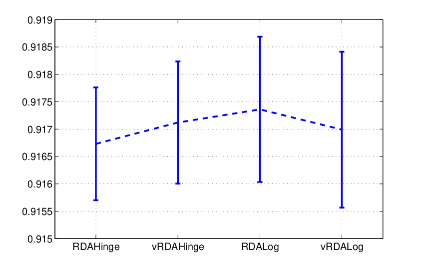
To investigate where the performance gain comes from, we compare the predictions of vRDA by single weight trained at the last sample of each epoch, and the averaged weights learned from all the training samples. In Figure 4, we plot the mean and variance bars with the corrpesonding predictions based on weights trained on 10 epoches. For both Hinge and Log losses, the average predictions have lower variance and better F-Score compared to their single predictions. The large variance for single predictions of Log loss implies that the predictions are quite inconsistent by different epoches samples; thus average predictions is highly desired here.
Conservative Updates
Here, in Figure 5 we compare the performance of RDA and vRDA to illustrate the trade-off by conservative updates with mean and variance bars based on 10 epoches. For Hinge loss, the conservative updates (vRDA) is necessary as the hinge loss is 0 when there is classificaiton mistake; thus vRDA has better F-Score. While for Log loss, RDA is better as even there is a classification mistake, we still has a non-zero loss and need to update the weights accordingly. Another gain by conservative updates is from computational perspective. For vRDA, the frequency ratio of updating weights is amount to the error rate of that of RDA. From our experiments, the training time of vRDA is about 89.7% for Hinge loss and 87.2% for Log loss of RDA. These precentages are not the error rate as there are extra common computaions involved.
7 Conclusion and Discussions
In this paper, we propose a voted RDA (vRDA) method to address online classification problems with explicity regularization. This method updates the predictor only on the subsequence of training examples where a classification error is made. In addition to significantly reducing the computational cost involved in updating the predictor, this allows us to derive a mistake bound that does not depend on the total number of examples. We also introduce the concept of relative strength of regularization, and show how it affects the mistake bound and the generalization performance.
Our analysis on mistake bound is based on the regret analysis of the RDA method [Xia10]. In fact, our notion of relative strength of regularization and error bound analysis also applies to the voted versions of other online algorithms that admit a similar regret analysis, including the forward-backward splitting method in [DS09].
We tested the voted RDA method with -regularization on a large-scale parse reranking task in natural language processing, and obtained state-of-the-art classification performance with fairly sparse models.
References
- [AG07] Galen Andrew and Jianfeng Gao. Scalable training of l1-regularized log-linear models. In Proceedings of the 24th International Conference on Machine learning(ICML 07), pages 33–40, 2007.
- [BB08] Léon Bottou and Olivier Bousquet. The tradeoffs of large scale learning. In J.C. Platt, D. Koller, Y. Singer, and S. Roweis, editors, Advances in Neural Information Processing Systems 20, pages 161–168. MIT Press, Cambridge, MA, 2008.
- [Cha00] Eugene Charniak. A maximum-entropy-inspired parser. In Proceedings of the 1st North American chapter of the Association for Computational Linguistics conference (NAACL 2000), pages 132–139, 2000.
- [CJ05] Eugene Charniak and Mark Johnson. Coarse-to-fine n-best parsing and maxent discriminative reranking. In Proceedings of the 43rd Annual Meeting on Association for Computational Linguistics(ACL 05), pages 173–180, June 2005.
- [Col00] Michael Collins. Discriminative re-ranking for natural language parsing. In Proceedings of the 17th International Conference on Machine learning(ICML), pages 175–182, 2000.
- [Col02] Michael Collins. Discriminative training methods for hidden markov models: theory and experiments with perceptron algorithms. In Proceedings of the ACL-02 conference on Empirical Methods in Natural Language Processing, pages 1–8, 2002.
- [DS09] John Duchi and Yoram Singer. Efficient online and batch learning using forward backward splitting. Journal of Machine Learning Research, 10:2873–2898, 2009.
- [FS99] Yoav Freund and Robert E. Schapire. Large margin classification using the perceptron algorithm. Machine Learning, 37(3):227–296, 1999.
- [FW95] Sally Floyd and Manfred K. Warmuth. Sample compression, learnability, and the vapnik-chervonenkis dimension. Machine Learning, 21(3):269–304, 1995.
- [GAJT07] Jianfeng Gao, Galen Andrew, Mark Johnson, and Kristina Toutanova. A comparative study of parameter estimation methods for statistical natural language processing. In Annual Meeting of the Association for Computational Linguistics (ACL), pages 824–831, 2007.
- [HW95] David P. Helmbold and Manfred K. Warmuth. On weak learning. Journal of Computer and System Sciences, 50:551–573, 1995.
- [LLZ09] John Langford, Lihong Li, and Tong Zhang. Sparse online learning via truncated gradient. Journal of Machine Learning Research, 10:777–801, March 2009.
- [LW12] Sangkyun Lee and Stephen J. Wrigh. Manifold identification in dual averaging for regularized stochastic online learning. Journal of Machine Learning Research, 13:1705–1744, June 2012.
- [MSM93] Mitchell P. Marcus, Beatrice Santorini, and Mary Ann Marcinkiewicz. Building a large annotated corpus of english: The Penn Treebank. Computational Linguistics, 19(2):313–330, 1993.
- [Nes09] Yurii Nesterov. Primal-dual subgradient methods for convex problems. Mathematical Programming, 120:221–259, April 2009.
- [Ros58] Frank Rosenblatt. The perceptron: a probabilistic model for information storage and organization in the brain. Psychological Review, 65:386–407, 1958.
- [SS11] Shai Shalev-Shwartz. Online learning and online convex optimization. Foundations and Trends in Machine Learning, 4(2):107–194, 2011.
- [Xia10] Lin Xiao. Dual averaging methods for regularized stochastic learning and online optimization. Journal of Machine Learning Research, 11:2543–2596, Oct 2010.
- [Zha04] Tong Zhang. Solving large scale linear prediction problems using stochastic gradient descent algorithms. In International Conference on Machine learning (ICML 04), pages 116–123, 2004.
- [Zin03] Martin Zinkevich. Online convex programming and generalized infinitesimal gradient ascent. In International Conference on Machine Learning (ICML03), pages 928–936, 2003.