RUNHETC-2013-20
Ising Spectroscopy II:
Particles and poles at .
A.B. Zamolodchikov1,2
1NHETC, Department of Physics and Astronomy
Rutgers University
Piscataway, NJ 08855-0849, USA
2Institute for Information Transmission Problems
Moscow 127994, Russia
Abstract
I discuss particle content of the Ising field theory (the scaling limit of the Ising model in a magnetic field), in particular the evolution of its mass spectrum under the change of the scaling parameter. I consider both real and pure imaginary magnetic field. Here I address the high-temperature regime, where the spectrum of stable particles is relatively simple (there are from one to three particles, depending on the parameter). My goal is to understand analytic continuations of the masses to the domain of the parameter where they no longer exist as the stable particles. I use the natural tool – the elastic scattering amplitude, with its poles associated with the stable particles, virtual and resonance states in a standard manner. Concentrating attention on the ”real” poles (those corresponding to stable and virtual states) I propose a scenario on how the pattern of the poles evolves from the integrable point to the free particle point , and then, along the pure imaginary , to the Yang-Lee critical point. Waypoints along this evolution path are located using TFFSA data. I also speculate about likely behavior of some of the resonance poles.
October 2013
1 Introduction
This paper is the second part of the project ”Ising Spectroscopy” devoted to detailed study of the particle mass spectrum in the Ising field theory. The latter is the quantum field theory of the scaling domain of 2D Ising model in a magnetic field. It can be defined via the formal action
| (1.1) |
Here represents the unitary conformal field theory with the central charge (which of course is the theory of free massless Majorana fermions), while and are two relevant primary fields of this CFT, with the conformal dimensions and , respectively (see e.g. [1, 2]). In terms of the Ising model, the parameter in (1.1) is suitably scaled magnetic field, while describes the temperature deviation from the Curie point. Away from the critical point the theory (1.1) is massive, and therefore much of its physical content can be understood through its spectrum of particles, stable ones and resonances. Up to overall scale, physical content of the theory (1.1) is controlled by a single dimensionless parameter

| (1.2) |
In particular, the number of stable particles and their masses change with this parameter. Figure 1 shows the behavior of few lowest masses (measured in the units of ) at real . This picture (obtained numerically in [3]) substantiates the scenario originally proposed in Ref. [4]: when changes from to the particle spectrum evolves from a single particle to an infinite tower of ”mesons” formed by weakly confined ”quarks”. In the process, the mass spectrum exhibits rather intricate behavior. Understanding the mass spectrum at intermediate (and not less importantly, complex) values of is the main goal of this project.
In the first part, Ref.[5], the focus was set on the ”low-T” domain , and an attempt was made to understand details of the mass spectrum there in terms of confined ”quarks”. Although many interesting questions about the particle spectrum in that domain (especially the questions regarding how the masses behave near the stability thresholds, and their fate as the resonance states) were left open, here instead we make a foray into the ”high-T” domain . In this region the spectrum of stable particles is actually relatively simple - there is always the lightest stable particle which we denote (and its mass ), and at sufficiently large in addition the heavier particles and appear. The behavior of the masses , and as the functions of is shown in Fig.1. However, it is interesting to understand the analytic continuations of the functions to the region where they no longer represent the masses of stable particles.
Convenient tool for addressing this question is the elastic scattering amplitude . It is a complex analytic function of the rapidity difference of the colliding particles, and its poles in this variable are associated with either stable particles of the theory or virtual or resonance states. In this work I address the question how the pattern of the poles of evolves as changes form to . In fact, the domain of negative real represents only a part of interesting high-T region of parameters where the theory (1.1) is ”real”: at pure imaginary below the so called Yang-Lee critical point [7] the vacuum energy density and the particle mass remain real, and despite the fact that the theory is no longer unitary, it is still meaningful (and interesting) to study its S-matrix. Therefore, I will actually discuss the evolution of the pattern of poles in the wider region, when the parameter changes from to , and then decreases further from to the Yang-Lee point . In this work I will concentrate attention on the ”real” poles of , the ones that correspond to the stable particles and virtual states, because the real poles usually dominate the low-energy behavior of the scattering, and also because they are much easier to analyze. Nonetheless, remarks about some of the resonance poles will be made in Sect.4.
My analysis will be based on general principles, such as positivity of residues of the particle poles in the unitary domain of (1.1), as well as a combination of analytical and numerical data about the mass spectrum of (1.1). The analytical data include exact mass spectra at the integrable points [1, 6, 8], and the results of the perturbation theory expansions around them [9, 11, 12, 14]. Numerical data is obtained by using the Truncated Free Fermion Space Approach (TFFSA) of [3] (which is an adaptation of the TCSA of [15] to the theory (1.1)). In this work I only use the numerical data on the masses of the stable particles, which is extracted from the finite-size energy spectra numerically evaluated via the TFFSA [3]. The numerics is used as a general guidance, and also for estimating numerical values of the parameter (1.2) associated with important waypoints in (1.1). Potentially, TFFSA can be also applied to for numerical evaluations of the scattering phases [16], and masses and width of resonances [17]. This important task goes beyond the scope of this work.
2 S-matrix element. Generalities
Since (1.1) has the particle in its spectrum at all , we find it useful to discuss the other particles in terms of poles in the S-matrix element associated with the elastic scattering. Let us start with brief summary of general analytic properties of this amplitude11 1 The content of this section is mostly an adaptation of the textbook basics of the S-matrix theory (see e.g. [18]) to 1+1 dimensional kinematics. I include it in order to introduce suitable notations.22 2 Although we explicitly speak about the Ising field theory (1.1), the discussion of this section applies to any scattering theory involving a singlet neutral particle ..
2.1 Analyticity and Poles
As usual, it is convenient to characterize the kinematic states of the particles by their rapidities which parameterize the two-momenta as . We will use the notation for the particle with the rapidity . The S-matrix element is defined as
| (2.1) |
where the ”inelastic terms” include all kinematically admissible states of particles , as well as the states with the bound-state particles , , when present in the theory. By standard analyticity, is analytic in the complex -plane, except for poles (which will be of our primary interest here), and branching points associated with the inelastic thresholds. The thresholds are located at the points , where are real positive solutions of the threshold energy equations being the minimal energies of possible combinations of stable particles present in the theory. By introducing the branch cuts from to , and from to , , where , one defines the ”principal sheet” of the Riemann surface associated with 33 3 Certainly, analytic continuation under the inelastic branch cuts, to further sheets of the Riemann surface is possible. At the moment I do not have much to say about analytic properties of the amplitude there.. Henceforth, speaking of complex we always refer to the values at the principal sheet. There, the function satisfies the analytic conditions
| (2.2) |
and
| (2.3) |
The first of them is just the standard expression of the crossing symmetry, while the second follows from elastic unitarity at real with . Eq’s (2.2) and (2.3) imply periodicity , and in what follows we concentrate attention at the strip
| (2.4) |
In view of (2.3) one may limit attention to the ”physical strip” (PS) (which corresponds to the principal sheet of the Riemann surface for the invariant energy square ), but we find it useful to keep view of the full strip (2.4). Since the values of in the strip are determined through its values in the physical strip via (2.3), we will refer to it as the ”mirror strip” (MS).
In addition to the above analytic conditions, satisfies
| (2.5) |
i.e is real analytic function of the variable . It is often useful to distinguish between the positive and negative parts of the physical the mirror strips. These are defined as follows,
| (2.6) |
and
| (2.7) |

The amplitude may have poles on the principal sheet. According to (2.2) and (2.3), it can be generally written as
| (2.8) |
where the product factor accounts for all the poles, so that the ”inelastic phase” is analytic everywhere within the principal sheet of the -surface. It takes the real values in the lacunae of the real -axis, and and hence it is a real analytic function of on the principal sheet. The discontinuity across the inelastic branch cut from to relates to the ”total inelastic cross section” - the total probability of all inelastic processes in the scattering at the center of mass energy - as follows
| (2.9) |
This of course is the 1+1 dimensional version of the optical theorem, which allows one to write down the dispersion relation expressing in terms of . Here I will not discuss the inelastic factor any further. I only note that in integrable theories all inelastic processes are forbidden, the function vanishes identically, and the function reduces to the product factor in Eq.(2.8).
Each factor in the product in (2.8) is responsible for two poles on the principal sheet, located at and , . We denote the residue of at the pole at ,
| (2.10) |
The parameters are subjects to certain general restrictions. Thus, the real analyticity of as the function of demands that are either real or come in complex conjugated pairs; we will refer to the former as the ”real poles” (as opposite to the ”complex poles” with ). The real poles will be of the central interest in our discussion below. The residues at the real poles are real, and we will call the the real pole ”positive” if , or ”negative” if . As follows from (2.2), if the pole at is positive, the associated pole at is negative, and vice versa. For the complex poles we call the pole at conjugated to the pole at .
Real poles located in the PS are generally interpreted in terms of the stable particles of the theory - the bound states. In unitary field theories the positivity requires that any positive pole with is identified with the s-channel bound state with the mass
| (2.11) |
while the associated negative pole at represents the same particle in the u-channel. In a non-unitary theory the s-channel bound state may be represented by a negative pole (we will encounter this situation in the theory (1.1) at pure imaginary magnetic field ). Real poles located in the mirror strip do not correspond to any stable particles; borrowing terminology from the potential scattering, such poles are referred to as the virtual states.
The (non)symmetry of the action (1.1) generally allows the particle to appear as the bound state pole in the scattering. This ” property” means that the product in (2.8) always 44 4 At special values of the parameters in (1.1) this pole factor can be canceled by another factor in the product; we will see that this happens only at . involves the factor with
| (2.12) |
This factor produces two poles in the PS; one at , interpreted as the s-channel pole associated with the particle , and another at , which is the corresponding u-channel pole.
Complex poles in the physical strip are forbidden by causuality. The complex poles in the MS are generally interpreted as the resonance states. Because of the crossing relation (2.2), which can be equivalently written as , the pattern of the resonance poles in the MS is symmetric with respect to the inversion ( rotation) around the point in the plane. For this reason the resonance content of the elastic scattering is completely determined by the poles located in MS(+), Eq.(2.7). For a resonance pole at
| (2.13) |
with real and the s-channel complex mass is
| (2.14) |
so that both and are positive, and such poles admit interpretation as the resonance states in the s-channel, with and identified with the center of mass mean energy and the width of the resonance state55 5 Of course, only if it is fair to associate the pole at with a metastable state with a long lifetime and well defined energy. However, for the luck of better term, we refer to all the complex poles in MS(+) as the s-channel resonances.. Complex poles located in are interpreted as the u-channel resonances.
Because of the crossing symmetry (2.2) of the scattering, the resonance poles generally appear in the MS(+) in pairs: comes along with . We call these pairs ”cross-conjugated”66 6 Cross-conjugated points are complex conjugated in terms of the variable . In fact, it is easy to see that as the consequence of and (2.2) the amplitude is real analytic function of .. Exceptions are the poles with ; for such poles . We call such special poles self cross-conjugated (not to be confused with real poles defined above).
3 Pole evolution
Let us return to the specific field theory (1.1). In this work we concentrate attention at the high-T domain , where the theory has an unbroken symmetry . As the result, at the most important characteristics (mass spectrum, S-matrix) are even functions of . Therefore in this domain it is convenient to consider the dependence of the theory on the dimensionless variable
| (3.1) |
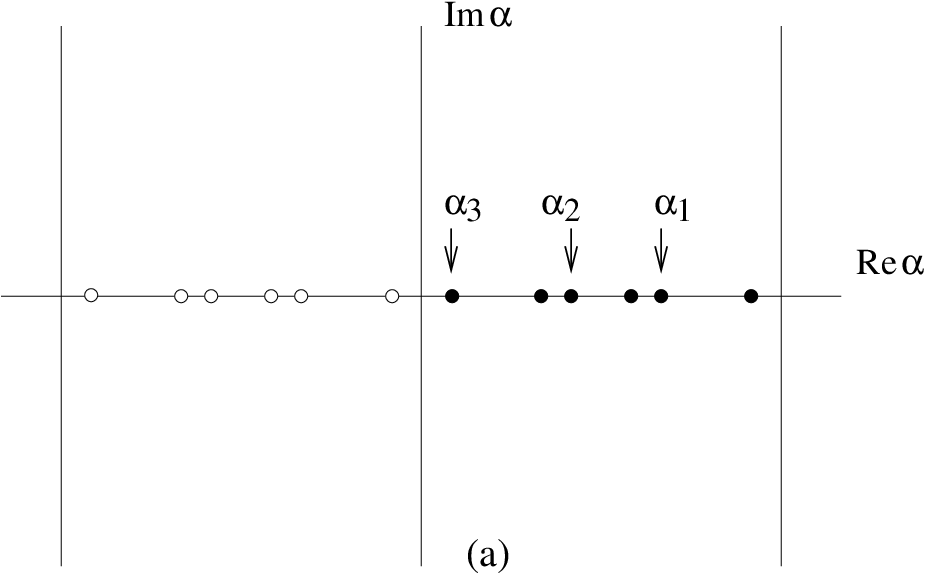
It is commonly assumed that, as the functions of this variable, the characteristics of the theory admit analytic continuation to the whole complex -plane with the branch cut along the negative real axis, from to , as shown in Fig.3a. The numerical value
| (3.2) |


was estimates in [3]77 7 The estimate in (3.2) is slightly better then the one given in [3]; it was obtained by detailed numerical analysis of the mass near the Yang-Lee critical point [19].. The point is the so called Yang-Lee edge singularity. It is a critical point in the sense that the mass of the particle vanishes at this point (see Fig.3b) [7]. The CFT associated with this critical point was identified as the nonunitary minimal model with the central charge [20].
At real positive the theory (1.1) is unitary (both the parameters and can be taken real). The negative part of the real axis in Fig.3a is realized by pure imaginary values of the magnetic field , so here the unitarity is violated. However, at real the theory remains ”real” in the sense that the ground state energy and the particle mass remains real, and the S-matrix still enjoys all the real analyticity (but not positivity) conditions stated in Sect.2 88 8 At these properties are lost. The ground state becomes two-fold degenerate, with the complex conjugate values of the associated vacuum energies. The particle masses become complex as well, and all reality conditions of the S-matrix described in Sect.2 are violated. We do not discuss this interesting regime here.. The most obvious manifestation of the non-unitarity in this domain is negative residue of the -particle pole of (see below).
In this work we discuss the theory (1.1) at the values of the parameter along the segment of the real axis in the Fig.3a. The spectrum of stable particles is relatively simple - there is the particle at all these values of , and at sufficiently large positive (at , and at , respectively, where , ) the stable particles and appear in the spectrum 99 9 Also, at , which corresponds to one of the integrable points (see below), five additional particles appear; at they become resonance states, as we briefly discuss in Sect.4. However, the spectrum of the virtual and resonance states is more rich. Below I describe the evolution of the pole structure of as the parameter changes from to , and then from to the Yang-Lee point . I will pay most attention to the real poles; once a pole at leaves the imaginary -axis, I usually will not attempt to follow its fate as a complex pole. The reasons for this are as follows. First, the low-energy behavior of the the elastic scattering amplitude is usually dominated by its real-pole content. But more significantly, there still is very little amount of data, both analytical and numeric, about high-energy behavior of scattering amplitudes (see however [14]), and about high energy resonance states in particular. The main goal of this note is to put forward a scenario for the evolution of the real poles of when changes from down to . However, I will make remarks about evolution of some resonance poles in Sect.4.
Although the parameter is quite suitable for the needs of the present discussion, to facilitate comparison with Refs.[3, 5] I will frequently discuss simultaneously in terms of the related scaling parameter defined in Eq.(1.2). Generally, these parameters are related by the complex-analytic map
| (3.3) |
with the branch chosen in such a way that the negative part of the -axis is mapped to real positive . Then, while positive real are represented by negative real , negative correspond to complex along certain rays in the -plane,
| (3.4) |
The segment is given by , where
| (3.5) |
3.1 Integrable points
There are three special points in the parameter space of the theory (1.1) where the amplitude is known exactly:
(a): (), which corresponds to , . At this point the theory (1.1) is integrable, and its spectrum involves 8 stable particles whose masses are given by the components of the Perron-Frobenius vector of the Cartan matrix of the Lie algebra . The scattering theory is described by the reflection-less factorizable S-matrix [6]. is the lightest particle, and elastic scattering is given by (2.8) with and three pole factors,
| (3.6) |
All the poles here are located in the physical strip, at and , , where
| (3.7) |
While the pole at represents the s-channel particle itself, the poles at and correspond to heavier stable particles and , with the masses
| (3.8) |
As usual, the poles at are the u-channel manifestations of the same particles. The pattern of poles and zeroes of is shown in Fig.4a. Although the poles associated with the higher stable particles are not present in , such poles show up in other elastic scattering amplitudes [6]. Observe that (i) has no zeros in the PS, and (ii) There is one u-channel pole in between any two s-channel poles . These two conditions, together with easily verified , guarantee that the residues at the s-channel poles , , are all positive.
(b): (), which corresponds to with . At zero magnetic field the (1.1) reduces to the theory of free Majorana fermi field with the mass . The free particle is , hence at this point , and
| (3.9) |
(c): (). The integrable theory appears in the scaling limit near the Yang-Lee critical point. As was already mentioned, as approaches the Yang-Lee point the mass of the particle vanishes as
| (3.10) |
while the masses of all resonances (there are no other stable particles near the Yang-Lee point) remain finite in this limit. Therefore, when measured in the units of , all these masses depart to infinity at . The resulting scattering theory of the particles turns out to be integrable, with the S-matrix given by [8]
| (3.11) |
Except for the poles at , Eq.(2.12), and , which correspond to the s- and u- channel manifestations of the , there are no real or complex poles. Note that , and that is negative.
3.2 Positive (real negative )
The goal of this subsection is to analyze how the pattern of poles in (3.6) (see Fig.4a) evolves into the trivial pattern (no poles, no zeros) associated with the free particle S-matrix (3.9) when changes from down to . The arguments will be based partly on the general properties of the S-matrix (see Sect.2), and partly on the numerical and perturbative data about the mass spectrum of (1.1). Since the theory (1.1) with real and is unitary, the general properties include the condition that all s-channel poles associated with stable particles remain positive during the evolution. We also assume that the parameters
| (3.12) |
depend on in an analytic way along the whole segment 1010 10 Generally, there are no good reasons to expect themselves to be analytic in the whole range of the coupling parameter. Rather, one should expect analyticity of the coefficients of the polynomial , while are allowed to have algebraic singularities. We will see below that this subtlety is irrelevant in the simple scenario suggested below.. The pole at is interpreted as the s-channel particle , and therefore remains fixed to the value (2.12) during the whole evolution. We need to figure out the behavior of the remaining .
When is large (equivalently, is small) the theory (1.1) is in the perturbative domain around the integrable point (a). The leading corrections to the mass ratios and were found in [9, 12], using the form factor perturbation theory. From these, and the numerical data, one finds
| (3.13) |
| (3.14) | |||
| (3.15) |
When decreases from to negative values, the parameters and both decrease, so that the associated poles move towards zero (see Fig.4b). Simultaneously, a number of additional complex poles appear; these resonance poles are ignored in Fig’s 4 and 5. I postpone comments about them to Sect.4. At certain value the pole at crosses zero. At this point . Numerical data yields
| (3.16) |


and
| (3.17) |
At the pole leaves the PS and enters the MS (Fig.4c), so that the particle disappears from the spectrum of stable particles, becoming a virtual state. After crossing to MS becomes a negative pole (the residue ). However, we will still associate the pole at with the ”particle” , now a virtual state, and call it the ” pole”. Note that although below the number of stable particles in (1.1) changes from three to two, the number of pairs of real poles in remains equal to three all the way down to somewhat lower value of (see Eq.(3.21) below).
When continues to decrease from down, the next interesting event occurs at
| (3.18) |
where the mass ratio reaches the value . At this point the pole at , on its way towards zero, crosses the point where the u-channel pole of the particle sits. After that, these poles interchange their order along the imaginary -axis. Without additional poles or zeros around, after such ”pole crossing” the formerly positive pole would become a negative one, while the pole at would become a positive pole. But unitarity demands that the poles must retain their signatures as long as remains real. The only way this can happen is if there is a zero of located in the PS which passes through at the same point . There is only one pair of zeros in the PS in this domain of - the zeros at and (these are the ”mirror images” of the poles and which at are already in the MS). Therefore, we must have
| (3.19) |
The pattern of poles at immediately above and immediately below are shown in Fig.4c and Fig.4d.
As decreases further from , already negative continues to decrease, and at certain it crosses . At this point the poles and collide at the middle of MS,
| (3.20) |


and at they become a pair of self cross-conjugated complex poles, moving away from the imaginary -axis as with real (Fig.5a). Therefore, below the number of real poles changes from three to two. Note that at the analytic continuation of takes the value , and immediately below this point becomes complex. The numerical value
| (3.21) |
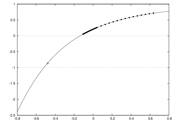
was estimated by extrapolating the data for from the domain of above , where the mass ratio is directly available from TFFSA. The plot in Fig.6 suggests that as decreases further down from the poles and rapidly move away from the real axis, so that almost immediately below the pole becomes a high energy resonance. At the moment we do not have anything but speculations about its fate at substantially below 1111 11 Simple form (3.9) suggests that this pair of poles must depart to infinity either at or at some intermediate value between and . The result of Ref.[14] seems to rule out the first possibility..
As for the remaining real poles, at below the pole continues to move towards zero, and at it too crosses into MP. Again, from TFFSA data on we have
| (3.22) |
Below the particle ceases to exist as a stable particle, becoming a virtual state instead, but as with , we will continue to call the ” pole”. At the real spectrum of stable particles of (1.1) involves a single neutral particle . The patterns of poles and zeros of just above and just below are shown in Figures 5b and 5c, respectively. Note that since below the pole remains real, the analytic continuation of remains real and below as well; in fact, it is real for all (see below).
As decreases further, the pole sinks deeper into MS, and eventually it approaches the point where the fixed zero (mirror image of the u-channel pole ) sits. When is close to the residue at the pole becomes small (recall that in this limit the mirror zero of the u-cannel pole approaches the pole, as seen in Fig.5d),
| (3.23) |
This is exactly what is expected in (1.1) at small . Indeed, the residue vanishes at since we have to have (3.9), and the leading perturbative contribution is [14]
| (3.24) |
where is the constant appearing in the one-particle matrix element [21]. We conclude that at large negative approaches from above as
| (3.25) |
In the limit (i.e. at ) the pole gets canceled by the fixed zero at , and thus all real poles disappear, consistently with (3.9). Of course, (3.9) also demands that all the resonance poles (which we left without attention so far) disappear in this limit as well.
3.3 Negative
In the previous subsection we have described the evolution of the real poles of when changed from to (equivalently, real changed from to ). This evolution can be extended to negative above the Yang-Lee point . The latter values correspond to pure imaginary between zero and . In terms of we will be dealing with the values along the rays (3.4) with .
As we have seen above, at small positive the pole is located close to the right of the fixed zero , and at this zero exactly cancels the pole, leading to the trivial amplitude (3.9). As becomes small negative the pole re-emerges to the left of the fixed zero . In terms of the variable defined in Eq.(3.4) we have
| (3.26) |


Correspondingly, at small negative the zero appears close to the right from the pole (Fig.7a). The equation (3.24) remains valid at negative ; the fact that the residue at the pole becomes negative is consistent with the non-unitarity of the theory at .
As continues to decrease further from zero, the parameter , already negative at , continues to decrease as well, and at certain value it crosses the value . Although below , and hence , can not be extracted directly from the TFFSA data, it can be estimated using certain dispersion relation [19]. This yields the numerical value of , which we quote in terms of the variable (Eq.(3.4)) as well as ,
| (3.27) |
At the poles and collide at , and at they move away from the imaginary -axis as a pair of self cross-conjugated complex poles. The patterns of real poles of slightly above and slightly below are shown in Figs 7b and 7c, respectively. Finally, as approaches from above, the poles depart to infinity1212 12 It is possible that additional resonance poles exist in this domain. In any case, as approaches , by scaling arguments all the resonance poles are expected to move to infinity as ., and the only poles of left are the s- and u- channel poles at and (Fig.7d). Simultaneously, as the discontinuities across the inelastic branch cuts disappear1313 13 The discontinuities across the inelastic branch cuts go down as fast as , as we argue in [19]., and in the limit reduces to (3.11).
4 Resonances
Although in this work I am not going to discuss behavior of the resonance poles in any systematic way, here some comments on this issue will be made.
Clearly, the amplitude generally has some number of resonance poles. We have already observed that the and poles at and , together with their cross-poles, become self cross-conjugated complex poles when gets below certain values and , respectively. But certainly there may be more resonance poles. For instance, it was already mentioned that the integrable theory at involves eight stable particles which we refer to as , , …, . Only the first three of these particles, , and , remain stable when is shifted away from the integrable point . The other five particles loose stability becoming resonances, and their masses acquire imaginary parts, as in (2.14). In fact, for the lowest of them, and the widths and were computed to the order via form-factor perturbation theory in [11]. Below I attempt to follow the fate of some of the associated complex poles at negative , until the poles leave the principal sheet of the Riemann surface of .
Let me start with the following (well known) observation. At the mass of appears to be located very close below the threshold , i.e. the difference
| (4.1) |
is numerically small in the units of . This means that at the particle can be interpreted as a weakly coupled two-particle bound state. It is also well known that in dimensions neutral particles that form two-particle bound state also tend to form three- four- and generally -particle bound states, with the binding energies
| (4.2) |
where is the binding energy of the two-particle bound state. This is because when the particles are weakly bound, the system is well approximated by non-relativistic Bose particles with attractive delta-function interaction, from which (4.2) follows [22, 23]. Indeed, typical momenta of the particles constituting a weakly coupled bound state are small in the units of , making it possible to use non-relativistic theory. Also, the size of the bound state is much greater then the effective interaction range (), allowing to approximate the pairwise interactions by delta-function potentials. One can show that direct multi-particle interactions become negligible in the limit when the binding energy goes to zero. Note that even if is small, this approximation applies only to finitely many lowest -particle bound states since at sufficiently large the energies (4.2) become comparable with , and the approximation breaks down.
The above argument suggests, in particular, that at we have to observe weakly coupled three- , four- , and perhaps multi - particle bound states of , with the binding energies approximately given by (4.2). And indeed, as it turns, is numerically close to , is close to , and is close to . Using exact mass ratios [6], let us compute the binding energies and compare them to the approximation (4.2),
| (4.3) | |||
I would like to emphasize that at , while the mass spectrum of [6] is exact, (4.2) is only an approximation – after all, in (4.1) is only numerically small. Nonetheless, numerical agreement between the exact mass spectrum and the weak binding approximation (4.2) is remarkably good - curiously enough, the Perron-Frobenius vector of the Cartan matrix of ”knows” about weakly interacting particles. Also note that in (4.3) is already comparable to , so for greater values of one should not expect the above arguments to be too reliable.
Consider small nonzero . Now the integrability of the theory (1.1) is broken, and the particles , , …, become unstable against decays into the lighter particles. Correspondingly, the masses immediately become complex, with small imaginary parts . Although all five particles , , …, turn into resonances, below we argue that the widths of the resonances , , remain small at all between and , and go back to zero as approaches . When decreases below these three particles likely cease to exist even as the resonance states (the corresponding poles leave the principal sheet of the Riemann surface of ). It is plausible that in a similar manner, the widths of the resonances and go to zero when approaches from above, and below these resonances disappear.
As was already discussed in Sect.3, as becomes negative, the parameter , already as small as at , moves even closer to zero. As long as it remains positive, the particle remains stable, but its mass approaches , and its description as the weakly coupled bound state of two particles with the binding energy
| (4.4) |
become yet more accurate. Therefore there is even better reason to expect the presence of weakly coupled -particle bound states with greater then 2 when gets closer to . Moreover, Eq.(4.2) gives the better approximations of the binding energies the closer to zero is. Of course, at nonzero exact integrability is violated, and the bound states with are unstable against decays into lighter particles. However, it is possible to argue that the decay rates of the -particle bound states are suppressed at least as , therefore these resonances become very narrow () as approaches from above. When crosses the resonance poles merge with inelastic thresholds, and then likely move on to further sheets of the Riemann surface of . Below the particles , , disappear even as the resonance states, at least in the definition given in Sect. 2. On the basis of the above argument I predict that the width of the resonances , , remain very small in the domain , and their masses in this domain are very well approximated by the equation , . It would be interesting to test this prediction against numerical data. Existing TFFSA data is consistent with the prediction, but substantial improvements (mostly in proper handling of the finite size effects) are needed in order to make meaningful comparison.
There are several questions related to the above argument. If the binding energy is sufficiently small, one expects to have -particle bound states with any . But at we do not see bound states with . Perhaps at this point the binding energy is not sufficiently small. However as decreases, and the binding energy becomes smaller, the higher bound states have to appear. Where they could come from? At this time I do not have good answer to this question. I could only speculate that their emergence can interfere with the formations of bound states of heavier resonances. Note in this connection that if the weak binding approximation (4.2) with is applied at , the resulting binding energy would be numerically close to the difference .
Another question concerns the fate of the resonances and , which were missed in the above scenario. Their masses [6]
| (4.5) |
do not seem to suggest any weakly coupled bound state structure. At small , of course they too become resonances. Then, apart from the opening of narrow decay channel(s), there are no reasons to expect dramatic structural changes in these particles at small nonzero . And indeed, TFFSA data show the presence of the and (somewhat less convincingly) resonances at well below . However the ratios and ( are the real parts of the masses , Eq.(2.14)) increase as decreases from . Recall that as approaches (Eq.(3.22)) from above, the mass gets close to the threshold – now becomes weakly coupled bound state. Therefore, at slightly above one expects to have a number of narrow resonances with the (complex) masses close to , , and with the ”binding energies” well approximated by (4.2), where now . It is tempting to speculate that as decreases to the values slightly above , the resonances and assume the role of the weakly coupled three- and four- particle bound states of . This would suggest that at these values of the imaginary parts become small, while the real parts and appear closely below and , respectively. Again, the existing TFFSA data seems to be consistent with this scenario, although more detailed analysis is desirable.
Acknowledgments
I would like to thank Sergei Lukyanov, Alexei Tsvelik, and especially Barry McCoy for many invaluable discussions and interest. I gratefully acknowledge hospitality of the Simons Center for Geometry and Physics where parts of this work were done.
The research is supported in part by DOE grant DE-FG02-96ER40959.
References
- [1] C. Itzykson, J.-M. Drouffe, Statistical Field Theory, Cambridge University Press, 1989.
- [2] P. Di Francesco, P. Mathieu, D. Sénéchal, Conformal Field Theory, Springer, 1996
- [3] P. Fonseca, A. Zamolodchikov, Ising field theory in a magnetic field: Analytic properties of the free energy, J. Stat. Phys. 110, (2003) 527-590; hep-th/0112167
- [4] B.M.McCoy, T.T.Wu, Two-dimensionsl Ising field theory in a magnetic field: breakup of the cut in the two-point function, Phys. Rev. D18 (1978) 1259-1267.
- [5] P. Fonseca, A. Zamolodchikov, Ising spectroscopy. I. Mesons at , RUNHETC-2006-13, Dec 2006. 44pp; hep-th/0612304
- [6] A. Zamolodchikov, Integrals of Motion and S Matrix of the (Scaled) T=T(c) Ising Model with Magnetic Field, Int. J. Mod. Phys. A4 (1989) 4235; Integrable field theory from conformal field theory, Adv. Stud. Pure Math. 19 (1989) 641-674
- [7] M.E. Fisher, Yang-Lee edge singularity and field theory, Phys. Rev. Lett. 40 (1978) 1610-1613.
- [8] J. Cardy, G. Mussardo, S Matrix of the Yang-Lee Edge Singularity in Two-Dimensions Phys. Lett. B225 (1989) 275
- [9] G. Delfino, G. Mussardo, P. Simonetti, Nonintegrable quantum field theories as perturbations of certain integrable models, Nucl. Phys. B473 (1996), 496-508; hep-th/9603011.
- [10] P.Fonseca, A.Zamolodchikov, Ward identities and integrable differential equations in the Ising field theory, RUNHETC-2003-28, Sep 2003; hep-th/0309228
- [11] G. Delfino, P. Grinza, G. Mussardo Decay of particles above threshold in the Ising field theory with magnetic field, Nucl. Phys. B737 (2006) 291-303; hep-th/0507133
- [12] G. Delfino, Integrable field theory and critical phenomena: The Ising model in a magnetic field, J.Phys. A37 (2004) R45; hep-th/0312119
- [13] [8] G. Delfino, ”Integrable field theory and critical phenomena: The Ising model in a magnetic field”, J. Phys. A 37 (2004) R45, hep-th/0312119
- [14] A. Zamolodchikov, I. Ziyatdinov, Inelastic scattering and elastic amplitude in Ising field theory in a weak magnetic field at : Perturbative analysis, Nucl. Phys. B849 (2011) 654-674; arXiv:1102.0767 [hep-th]
- [15] V.P. Yurov, Al.B. Zamolodchikov, Truncated Conformal Space Approach To Scaling Lee-Yang Model, Int. J. Mod. Phys. A5 (1990) 3221-3246.
- [16] V.P. Yurov, Al.B. Zamolodchikov, Truncated fermionic space approach to critical 2D Ising model with magnetic field, Int. J. Mod. Phys. A6 (1991) 464-485
- [17] B. Pozsgay, G. Takacs, Characterization of resonances using finite size effects, Nucl. Phys. B748 (2006) 485-523; hep-th/0604022
- [18] R.J. Eden, P.V. Landshoff, D.I. Olive and J.C. Polkinghorne, The Analytic S-Matrix, Cambridge U. Press, 1966.
- [19] A.Zamolodchikov, Ising field theory in a magnetic field: Yang-Lee singularity, in preparation.
- [20] J. Cardy, Conformal Invariance and Yang-Lee Edge Singularity in Two Dimensions, Phys. Rev. Lett. 54 (1985) 1354-1356.
- [21] T.T. Wu, B.M. McCoy, C.A. Tracy and E. Barouch, Spin-spin correlation functions for the two-dimensional Ising model - exact theory in the scaling region, Phys. Rev. B 13 (1976) 316-374
- [22] F.A. Berezin, G.P. Pochil, V.M. Finkelberg, Moscow Univ. Vestnik 1, 21 (1964); J.B. McGuire, J. Math. Phys. 5 (1964) 622; E. Brezin, J. Zinn-Justin, C. R. Acad. Sci. (Paris) B263 (1966) 670; C.N. Yang, Phys. Rev. Lett. 19 (1967) 1312 and Phys. Rev. 168 (1968) 1920
- [23] F. Calogero, A. Degasperis, Comparison between the exact and Hartree solutions of a one-dimensional many-body problem, Phys. Rev. A 11 (1975) 265-269