Beauty is more attractive: Particle Production and Moduli trapping with Higher Dimensional Interaction
abSeishi Enomoto**
*
e-mail: enomoto@eken.phys.nagoya-u.ac.jp,
cSatoshi Iida††
†
e-mail: saiida@th.phys.nagoya-u.ac.jp,
acNobuhiro Maekawa‡‡
‡
e-mail: maekawa@eken.phys.nagoya-u.ac.jp,
dTomohiro Matsuda§§
§
e-mail: matsuda@sit.ac.jp
a Kobayashi Maskawa Institute, Nagoya University, Nagoya 464-8602, Japan
b Institute of Theoretical Physics, Faculty of Physics, University of Warsaw, Hoa 69, 00-681 Warsaw, Poland
c Department of Physics, Nagoya University, Nagoya 464-8602, Japan
d Laboratory of Physics, Saitama Institute of Technology, Saitama 369-0293, Japan
We study quantum effects on moduli dynamics arising from particle production near the enhanced symmetry point (ESP). We focus on non-renormalizable couplings between the moduli field and the field that becomes light at the ESP. Considering higher dimensional interaction, we find that particle production is significant in a large area, which is even larger than the area that is expected from a renormalizable interaction. It is possible to find this possibility from a trivial adiabatic condition; however the quantitative estimation of particle production and trapping of the field in motion are far from trivial. In this paper we study particle production and trapping in detail, using both the analytical and numerical calculations, to find a clear and intuitive result that supports trapping in a vast variety of theories. Our study shows that trapping driven by a non-renormalizable interaction is possible. This possibility has not been considered in previous works. Some phenomenological models of particle physics will be mentioned to complement discussion.
1 Introduction
Supersymmetric (SUSY) models are one of the most promising candidates of the theory beyond the standard model (SM). One of the characteristic features of the SUSY models is that they have a number of light scalar fields called flat directions or moduli, which describes deformations of the effective system. Therefore, these models may have many quasi-degenerated vacua, which could be stable or metastable. Our Universe may arise from one of those vacua. Since the vacuum expectation value (VEV) of the moduli determines the low-energy effective theory, it is important to find the way how these moduli find their vacuum when the moduli are not static. Thinking about the very early stage of the cosmological evolution, these fields might have a large kinetic energy compared to their potential energy.
A decade ago, Kofman et.al. suggested in their paper “Beauty is attractive” [1] that a vacuum could be chosen because it is attractive. Their critical observation is that since new degrees of freedom become light when the modulus passes through the enhanced symmetry point (ESP), these species could be produced by the quantum effects and could alter the dynamics in such a way as to drive the moduli towards the ESP. They called this mechanism “trapping”. Their basic argument was based on the effective theory that contains an interaction between two scalar fields:
| (1.1) |
The interaction may arise in a system of moving branes, in which a gauge symmetry of the effective action could be enhanced when branes pass through.
On the other hand, we know that in some cases moduli in the effective action may not be coupled to light fields through renormalizable couplings, in the sense that they may have interactions suppressed by the cutoff scale. A typical example could be the neutrino mass in the see-saw mechanism, which couples to the Higgs scalar field through higher dimensional interaction in the low energy effective theory.11 1 Of course the Higgs is not a moduli field. We think there is no confusion in this analogy. Note that in this paper we are considering a more general situation, which has not been considered in Ref. [1]. We are extending the original scenario to include higher dimensional interaction, to show that such interaction is indeed responsible for particle production and trapping. We consider interaction:
| (1.2) |
which is sometimes called “higher dimensional” interaction, since the mass dimension of is higher than four.22 2 Alternatively, particle creation and dissipation could be caused by the Kaluza-Klein tower of the extra dimensions [2]. More recently, “higher dimensional field space” has been considered in Ref. [3, 4]. We hope there is no confusion in those “higher dimensional” arguments.
One might think that higher dimensional interaction is not important because it is suppressed by the cutoff scale; however a trivial adiabatic condition (, which will be defined later in this paper) suggests that particle production is possible in a wider area than conventional trapping. Although the qualitative argument based on the adiabatic condition is suggesting that higher dimensional interaction could be important, it is not quite obvious whether such interaction is responsible for trapping. Obviously, the quantitative estimation of quantum particle production is far from trivial.
In this paper, we study the production of the particles when higher dimensional interaction is responsible for the mechanism. The amount of particle production will be calculated extending the method developed in Ref. [5]. Our conclusion is that particle production via higher dimensional interaction is significant in a wide area around the ESP. Our result is consistent with the naive estimation based on the adiabatic condition. Moreover, using the numerical calculation, we demonstrate thattrapping is indeed possible via higher dimensional interaction. Interestingly, as is expected from the adiabatic condition, we confirmed that the area of trapping becomes wider than conventional trapping.
Our conclusion is that the mechanism can play an important role in selecting the vacuum in the early Universe. Note that even if one is considering the conventional ESP, one might have to consider higher dimensional interaction, since in reality there could be multiple fields that are responsible for the symmetry breaking. In that case quantum particle production must be calculated when the original symmetry is already broken by the other fields (but higher dimensional interaction could remain).33 3 We need a field whose mass is determined by higher dimensional interaction. Note that could not be identical to the conventional , which becomes massive when the gauge symmetry is broken. See Sec.5.1 for more details, in which we consider a toy model. Particle production in the multi-field dynamics is rather complicated. This possibility has never been considered before. We found that trapping is indeed possible for such ESPs, where the gauge symmetry could not be recovered but higher dimensional interaction may arise.
2 Basic mechanism of quantum particle production and trapping at an ESP
First we review the basics of particle production and trapping of Ref. [1]. Consider the Lagrangian:
| (2.1) |
which consists of two scalar fields (complex) and (real). Here, is a field in classical motion, while is the field that is produced by the quantum effect. For simplicity, we assume that is homogeneous in space, so that we can write .
When and the back-reaction is negligible, the equation of motion gives
| (2.2) |
where is the velocity of , and is called the impact parameter. This solution is valid as far as the adiabatic condition () is satisfied for . Here, we defined
| (2.3) |
where is the momentum of . For a low momentum mode () and a small impact parameter (), the adiabatic condition leads to
| (2.4) |
Consider the trajectory shown in Figure 1, in which comes into the “non-adiabatic” area , where the adiabatic condition is violated and the quantum back-reaction is not negligible.

The observation in Ref. [1] is that in that area the mass of becomes light and the kinetic energy of can be translated into -particle production. The number density of the field has been evaluated as
| (2.5) |
This result shows that particle production is indeed significant in the area . The result is consistent with the naive estimation from the adiabatic condition.
After the quantum excitation of , moves away from the ESP. However, the interaction causes back-reaction, since the motion increases the mass of particle (). As a result, the energy density of increases as moves away from the ESP. One will find
| (2.6) |
The energy density changes the potential of . The induced potential is a linear potential measuring the distance from the ESP. See also Fig. 2.
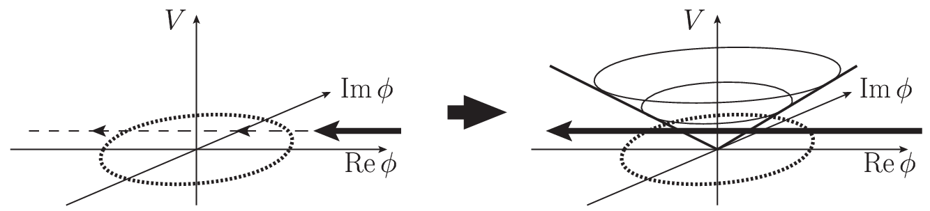
After that, goes up the potential until the initial kinetic energy is comparable to the potential energy, where makes a turn and goes back to the ESP again. Then, there will be another production of , giving additional back-reaction. Finally, is “trapped” around the ESP. Numerical calculation of the trajectory is shown in Figure 3.

3 Analytical calculation with higher dimensional interaction
In the previous section we reviewed quantum particle production when passes through the non-adiabatic area around the ESP. Trapping has already been confirmed [1] for a renormalizable interaction given in Eq.(2.1). In this section, we consider higher dimensional interaction instead of renormalizable one. We start with the Lagrangian:
| (3.1) |
where reproduces a renormalizable interaction. One can check the consistency of our calculation for .
First consider the non-adiabatic condition. From , we obtain
| (3.2) |
where and are considered. The above (naive) condition shows that the area may become even larger for larger . A similar speculation could arise from the effective mass near the ESP, which is given by
| (3.3) |
One can see that is lighter for larger . Since the kinematically allowed mass () is bounded from above by the initial kinetic energy of , we can expect that the area of particle production could be wider for larger . On the other hand, the interaction seems to be weaker for larger . Therefore, there could be a tension between these effects, which cannot be solved without looking into more details of the mechanism.
3.1 Equations and trajectory without particle production
Before solving Eq.(3.1), we need to include for the normalization:
| (3.4) |
where is defined by
| (3.5) |
and is a frequency of the quantum field defined by
| (3.6) |
is needed to subtract a divergence in the Coleman-Weinberg potential. Note that we are considering the effective action that has an explicit cutoff scale.
Next, we define the wave function for . Then the creation/annihilation operators are defined as
| (3.7) |
where satisfy the commutation relations
| (3.8) |
and satisfies the norm condition
| (3.9) |
We obtain the equations of motion:
| (3.10) |
| (3.11) |
Here, we assumed that is homogeneous in space. Since is the homogeneous function of , the wave function is also homogeneous in space.
Let us examine the initial conditions. For , we can define initial quantities and at . Using the WKB approximation for , we consider the initial wave function
| (3.12) |
This WKB solution is valid as far as the adiabatic condition is satisfied:
| (3.13) |
Substituting (3.12) into (3.10), we obtain the trivial solution
| (3.14) |
which reproduces the classical motion (2.2). The above solution is valid when quantum production and the back-reaction are negligible.
3.2 Quantum particle production and the back-reaction
As approaches toward the ESP, the adiabatic condition (3.13) will be violated. In that case the WKB approximation (3.12) is no longer valid. We consider [5, 6]
| (3.15) |
The equation of motion (3.11) gives
| (3.16) | |||||
| (3.17) |
where the initial conditions are and . We can evaluate the number density of the light field from , using the relation
| (3.18) |
Considering as the 0-th order approximation, one can find the exact solution when . (See the review in Sec.2.) The situation changes when , since we do not have the obvious solution that can be used for . Therefore, we need another calculational method that is valid for higher dimensional interaction. An obvious way is to find using the numerical calculation, which will be demonstrated later in this paper. The numerical calculation supports our analytical calculation.
Because of the complexity of the method, the details of the analytical calculation will be described in Appendix A. We obtained
| (3.19) |
where and are numerical coefficients. (See Table 1.)
This formula is valid for the impact parameter
| (3.20) |
Considering , one can easily check that Eq.(3.19) is consistent with Eq.(2.5). Note that the leading order (the first term in eq. (3.19)) is independent of the impact parameter . (Note however that the condition (3.20) is crucial.) Moreover, if we consider a large- limit, the area of particle production becomes larger. Significantly, the area of quantum particle production can become larger than the conventional scenario, although the number density () has a suppression factor when . The above result is consistent with the naive argument based on the adiabatic condition. Of course, we need to examine the back-reaction from particle production in more detail; otherwise trapping is not obvious.
The back-reaction is caused by the effective potential generated by the energy density :
| (3.21) |
Note that the Hamiltonian gives
| (3.22) |
where is the VEV of the Hamiltonian . Here, we can see that trapping force is weak near the ESP, but it becomes stronger when is away from the ESP. Except for a low-velocity limit (), trapping force is significant when approaches .
In the next section, we will examine the trapping mechanism using the numerical calculation.
4 Numerical results
In this section we present our numerical calculation and compare it with the analytical estimation, so that one can easily examine the consistency between them. Then, we can examine the trapping mechanism using the trajectory .
Our numerical results are obtained by solving the equations of motion (3.10) and (3.11). The initial condition is defined using the WKB approximation, since is initially away from the non-adiabatic area. In this paper we consider , where the initial velocity is considered for and . For , we take , where is obtained by taking the differential of Eq.(3.12), which gives
| (4.1) |
4.1 Number density after quantum particle production
The number density after quantum particle production is obtained from and [7]:
| (4.2) |
We show our results for and in Figure 4. Considering the initial energy density (for and ), we can examine the ratio of the induced potential energy at to the initial kinetic energy. Here, the vertical axis in figure 4 gives the potential energy at . From the figure, we can see that the ratio is roughly 1/100 after the first event of quantum particle production.


The figure shows that our analytical estimation is in good agreement with the numerical calculation. We can also confirm that the area for quantum particle production is expanded for larger .
4.2 Time evolution and dynamics
In Sec. 3.2, the number density is calculated just for the first impact. In reality, is pulled back toward the ESP, and the production occurs many times. Since the analytical calculation is not suitable for that purpose, we solved Eq.(3.10) and (3.11) numerically and examined the dynamics of trapping.
We calculate the time evolution of and for , and . The results are shown in Figure 5, in which we can see that trapping is quick for .


Although higher dimensional interaction becomes significant (i.e, the effective potential becomes steep) for , in reality the effective theory could not be valid for . In that case, the back-reaction has to be explained using the original action (or by another effective action which has another cutoff). In any case the calculation becomes highly model dependent and is not suitable for our purpose. Here, we have considered a modest assumption that higher dimensional interaction is valid for . Alternatively, one can avoid the problem by increasing the total number of species to . In that case, all the trapping processes are done within . As will be seen in the next section, the ESP in a realistic model of anomalous GUT can have the number of species more than .
Our numerical calculation shows that trapping within is possible after several oscillations. This is much less than , which is naively expected from the first event of particle production. Efficient particle production after the first production is due to the statistical property of the bosonic field. For instance, one can estimate that the production rate of the bosonic field is proportional to , while for the fermionic field the rate is proportional to . Here, and are the phase space densities for the bosonic field and the fermionic field, respectively. Our numerical calculation shows that grows as , , ,… (for ) and , ,…(for ) at zero momentum. Then grows up to () and (), which is enough to explain the enhancement of particle production.
5 Application to anomalous GUT
In this section we consider the possibility of particle production and trapping in a phenomenologically viable model, which is called anomalous grand unified theory (GUT) [8, 9, 10, 11, 12, 13, 14, 15, 16, 17]. The benefit of this scenario is that one can solve the doublet-triplet splitting problem as well as obtaining realistic quark (lepton) masses and their mixings under the natural assumption that all the interactions allowed by the symmetry have coefficients. However, since the theory will have an indefinite number of higher dimensional interactions, there could be an uncountable number of vacua in the low-energy effective action in general [9, 14]. In this section we will discuss the selection of the vacuum in the light of trapping. The essential point is that the physically viable vacuum is near the origin, where all fields have vanishing VEVs and almost all fields become massless, while the other unphysical vacua are far away from the origin.
5.1 Toy model
First, we consider a toy model in which we have the anomalous gauge symmetry and the Fayet-Iliopoulos (FI) term. The superfields () have the anomalous charges , which are integer. The superpotential contains all the possible interactions including higher dimensional interaction. We assume that coefficients of these interactions are always . Here we suppose that they do not have explicit mass terms at the tree level. 44 4 In other words, we are considering the effective theory after intetrating out the superheavy fields with masses . The supersymmetric vacuum is determined by the F and D term conditions:
| (5.1) |
where is the Fayet-Iliopoulos parameter () and is the gauge coupling constant. Since the potential is given by
| (5.2) |
and term conditions will give the minimum of the potential at .
The number of the independent F-term conditions is , since the gauge invariance of the superpotential gives an additional relation , where . Then, of the -term conditions (complex) and one -term condition (real) will determine the vacuum of complex , except for one degree of gauge transformation (real). Since the number of the interactions is indefinitely large, there could be a huge amount of SUSY vacua that can satisfy . However, if the number of the fields with a positive charge (, ) is smaller than the number of the fields with a negative charge (, ; ), there could be a vacuum with for all . In that case, since all the -term conditions of become trivial, the -term conditions of and the -term condition will determine the VEVs of . In that case the VEVs of are much smaller than , since we have the relation and . This solution meets the requirement for the physically interesting vacuum. Especially when , the VEVs can be determined by their charges as
| (5.3) |
where . This vacuum is quite close to the origin where all fields have vanishing VEVs because . The above solution is interesting, in the sense that the coefficients of the interactions in the effective theory are determined by their charges. For example, consider a mass term that is generated from , where and are the anomalous charges of and , respectively. Here is assumed. Note that the mass in the above scenario is generated from the VEVs of the negatively charged fields . When , such mass term is forbidden, because . This is called the SUSY zero mechanism. In the same way, even for higher dimensional interactions the effective coefficients can be determined by their charges. This feature plays an important role in obtaining the realistic quark and lepton masses and mixings and in solving the doublet-triplet splitting problem in the realistic models. Note that in this model the effective mass of the low-energy effective action is induced by higher dimensional interaction, which explains the hierarchy of the mass scales.
Obviously, the most beautiful and therefore the most attractive point would be the origin, where the VEVs of all (moduli/Higgs) fields vanish and a lot of species become massless. We call this special point the most enhanced symmetry point (MESP). Note that fields behave not only as the moduli fields but also as the fields in this model. (Strictly speaking, the scalar components have masses which are proportional to the SUSY breaking scale and their charges at the MESP.) Once all moduli happen to meet together at the MESP at the same time, they can be trapped at the MESP. 55 5 For simplicity, all the fields that are responsible for quantum particle production are called “moduli” when their kinetic energy is significant, even though their potential could not be negligible. Also, all the fields that are produced by the quantum effect are labeled as . Since it seems unlikely to happen, a more plausible process for trapping is that the fields are trapped by a step-by-step process. We have a lot of attractive hypersurface where one or two fields become massless. Once moduli fields pass through the attractive hypersurface, the particles are produced. Because of the produced effective potential, the moduli fields can be trapped on the hypersurface. In that way, all moduli fields may be trapped one-by-one. Note that the supersymmetry is broken at the MESP, where . After trapping, as the number densities of the particles are diluted by the expansion of the Universe, these moduli fields must move toward the SUSY vacuum of Eq. (5.3), which is the nearest SUSY vacuum from the MESP. The other unphysical vacua with are far from the MESP. As a result, the vacuum in eq. (5.3), which is important to obtain physically viable GUT, is selected by the trapping mechanism. Of course, it is not clear whether such trapping process truly happens or not. Even if trapping at the MESP does not happen, the vacuum of Eq. (5.3) has much more advantage than the other unphysical vacua with because of the effective potential induced by the produced particles.
5.2 Realistic models
There are several realistic SUSY GUT models with anomalous gauge symmetry. For example, in models, we introduce three and one in the matter sector and two , two pairs of and , two , and several singlets in the Higgs sector, and one for the vector multiplets [8, 10]. Therefore, more than 1000 real species will be massless at the MESP, including their superpartners. In the simplest model, we introduce three in the matter sector, two , two pairs of and , and several singlets in the Higgs sector, and one for vector multiplets [13]. There are some models with an additional pair of and [9, 11]. They have nearly 2000 massless fields at the MESP. Therefore, there are plenty of fields that may cause trapping. Since in these models the mass terms in the low-energy effective theory are generated by higher dimensional interaction generically, we are expecting that higher dimensional interaction is really responsible for trapping and vacuum selection. As we mentioned in the previous subsection, it seems unlikely that all moduli fields meet together accidentally at the MESP even once. We are expecting that fields will be trapped one after another and finally all moduli fields are trapped around the MESP.
One might be anxious about the decay of fields [18, 19], which has not been mentioned in our analysis. Consider the situation in which several moduli fields are already trapped on certain attractive hypersurface. If those moduli fields are responsible for the mass of some fields (), basically are light. When another moduli field comes across other attractive hypersurface, the particles produced by the moduli field can become heavier than at least when the moduli field moves away from the attractive hypersurface. In that case the heavy field could decay into , if the lifetime of is shorter than the time scale of the oscillation. If decays into , the number density of becomes smaller than that without decay, and therefore, attractive force to the attractive hypersurface is weakened. Namely, fields with longer lifetime produce more attractive force to the attractive hypersurface. It is reasonable to expect that the particles with masses from higher dimensional interaction have a longer lifetime, because they are lighter and expected to have higher dimensional interaction even for the decay. Therefore, such particles may have some advantages for trapping in this situation. Let us consider another situation in which two moduli fields and oscillate around different hypersurfaces. When the modulus () passes through each attractive hypersurface, the particles () are produced. The masses of these particles are dependent on time because the distance from the hypersurface changes. When becomes heavier than , can decay into , and when becomes heavier than , can decay to . Therefore, when the moduli field passes through the attractive hypersurfaces, the particles are produced not only by breaking the adiabatic conditions but also by decaying from other heavy particles. The situation becomes highly complex. Again, the particles with longer lifetime have an advantage for trapping. It is unclear whether the vacuum is trapped at the MESP in the last or not, but in this subsection, we assume that the vacuum is trapped at least near the MESP.
The true trapped point may not be the MESP if the masses of fields which dominate the energy density are from higher dimensional interaction with . This is because their contributions to the effective potential cannot dominate around the MESP. This may be important to apply the GUT models because monopoles do not appear in this situation. (Note that the gauge symmetry is not recovered by trapping.)
Note also that in the above scenario SUSY is broken at the MESP, and therefore, it is not the true vacuum. Moreover, because of the SUSY breaking, the scalar component fields have masses which are proportional to the FI parameter and the anomalous charges. The negatively charged fields like GUT Higgs fields have negative mass square, and therefore they are unstable without the support by the produced particles. Therefore, the GUT Higgs fields trapped around the MESP are supposed to move away from the MESP to find the true vacuum after dilution of the produced fields. Basically, the vacuum which satisfies the relation (5.3) is selected in the last because the other vacua with the VEVs are far from the MESP as discussed in the previous subsection. 66 6 The matters cannot have non-vanishing VEVs under Eq. (5.3), because matter fields have positive anomalous charges in the models.
However, in the realistic GUT models, we have several vacua which satisfy the relations (5.3). One of these vacua gives the realistic low-energy effective action. The situation is very similar to the minimal SUSY GUT, which has three supersymmetric vacua with the gauge symmetries , , and . We have not understood why is selected. Usually, it is expected to happen accidentally. However, if we study the trapping process and the moving process after trapping in detail, this important question may be answered.
Finally, we would like to mention the possibility of inflation after trapping. Our optimistic expectation is that inflation and vacuum selection are both explained by particle production. Here the MESP is a local maximum in the effective potential, whose height is . is just below the usual GUT scale (), because of the relation [10, 12]. More specifically, we can take that gives GeV. The potential is too steep to satisfy the slow roll condition for sufficient value in usual way. There are many inflationary models in which trapping plays a crucial role [20] and also the many-field model may accommodate slow-roll inflation on the steep potential [3, 21], but it is unclear if the GUT theory could be responsible for inflation [22]. We expect that inflaton becomes sufficiently slow because of particle production. Since the origin is tremendously attractive (i.e., quite many massless fields appear at the origin) in the anomalous GUT models, the dissipation effect due to particle production cannot be negligible. We will study this subject in future.
6 Summary
In this paper, we have studied quantum particle production and trapping through higher dimensional interaction. Quantum particle production is possible when the moduli field passes through the non-adiabatic area around the ESP. We have extended the model [1] and considered quantum particle production in which the mass of the particles comes from higher dimensional interaction. We found that particle production is possible in the non-adiabatic area, which could be larger than the conventional scenario. We have confirmed quantum particle production and trapping for higher dimensional interaction.
Then we have considered the possibility of vacuum selection via particle production in realistic GUT models, which are called anomalous GUT. In such models, the most serious problem called the doublet-triplet splitting can be solved as well as realistic quark and lepton masses and mixings are obtained under the reasonable assumption that all interactions including higher dimensional ones allowed by the symmetry are introduced with coefficients. However, they have infinite unexpected vacua in general because of the natural assumption. This issue can be solved by considering vacuum selection by quantum particle production, because the most attractive point is near the physically viable vacuum in these models.
It is important to understand why vacuum selection is possible among various vacua in SUSY models. Our expectation is that the dynamical history of the Universe, including quantum creation of the particles and trapping, is important for that purpose. Hopefully, our investigation is helpful in understanding the dynamics.
7 Acknowledgement
S.E. is supported in part by the Polish NCN grant DEC-2012/04/A/ST2/00099. N.M. is supported in part by Grants-in-Aid for Scientific Research from MEXT of Japan. This work was partially supported by the Grand-in-Aid for Nagoya University Leadership Development Program for Space Exploration and Research Program from the MEXT of Japan. T.M wishes to thank his colleagues at Nagoya university. All authors wish to thank their colleagues at Lancaster University for their kind hospitality and many invaluable discussions.
Appendix A Calculation of the Number Density
In this section we show the analytical estimation of the number density . The calculation is partly tracing the Chung’s method in Ref. [5].
We start with the WKB-type solution of the wave function for :
| (A.1) |
which gives the solution of Eq.(3.11). Here is the frequency defined in Eq.(3.6). The equation of motion for gives
| (A.2) | |||||
| (A.3) |
What we need for the calculation is , since the occupation number can be evaluated as .
We consider the initial condition , which means that Eq.(3.15) is equivalent to Eq.(3.12) at . Therefore the zeroth order of the Bogoliubov coefficients can be taken as . Using these values, we can obtain the solution of as
| (A.4) |
to the leading order. Using the zeroth order solution (2.2), we find the frequency
| (A.5) |
where
| (A.6) |
In order to evaluate the integral (A.4), we consider the steepest descent method. On the complex -plane, there are points where is satisfied. These are poles of an integrand in Eq.(A.4). If we take a path of the integration to go around the lower half, we need to take into account the poles with the negative imaginary, whose number is .
For the integer satisfying , we find the poles of the negative imaginary gives
| (A.7) |
The exponential of (A.4) around can be expanded as
| (A.8) | |||||
| (A.9) |
where we have used the relation . Using (A.9) and
| (A.10) | |||||
we find that Eq.(A.4) can be rewritten as
| (A.11) |
where
| (A.12) |
denotes the path which approaches a pole on along the steepest descent path and goes around the pole (and leaves the pole). (See Figure 6).

If we take the angle going around the pole to be , the outward-goind path becomes the steepest descent path. Then, we can obtain
| (A.13) |
Using the above method, the occupation number can be calculated as
| (A.14) | |||||
| (A.15) |
which can be evaluated by separating the path of the integration into two parts:
| (A.16) |
where
| (A.17) | |||||
| (A.18) |
In Eq.(A.17), we considered the path that approaches along the real axis. In Eq.(A.18), we considered the path going toward the pole () with the fixed phase of the complex time. Since is real, (A.15) can be rewritten as
| (A.19) |
Note that in the above calculation is not important.
Calculating the integration of Eq.(A.19), we find
| (A.20) |
This integral can be performed for , which reproduces the conventional result
| (A.21) |
Therefore, the approximation gives the estimation that is times larger than the exact result in Eq.(2.5).
For , it is difficult to calculate the integral in Eq.(A.20). Exceptionally, when hits on the ESP (), one can calculate the number density as
| (A.22) |
where
| (A.23) |
Here is a beta function defined by
| (A.24) |
In the above calculation we considered
| (A.25) |
Let us extend the above calculation from to . Considering , we can evaluate (A.20) by expanding the equation around , which shows
| (A.26) |
As mentioned above, the first term gives Eq.(A.22). We find that the second term gives
| (A.27) | |||||
| (A.28) |
Finally, we found the number density near the ESP as
:
| (A.29) |
:
| (A.30) | |||||
| (A.31) |
In the final line, we defined coefficients as
| (A.32) | |||||
| (A.33) | |||||
These coefficients are determined by . The explicit values of the coefficients are given in Table 1 for .
References
- [1] L. Kofman, A. D. Linde, X. Liu, A. Maloney, L. McAllister and E. Silverstein, JHEP 0405, 030 (2004) [hep-th/0403001].
- [2] T. Matsuda, Phys. Rev. D 87 (2013) 026001 [arXiv:1212.3030 [hep-th]].
- [3] D. Battefeld and T. Battefeld, JHEP 1007, 063 (2010) [arXiv:1004.3551 [hep-th]].
- [4] D. Battefeld, T. Battefeld and D. Fiene, arXiv:1309.4082 [astro-ph.CO].
- [5] D. J. H. Chung, Phys. Rev. D 67, 083514 (2003) [hep-ph/9809489].
- [6] N. D. Birrell and P. C. W. Davies,
- [7] B. Garbrecht, T. Prokopec and M. G. Schmidt, Eur. Phys. J. C 38, 135 (2004) [hep-th/0211219].
- [8] N. Maekawa, Prog. Theor. Phys. 106, 401 (2001) [hep-ph/0104200].
- [9] M. Bando and N. Maekawa, Prog. Theor. Phys. 106, 1255 (2001) [hep-ph/0109018].
- [10] N. Maekawa, Prog. Theor. Phys. 107, 597 (2002) [hep-ph/0111205].
- [11] N. Maekawa and T. Yamashita, Prog. Theor. Phys. 107, 1201 (2002) [hep-ph/0202050].
- [12] N. Maekawa and T. Yamashita, Phys. Rev. Lett. 90, 121801 (2003) [hep-ph/0209217].
- [13] N. Maekawa and T. Yamashita, Prog. Theor. Phys. 110, 93 (2003) [hep-ph/0303207].
- [14] S. -G. Kim, N. Maekawa, H. Nishino and K. Sakurai, Phys. Rev. D 79, 055009 (2009) [arXiv:0810.4439 [hep-ph]].
- [15] M. Ishiduki, S. -G. Kim, N. Maekawa and K. Sakurai, Phys. Rev. D 80, 115011 (2009) [Erratum-ibid. D 81, 039901 (2010)] [arXiv:0910.1336 [hep-ph]].
- [16] H. Kawase and N. Maekawa, Prog. Theor. Phys. 123, 941 (2010) [arXiv:1005.1049 [hep-ph]].
- [17] N. Maekawa and K. Takayama, Phys. Rev. D 85, 095015 (2012) [arXiv:1202.5816 [hep-ph]].
- [18] L. Kofman, A. D. Linde and A. A. Starobinsky, Phys. Rev. D 56, 3258 (1997) [hep-ph/9704452].
- [19] G. N. Felder, L. Kofman and A. D. Linde, Phys. Rev. D 59, 123523 (1999) [hep-ph/9812289].
- [20] J. C. Bueno Sanchez and K. Dimopoulos, Phys. Lett. B 642 (2006) 294 [Erratum-ibid. B 647 (2007) 526] [hep-th/0605258]; T. Matsuda, JHEP 0707 (2007) 035 [arXiv:0707.0543 [hep-th]]; R. H. Brandenberger, A. Knauf and L. C. Lorenz, JHEP 0810 (2008) 110; D. Green, B. Horn, L. Senatore and E. Silverstein, Phys. Rev. D 80 (2009) 063533 [arXiv:0902.1006 [hep-th]]; T. Matsuda, JCAP 1011 (2010) 036 [arXiv:1008.0164 [hep-ph]].
- [21] J. C. Bueno Sanchez, M. Bastero-Gil, A. Berera and K. Dimopoulos, Phys. Rev. D 77 (2008) 123527 [arXiv:0802.4354 [hep-ph]].
- [22] M. U. Rehman, Q. Shafi and J. R. Wickman, Phys. Rev. D 78 (2008) 123516 [arXiv:0810.3625 [hep-ph]].