SVD Factorization for Tall-and-Fat Matrices on Parallel Architectures

Burak Bayramlı Affiliation: İstanbul, Turkey Affiliation: burakbayramli.github.io

Abstract

We demonstrate an implementation for an approximate rank-k SVD factorization, combining well-known randomized projection techniques with previously known paralel solutions in order to compute steps of the random projection based SVD procedure. We structure the problem in a way that it reduces to fast computation around $k\times k$ matrices computed on a single machine, greatly easing the computability of the problem. The paper is also a tutorial on paralel linear algebra methods using a plain architecture without burdensome frameworks.

Keywords Parallel $\cdot$ Concurrency $\cdot$ Big Data

1 Introduction

Parallelization for Big Data type problems where we are presented with many rows, reaching upwards of billions, large (but not as many) columns, can be achieved by processing the input file line by line where the process contributes, furthers the computation at each line, accumulating a small result in memory, or written out to disk as a line, at each iteration. Parallel implementation can be possible by assuming each process on each machine has access to a large file, can process different parts of this big file, either through copies of that file being in each machine, or through a shared file server on a fast Ethernet network. As most number crunching applications are CPU bound, potential IO blockages are deemed as less of an issue for such problems.

Many methods in Linear Algebra can be reframed this way where line-by-line computation is pursued, the processing starts with first line, computes, and goes further down, furthering the computation each step after which results from each process are added up.

2 Linear Algebra Basics

2.0.1 Singular Value Decomposition

Computing SVD on an $m\times n$ matrix where $m$ is large can be taxing. However by making use of $A$ ’s representation as $A=U\Sigma V^{T}$ , and computing $A^{T}A$ , we realize [5],

A^{T}A=V\Sigma^{2}V^{T}

The righthand side has reduced to an eigenvector calculation. Therefore by computing $A^{T}A$ we are computing $V\Sigma^{2}V^{T}$ on which we can run eigenvector calculation to obtain the $V$ vector. The approach can be more optimal because if $A$ is $m\times n$ where $n<<m$ , therefore $A^{T}A$ dimensions has to be $n\times n$ a much smaller matrix that can fit in memory. This way SVD calculation of a large $A$ is reduced eigenvector calculation of a smaller $A^{T}A$ .

Calculating $U$ is done as follows,

A=U\Sigma V^{T}\to U=AV\Sigma^{-1}

2.0.2 Incremental $A^{T}A$

We have reduced incremental, parallel computation of SVD to parallel computation of $A^{T}A$ which, in turn, can be pursued by noticing $A^{T}A$ is easily computed through the outer product of $i$ ’th row of the matrix, $A_{i}$ with itself, and summing the results.

A^{T}A=\sum_{i}A_{i}\times A_{i}

Summation is commutative, therefore outer products from each parallel process, per row, can be added together, no matter the order, first at each node as a local sum, than as a global sum once the processing of each node is finished.

Simple Python code demonstration,

A = [[1,2,3],
     [3,4,5],
     [4,5,6],
     [6,7,8]]
A = np.array(A)

s = np.zeros((3,3))
for i in range(4):
  s = s + np.outer(A[i,:],A[i,:])
print (s)

[[ 62.  76.  90.]
 [ 76.  94. 112.]
 [ 90. 112. 134.]]

2.0.3 Multiplication

Let’s assume we have matrices $A$ , and $B$ . Naive matrix multiplication has $O(n^{3})$ complexity for $n\times n$ matrices sizes for both $A$ and $B$ . First stab at the incremental multiplication in pseudocode is as follows,

for(int m = 0; m < M; m++) {
    for(int k = 0; k < K; k++) {
        for(int n = 0; n < N; n++) {
            C[m][n] += A[m][k]*B[k][n];
        }
    }
}

Refer to caption — Figure 1: Two Steps of a Row Based Multiplication Process

In the case we are iterating $A$ and $B$ incrementally it needs to be noted for large $B$ matrices, $B$ has to be iterated row by row, top to bottom for each row of $A$ . That is why complexity is $O(n^{3})$ .

For cases where $B$ can fit in memory however, we can simplify the algorithm. In this case, each row $c_{i}$ of multiplication result $C$ is nothing but a row of A times the entirety of $B$ which gives us $a_{i}\cdot B$ . Simple Python code can demonstrate such a multiplication where rows of $A$ are multiplied with all of $B$ .

A = np.array([[1,2,3],[2,2,2]])
B = np.array([[3,4,5],[1,1,1],[2,2,2]])
print (’All C’)
print (A.dot(B))
print (’C row 1’,A[0,:].dot(B))
print (’C row 2’,A[1,:].dot(B))

All C
[[11 12 13]
 [12 14 16]]
C row 1 [11 12 13]
C row 2 [12 14 16]

In this paper we assumed matrix $B$ , in dimensions $n\times k$ , can be brought into memory completely. The operation as seen above will be computed for each row of $A$ and the results will be summed.

2.1 Random $B$ Multiplication

For large scale SVD reducing the size of $A$ through random projection obtaining an approximation is possible. This approximation works for the reason that projecting points to a random subspace preserves distances between points, or in detail, projecting the n-point subset onto a random subspace of $O(\log n/\epsilon^{2})$ dimensions only changes the interpoint distances by $(1\pm\epsilon)$ with positive probability [3]. It is also said that projected matrix $Y$ is a good representation of the span of $A$ .

The multiplication shown previously was a general-purpose approach, which can be used to multiply $A$ with any $B$ where $B$ is a random matrix. For the case of random projection we can make certain improvements to the logic. For random projection the only requirement for $B$ is its rows are generated from normal $N(0,1)$ distribution. Since we know pseudonumber generation is deterministic running in constant time, we could regenerate rows of $B$ as needed without keeping a large $B$ in memory, or constantly rescan it from top to bottom for each row of $A$ . We simply need to make sure the same random $B$ rows are used each time, we can easily guarantee that by setting the same seed value on the generator for each new row of $A$ . In simple Python code,

A = np.array(range(0,20)).reshape(5,4)
Y = []; k = 2 # reduction dimension
for i in range(A.shape[0]):
    np.random.seed(0)
    s = np.zeros(k)
    for e in A[i, :]: s += e*np.random.normal(0,1,k)
    Y.append(s)
Y = np.array(Y)

3 Implementation

Big Data became possible largely thanks to Map-Reduce architectures which represent splitting (mapping) and grouping (reducing) concepts logically and expose them as the only interface for a programmer to worry about, while in the background directing data pieces produced by mapping and reducing to appropiate seperate nodes to achieve concurrency. A sample process is seen in Figure 3,

Our proposal is a simpler, so-called Split-Process architecture. Each process has access to the large input file, is able to skip ahead to any row of that file, distribution is done on the basis of processing a pre-decided subsets of that data.

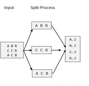
The nature of the computation described previously fits perfectly with this approach. With four processes and 1000 lines to process, each process $i=1,2,3,4$ can be directed to focus on their portion of the file, first can take rows $1,..,250$ , the next can take $251,..,500$ , so on.

Here we present the main processor of the code, called split_process which can determine line beginning and end points in terms of seek byte locations of a given file, and by inspecting the workobj.ci will jump ahead toward the chunk and start reading the file line by line, and feed them into workobj.exec. In an object-oriented design will allow each workobj to know how to handle an input line, will either accumulate results from it or write an output itself to another file.

import os, numpy as np

def split_process(file_name,N,workobj):
    file_size = os.path.getsize(file_name)
    beg = 0
    chunks = []
    for i in range(N):
        with open(file_name, ’r’) as f:
            s = int((file_size / N)*(i+1))
            f.seek(s)
            f.readline()
            end_chunk = f.tell()-1
            chunks.append([beg,end_chunk])
            f.close()
        beg = end_chunk+1
    c = chunks[workobj.ci]
    with open(file_name, ’r’) as f:
        f.seek(c[0])
        while True:
            line = f.readline()
            workobj.exec(line)
            if f.tell() > c[1]: break
        f.close()
        workobj.post()

The results, if they can be accumulated in memory, can be kept on workobj. Once a chunk is finished (all its rows are visited) then split_process will call workobj.post which can handle disk output, cleaning up operations.

The job classes for $A^{T}A$ , $AB$ and random projection are given below.

3.1 Calculation of $A^{T}A$

class ATAJob:
    def __init__(self,D,ci):
        self.C = np.zeros((D,D))
        self.ci = ci
    def exec(self,line):
        tok = line.split(’;’)
        vec = np.array([float(x) for x in tok])
        self.C = self.C + np.outer(vec, vec)
    def post(self):
        outfile = "/tmp/C-%d.csv" % self.ci
        np.savetxt(outfile, self.C, delimiter=’;’,fmt=’%1.6f’)

3.2 Multiplication of $A$ and $B$

class MultJob:
    def __init__(self,ci,bfile):
        self.afile = ""
        self.B = np.loadtxt(bfile,delimiter=’;’)
        self.ci = ci
        cname = "%s/C-%d.csv" % (os.path.dirname(afile), self.ci)
        self.outfile = open(cname, "w")
    def exec(self,line):
        vec = np.array([np.float(x) for x in line.strip().split(";")])
        vec = np.reshape(vec, (len(vec),1))
        res = (vec * self.B).sum(axis=0).tolist()
        res = ";".join(map(str, res))
        self.outfile.write(res)
        self.outfile.write("\n")
        self.outfile.flush()
    def post(self):
        self.outfile.close()

3.3 Random Projection

class RandomProjJob:
    def __init__(self,ci):
        self.ci = ci
        self.k = 7
        self.outfile = open("/tmp/Y-%d.csv" % self.ci, "w")
    def exec(self,line):
        s = np.zeros(self.k)
        toks = line.strip().split(’;’)
        row = np.array([np.float(x) for x in toks[1:]])
        # degisik veri parcalari degisik rasgele matrisler uretsin
        np.random.seed(0)
        for elem in row: s += elem*np.random.normal(0,1,self.k)
        s = ";".join(map(str, s))
        self.outfile.write(s)
        self.outfile.write("\n")
        self.outfile.flush()

    def post(self):
        self.outfile.close()

4 Conclusion

We demonstrated easy-to-scale parallelization approach that can be used on different types of linear algebra problems. A final note here is that the random projection technique, though presented as helping SVD, can also be used in place of SVD [7] as preserving distances between projected rows is useful for any similarity calculation method typically using cosine or Euclidian methods.

References

[1] Gleich, Benson, Demmel, Direct QR factorizations for tall-and-skinny matrices in MapReduce architectures, arXiv:1301.1071 [cs.DC], 2013
[2] N. Halko, Randomized methods for computing low-rank approximations of matrices, University of Colorado, Boulder, 2010
[3] S. Dangupta, A. Gupta An Elementary Proof of a Theorem of Johnson and Lindenstrauss, Wiley Periodicals, 2002
[4] M. Kurucz, A. A. Benczúr, K. Csalogány, Methods for large scale SVD with missing values, ACM, 2007
[5] Zadeh, CME 323: Distributed Algorithms and Optimization, Lecture 17, https://stanford.edu/~rezab/classes/cme323/S17/
[6] Agrawal, Matrix Multiplication: Inner Product, Outer Product and Systolic Array, https://www.adityaagrawal.net/blog/architecture/matrix_multiplication
[7] Lu, On Low Dimensional Random Projections and Similarity Search, https://www.researchgate.net/publication/221615011_On_Low_Dimensional_Random_Projections_and_Similarity_Search