An algorithm for variable density sampling with block-constrained acquisition
Abstract
Reducing acquisition time is of fundamental importance in various imaging modalities. The concept of variable density sampling provides an appealing framework to address this issue. It was justified recently from a theoretical point of view in the compressed sensing (CS) literature. Unfortunately, the sampling schemes suggested by current CS theories may not be relevant since they do not take the acquisition constraints into account (for example, continuity of the acquisition trajectory in Magnetic Resonance Imaging - MRI). In this paper, we propose a numerical method to perform variable density sampling with block constraints. Our main contribution is to propose a new way to draw the blocks in order to mimic CS strategies based on isolated measurements. The basic idea is to minimize a tailored dissimilarity measure between a probability distribution defined on the set of isolated measurements and a probability distribution defined on a set of blocks of measurements. This problem turns out to be convex and solvable in high dimension. Our second contribution is to define an efficient minimization algorithm based on Nesterov’s accelerated gradient descent in metric spaces. We study carefully the choice of the metrics and of the prox function. We show that the optimal choice may depend on the type of blocks under consideration. Finally, we show that we can obtain better MRI reconstruction results using our sampling schemes than standard strategies such as equiangularly distributed radial lines.
Key-words: Compressed Sensing, blocks of measurements, blocks-constrained acquisition, dissimilarity measure between discrete probabilities, optimization on metric spaces.
1 Introduction
Compressive Sensing (CS) is a recently developed sampling theory that provides theoretical conditions to ensure the exact recovery of signals from a few number of linear measurements (below the Nyquist rate). CS is based on the assumption that the signal to reconstruct can be represented by a few number of atoms in a certain basis. We say that the signal is -sparse if
where denotes the pseudo-norm, counting the number of non-zero entries of . Original CS theorems [Don06, CRT06, CP11a] assert that a sparse signal can be faithfully reconstructed via -minimization:
| (1) |
where () is a sensing matrix, represents the vector of linear projections, and for all . More precisely CS results state that measurements are enough to guarantee exact reconstruction provided that satisfies some incoherence property.
One way to construct is by randomly extracting rows from a full sensing matrix that can be written as
| (2) |
where denotes the -th row of . In the context of Magnetic Resonance Imaging (MRI) for instance, the full sensing matrix consists in the composition of a Fourier transform with an inverse wavelet transform. This choice is due to the fact that the acquisition is done in the Fourier domain, while the images to be reconstructed are assumed to be sparse in the wavelet domain. In this setting, a fundamental issue is constructing by extracting appropriate rows from the full sensing matrix . A theoretically founded approach to build (i.e. constructing of sampling schemes) consists in randomly extracting rows from according to a given density. This approach requires to define a discrete probability distribution on the set of integers that represents the indexes of the rows of . We call this procedure variable density sampling. This term appeared in the early MRI paper [SPM95]. It was recently given a mathematical definition in [CCKW13]. One possibility to construct is to choose its i-th component to be proportional to (see [Rau10, PVW11, BBW13, CCW13]) i.e.
| (3) |
In the MRI setting, another strategy ensuring good reconstruction is to choose according to a polynomial radial distribution [KW12] in the so-called k-space i.e. the 2D Fourier plane where low frequencies are centered. Other strategies are possible. For example, [AHPR13] propose a multilevel uniformly random subsampling approach.
All these strategies lead to sampling schemes that are made of a few but isolated measurements, see e.g. Figure 1 (a). However, in many applications, the number of measurements is not of primary importance relative to the path the sensor must take to collect the measurements. For instance, in MRI, sampling is done in the Fourier domain along continuous and smooth curves [Wri97, LKP08]. Another example of the need to sample continuous trajectories can be found in mobile robots monitoring where robots have to spatially sample their environment under kinematic and energy consumption constraints [HPH+11].
This paper focuses on the acquisition of linear measurements in applications where the physics of the sensing device allows to sample a signal from pre-defined blocks of measurements. We define a block of measurements as an arbitrary set of isolated measurements, that could be contiguous in the Fourier plane for instance. As an illustrative example (that will be used throughout the paper), one may consider sampling patterns generated by randomly drawing a set of straight lines in the Fourier plane or k-space as displayed in Figure 1(b). This kind of sampling patterns is particularly relevant in the case of MRI acquisition with echo planar sampling strategies, see e.g. [LDSP08].
Acquiring data by blocks of measurements raises the issue of designing appropriate sampling schemes. In this paper, we propose to randomly extract blocks of measurements that are made of several rows from the full sensing matrix . The main question investigated is how to choose an appropriate probability distribution from which blocks of measurements will be drawn. A first step in this direction [BBW13, PDG12] was recently proposed. In [BBW13], we have derived a theoretical probability distribution in the case of blocks of measurements to design a sensing matrix that guarantees an exact reconstruction of -sparse signals with high probability. Unfortunately, the probability distributions proposed in [BBW13] and [PDG12] are difficult to compute numerically and seem suboptimal in practice.
In this paper, we propose an alternative strategy which is based on the numerical resolution of an optimization problem. Our main idea is to construct a probability distribution on a dictionary of blocks. The blocks are drawn independently at random according to this distribution. We propose to choose in such a way that the resulting sampling patterns are similar to those based on isolated measurements, such as the ones proposed in the CS literature. For this purpose, we define a dissimilarity measure to compare a probability distribution on a dictionary of blocks and a target probability distribution defined on a set of isolated measurements. Then, we propose to choose an appropriate distribution by minimizing its dissimilarity with a distribution on isolated measurements that is known to lead to good sensing matrices.
This paper is organized as follows. In Section 2, we introduce the notation. In Section 3, we describe the problem setting. Then, we construct a dissimilarity measure between probability distributions lying in different, but spatially related domains. We then formulate the problem of finding a probability distribution on blocks of measurements as a convex optimization problem. In Section 4, we present an original and efficient way to solve this minimization problem via a dual formulation and an algorithm based on the accelerated gradient descents in metric spaces [Nes05]. We study carefully how the theoretical rates of convergence are affected by the choice of norms and prox-functions on the primal and dual spaces. Finally, in Section 5, we propose a dictionary of blocks that is appropriate for MRI applications. Then, we compare the quality of MRI images reconstructions using the proposed sampling schemes and those currently used in the context of MRI acquisition, demonstrating the potential of the proposed approach on real scanners.
 |
 |
| (a) | (b) |
2 Notation
We consider -dimensional signals for any , of size . Let and denote finite-dimensional vector spaces endowed with their respective norms and . In the paper, we identify to and to . We denote by and , respectively the dual spaces of and . For and we denote by the value of at . The notation will denote the usual inner product in a Euclidean space. The norm of the dual space is defined by:
Let denote some operator. When is linear, we denote its adjoint operator by . The subordinate operator norm is defined by :
When the spaces and are endowed with and norms respectively, we will use the following notation for the operator norm of :
We set to be the simplex in , and to be the simplex in . For and an index we denote by the -th component of .
Let denote a closed convex function. Its Fenchel conjugate is denoted . The relative interior of a set is denoted . Finally, the normal cone to at a point on the boundary of is denoted .
3 Variable density sampling with block constraints
3.1 Problem setting
In this paper, we assume that the acquisition system is capable of sensing a finite set of linear measurements of a signal such that
where denotes the -th row of the full sensing matrix . Let us define a set where each denotes a set of indexes. We assume that the acquisition system has physical constraints that impose sensing simultaneously the following sets of measurements
In what follows, we refer to as the blocks dictionary.
For example in MRI, is the number of pixels or voxels of a 2D or 3D image, and represents the -th discrete Fourier coefficient of this image. In this setting, the sets of indexes may represent straight lines in the discrete Fourier domain as in Figure 1(b). In Section 5.1, we give further details on the construction of such a dictionary.
We propose to partially sense the signal using the following procedure:
- (i)
Construct a discrete probability distribution .
- (ii)
Draw i.i.d. indexes from the probability distribution on the set , with .
- (iii)
Sense randomly the signal by considering the random set of blocks of measurements , which leads to the construction of the following sensing matrix
The main objective of this paper is to provide an algorithm to construct the discrete probability distribution based on the knowledge of a target discrete probability distribution on the set of isolated measurements. The problem of choosing a distribution leading to good image reconstruction is not addressed in this paper, since there already exist various theoretical results and heuristic strategies in the CS literature on this topic [LKP08, CCW13, AHPR13, KW12].
3.2 A variational formulation
In order to define , we propose to minimize a dissimilarity measure between and . The difficulty lies in the fact that these two probability distributions belong to different spaces. We propose to construct a dissimilarity measure that depends on the blocks dictionary . This dissimilarity measure will be minimized over using numerical algorithms with being relatively large (typically ). Therefore, it must have appropriate properties such as convexity, for the problem to be solvable in an efficient way.
Mapping the -dimensional simplex to the -dimensional one
In order to define a reasonable dissimilarity measure, we propose to construct an operator that maps a probability distribution to some :
where for ,
| (4) |
where is equal to 1 if , 0 otherwise. The -th element of represents the probability to draw the -th measurement by drawing blocks of measurements according to the probability distribution . The operator satisfies the following property by construction :
A sufficient condition for the mapping to be a linear operator
Note that the operator is generally non linear, due to the denominator in (4). This is usually an important drawback for the design of numerical algorithms involving the operator . However, if the sets all have the same cardinality (or length) equal to , the denominator in (4) is equal to . In this case, becomes a linear operator. In this paper, we will focus on this setting, which is rich enough for many practical applications:
Assumption 3.1.
For , , where is some positive integer.
Let us provide two important results for the sequel.
Proposition 3.2.
For , , i.e. is a strict subset of .
Proof.
By definition of the convex envelope, , where denotes the -th column of . For , is a subset of that does not contain the extreme points of the simplex.
In practice, Proposition 3.2 means that it is impossible to reach exactly an arbitrary distribution , except for the trivial case of isolated measurements.
Proposition 3.3.
Suppose that Assumption 3.1 holds, then for ,
Proof.
Under Assumpiton 3.1, all the columns of have only non-zero coefficients equal to . With , we can thus derive that
where denotes the -th column of , and is the conjugate of satisfying .
Measuring the dissimilarity between and through the operator
Now that we have introduced the mapping , we propose to define a dissimilarity measure between and . To do so, we propose to compare and that are both vectors belonging to the simplex . Owing to Proposition 3.2, it is hopeless to find some satisfying for an arbitrary target density . Therefore, we can only expect to get an approximate solution by minimizing a dissimilarity measure . For obvious numerical reasons, should be convex in . Among statistical distances, the most natural ones are the total variation distance, Kullback-Leibler of more generally f-divergences. Among this family, total variation presents the interest of having a dual of bounded support. We will exploit this property to design efficient numerical algorithms in Section 4. In the sequel, we will thus use to compare the distributions and .
Entropic regularization
In applications such as MRI, the number of columns of is larger than the number of its rows. Therefore, and there exist multiple with the same dissimilarity measure . In this case, we propose to take among all these solutions, the one minimizing the neg-entropy defined by
| (5) |
with the convention that . We recall that the entropy is proportional to the Kullback-Leibler divergence between and the uniform distribution in (i.e. such that for all ). Therefore, among all the solutions minimizing , choosing the distribution minimizing gives priority to entropic solutions, i.e. probability distributions which maximize the covering of the sampling space if we proceed to several drawings of blocks of measurements. Therefore, we can finally write the following regularized problem defined by
| (PP) |
where
for some regularization parameter . Adding the neg-entropy has the effect of spreading out the probability distribution , which is a desirable property. Moreover, the neg-entropy is strongly convex on the simplex . This feature is of primary importance for the numerical resolution of the above optimization problem. Note that an appropriate choice of the regularization parameter is also important, but this issue will not be addressed in this paper.
A toy example
To illustrate the interest of Problem (PP), we design a simple example. Consider a image. Define the target distribution as a dirac on the central pixel (numbered 5 in Figure 2). Consider a blocks dictionary composed of horizontal and vertical lines. In that setting, the operator is given by
For such a matrix, there are various distributions minimizing . For example, one can choose or . The solution maximizing the entropy is . In the case of image processing, this solution is preferable since it leads to better covering of the acquisition space. Note that, among all the -norms (, only the -norm is such that . This property is once again desirable since we want the regularizing term (and not the fidelity term) to force choosing the proper solution.
4 Optimization
In this section, we propose a numerical algorithm to solve Problem (PP). Note that despite being convex, this optimization problem has some particularities that make it difficult to solve. Firstly, the parameter lies in a very high dimensional space. In our experiments, varies between and while varies between and . Moreover, the function is differentiable but its gradient is not Lipschitz, and the total variation distance is non-differentiable.
The numerical resolution of Problem (PP) is thus a delicate issue. Below, we propose an efficient strategy based on the numerical optimization of the dual problem of (PP), and on the use of Nesterov’s ideas [Nes05]. Contrarily to most first order methods proposed recently in the literature [BC11, Nes13, CDV10] which are based on Hilbert space formalisms, Nesterov’s algorithm is stated in a (finite dimensional) normed space. We thus perform the minimization of the dual problem on a metric space, and we carefully study the optimal choice of the norms in the primal and dual spaces. We show that depending on the blocks length , the optimal choice might well be different from the standard -norm. Such ideas stem back from (at least) [CT93], but were barely used in the domain of image processing.
4.1 Dualization of the problem
Our algorithm consists in solving the problem dual to (PP) in order to avoid the difficulties related to the non-differentiability of the -norm. Proposition 4.1 and 4.3 state that the dual of problem (PP) is differentiable. We will use this feature to design an efficient first-order algorithm and use the primal-dual relationships (Proposition 4.4) to retrieve the primal solution.
Proposition 4.1.
Let for . The dual problem to (PP) is:
| (DP) |
in the sense that , where is the -ball of unit radius in .
Proof.
The proof is available in Appendix A.
In order to study the regularity properties of , and so the solvability of (DP), we use the strong convexity of the neg-entropy with respect to . First, let us recall one version of the definition of the strong convexity in Banach spaces.
Definition 4.1.
We say that is -strongly convex with respect to on if
| (6) |
We define the convexity modulus of as the largest positive real satisfying Equation (6).
Proposition 4.2.
For , , the convexity modulus of the neg-entropy on the simplex is .
Proof.
The proof is available in Appendix B.
Proposition 4.3.
The function is convex and its gradient is Lipschitz continuous i.e.
with constant
| (7) |
Moreover, is locally Lipschitz around with constant
| (8) |
where is the local convexity modulus of around , and an explicit expression for is given in (19).
Proof.
The proof is available in Appendix C.
Note that a standard reasoning would rather lead to , which is usually much larger than bound (7). Proposition 4.3 implies that Problem (DP) is efficiently solvable by Nesterov’s algorithm [Nes05]. Therefore, we will first solve the dual problem (DP). Then, we use the relationships between the primal and dual solutions (as described in Proposition 4.4) to finally compute a primal solution for Problem (PP).
Proposition 4.4.
The relationships between the primal and dual solutions
are given by
| (9) |
Furthermore,
| (10) |
4.2 Numerical optimization of the dual problem
Now that the dual problem (DP) is fully characterized, we propose to solve it using Nesterov’s optimal accelerated projected gradient descent [Nes05] for smooth convex optimization.
4.2.1 The algorithm
Nesterov’s algorithm is based on the choice of a prox-function of the set , i.e. a continuous function that is strongly convex on w.r.t. . Let denote the convexity modulus of , we further assume that so that
where . Nesterov’s algorithm is described in Algorithm 1.
Theorem 4.5.
Since is generally unknown, we can bound (11) by
| (12) |
where . Note that until now, we got theoretical guarantees in the dual space but not in the primal. What matters to us is rather to obtain guarantees on the primal iterates, which can be summarized by the following theorem.
Theorem 4.6.
The proof is given in Appendix D. It is a direct consequence of a more general result of independent interest.
4.2.2 Choosing the prox-function and the metrics
Algorithm 1 depends on the choice of , and . The usual accelerated projected gradient descents consist in setting , and . However, we will see that it is possible to change the algorithm’s speed of convergence by making a different choice. In this paper we concentrate on the usual -norms, .
Choosing a norm on :
The following proposition shows an optimal choice for .
Proposition 4.7.
The norm that minimizes (12) among all -norms, is . Note however that the minimum local Lipschitz constant for might be reached for another choice of .
Proof.
From Proposition 4.2, we get that remains unchanged no matter how is chosen among -norms. The choice of is thus driven by the minimization of . From the operator norm definition, it is clear that the best choice consists in setting since the -norm is the smallest of all -norms.
Choosing a norm on and a prox-function :
by Proposition 4.7 the norm and the prox function should be chosen in order to minimize . We are unaware of a general theory to make an optimal choice despite recent progresses in that direction. The recent paper [dJ13] proposes a systematic way of selecting and in order to make the algorithm complexity invariant to change of coordinates for a general optimization problem. The general idea in [dJ13] is to choose to be the Minkowski gauge of the constraints set (of the optimization problem), and to be a strongly convex approximation of . However, this strategy is not shown to be optimal. In our setting, since the constraints set is , this would lead to choose . Unfortunately, there is no good strongly convex approximation of .
In this paper, we thus study the influence of and both theoretically and experimentally, with . Propositions 4.8, 4.9 and 4.10 summarize the theoretical algorithm complexity in different regimes.
Proposition 4.8.
Let . Define . Then
- •
For , is -strongly convex w.r.t. .
- •
For , is -strongly convex w.r.t. .
Proof.
Proposition 4.9.
Proof.
The result is a direct consequence of Proposition 4.8.
Unfortunately, the bounds in (13), (14) and (15) are dimension dependent. Moreover, the optimal choice suggested by Proposition 4.9 is different from the Minkowski gauge approach suggested in [dJ13]. Indeed, in all the cases described in Proposition 4.5, the optimal choice differs from . The difficulty to apply this approach is to find a function strongly convex w.r.t. . A simple choice consists in setting . This function is -strongly convex w.r.t. . We thus get the following proposition:
Proposition 4.10.
4.3 Numerical experiments on convergence
In this section, we are willing to emphasize the improvement achieved by appropriately choosing the norms , , and the prox-function . To do so, we run experiments on a dictionary of blocks of measurements having all the same size , described in Section 5.1, for 2D images of size . At first, we choose , and and we perform Algorithm 1 for this dictionary. In fact, this first case (the norm on E differs from the usual ) nearly corresponds to a standard accelerated gradient descent [NN04]. In a second time, we set , . In Figure 3, we display the decrease of the objective function in both settings. Figure 3 points out that a judicious selection of norms on and can significantly speed up the convergence: for 29 000 iterations, the standard accelerated projected gradient descent reaches a precision of whereas Algorithm 1 with , , i.e. a ”modified” gradient descent, reaches a precision of . The conclusions for this numerical experiment appear to be faithful to what was predicted by the theory, see Proposition 4.5. For the sake of completeness, we add in Figure 3 (in green) the case where , and , which is an usual choice in practice. Clearly, this is the slowest rate of convergence observed.
Finally, we perform the algorithm for , , and by changing the value of . The value of provided by Proposition 4.3 is tight uniformly on . However, the local Lipschitz constant of varies rapidly inside the domain. In practice, the Lipschitz constant around the minimizer may be much smaller than (note that for all ). In this last heuristic approach, we will decrease by substantial factors without losing practical convergence. This result is presented in Figure 3 where the black curve denotes convergence result when the Lipschitz constant has been divided by 100. We can observe that in this case, it suffices 1500 iterations to reach the precision obtained by the case , and (in red) after 29000 iterations. Let us give an intuitive explanation to this positive behaviour. To simplify the reasoning, let us assume that is the uniform probability distribution. First notice that the choice of only influences the Lipschitz constant of but does not change the algorithm, so that we can play with the norm on to decrease the local Lipschitz constant. Furthermore, the choice of minimizing the global Lipschitz constant may be different from the one minimizing the local Lipschitz constant. Considering that , from Equation (8), we get that . Using Perron-Frobenius theorem, it can be shown that for our choice of dictionary, and for . From this simple reasoning, we can conclude that the local Lipschitz constant around is no greater than . This means that if the minimizer is sufficiently far away from the simplex boundary, we can decrease by a significant factor without loosing convergence.

5 Numerical results
In this section, we assess the reconstruction performance of the sampling patterns using the approach described in Section 4.2 with . We compare it to standard approaches used in the context of MRI. We call the probability distribution resulting from the minimization problem (PP) for a given target distribution on isolated measurements.
5.1 The choice of a particular dictionary of blocks
From a numerical point of view, we study a particular system of blocks of measurements. The dictionary used in all numerical experiments of this article is composed of discrete lines of length , joining any pixel on the edge of the image to any pixel on the opposite edge, as in Figure 1(b). Note that the number of blocks in this dictionary is for an image of size . The choice of such a dictionary is particularly relevant in MRI, since the gradient waveforms that define the acquisition paths is subject to bounded-gradient and slew-rate constraints, see e.g. [LKP08]. Moreover the practical implementation on the scanner of straight lines is straightforward since it is already in use in standard echo-planar imaging strategies.
Remark that, in such a setting, the mapping , defined in (4), is a linear mapping that can be represented by a matrix of size with when the -th pixel belongs to the -th block, for and .
One may argue that in MRI, dealing with samples lying on continuous lines (and not discrete grids) is more realistic in the design of the MR sequences. To deal with this issue, one could resort to the use of the Non-Uniform Fast Fourier Transform. This technique is however much more computationally intensive. In this paper we thus stick to values of the Fourier transform located on the Euclidean grid. This is commonly used in MRI with regridding techniques.
5.2 The reconstructed probability distribution
We are willing to illustrate the fidelity of , the solution of Problem (PP), to a given target . In the setting of 2D MR sensing, with the dictionary of lines in dimension described in the previous subsection. We set the target probability distribution the one suggested by current CS theories on the set of isolated measurements. It is proportional to , see [PVW11, CCW13, BBW13]. To give an idea of what the resulting probability distribution looks like, we draw 100 000 independent blocks of measurements according to and count the number of measurement for each discrete Fourier coefficient. The result is displayed on Figure 4. This experiment underlines that our strategy manages to catch the overall structure of the target probability distibution.
 |
 |
| (a) | (b) |
5.3 Reconstruction results
In this section, we compare the reconstruction quality of MR images for different acquisition schemes. The comparison is always performed for schemes with an equivalent number of isolated measurements. We recall that in the case of MR images, the acquisition is done in the Fourier domain, and MR images are supposed to be sparse in the wavelet domain. Therefore, the full sensing matrix , which models the acquisition process, is the composition of a Fourier transform with an inverse Wavelet transform. The reconstruction is done via -minimization as presented in (1), using Douglas-Rachford algorithm [CP11b]. It was proven in various papers [CCW13, CCKW13, AHPR13] that MRI image quality can be strongly improved by fully acquiring the center of the Fourier domain via a mask defined by the support of the mother wavelet, see Figure 5. Therefore, for every type of schemes used in our reconstruction test, we first fully acquire this mask.
 |
 |
| (a) | (b) |
The various schemes considered in this paper are based on blocks of measurements and on heuristic schemes that are widely used in the context of MRI. They will consist in:
- •
Equiangularly distributed radial lines: the scheme is made of lines always intersecting the center of the acquisition domain, and that are distributed uniformly [LDSP08].
- •
Golden angle scheme: the scheme is made of radial lines separated from the golden angle, i.e . This technique is used often in MRI sequences, and it gives good reconstruction results in practice [WSK+07].
- •
Random radial scheme: radial lines are drawn uniformly at random [CRCP12].
- •
Scheme based on the dictionary described in Section 5.1
- –
Blocks are drawn according to which is the resulting probability distribution obtained by minimizing Problem (PP) for . The distribution a radial distribution that decreases as . This choice was justified recently in [KW12] and used extensively in practice. Note that is set to on the -space center since it is already sampled deterministically, see Figure 6 (b).
- –
- –
 |
 |
| (a) | (b) |
 |
 |
| (a) Brain | (b) Baboon |
Setting
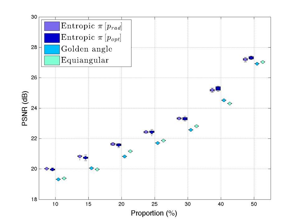
The numerical experiment is run for images of size with . The full dictionary described in Section 5.1 contains lines of length pixels connecting every point on the edge of the image to every point on the opposite side. For each proportion of measurements (), we proceed to drawings of schemes when the considered scheme is random. Reconstruction results, for the reference images showed in Figure 7 and for various sampling schemes, are displayed in the form of boxplots of PSNR in Figure 8 (a)(c).
 |
 |
|---|---|
| (a) Brain in | (b) Brain in |
 |
 |
| (c) Baboon in | (d) Baboon in |
Figure 8 shows that the schemes based on the approach presented in this article give better results than random radial schemes, for any proportion of measurements. The improvement in terms of PSNR is generally between and dB. The schemes based on and are competitive with those based on the golden angle or equiangularly distributed schemes in the case where the proportion of measurements is low (less than of measurements). We observe that for measurements, schemes based on our dictionary and drawn according to outperform by more than dB the standard sampling strategies. Increasing the PSNR of dB is significant and can be qualitatively observed in the reconstructed image.
Figures 8(a) and (c) allow to compare the quality of the reconstructions using different sampling schemes and different undersampling ratios. In this experiment, it can be seen that block-constrained acquisition never outperforms acquisitions based on indepenedent measurements. This was to be expected since adding constraints reduces the space of possible sampling patterns. Once again, note that independent drawings are however not conceivable in many contexts such as MRI. In Figures 8(a) and (c), it can also be seen that the proposed sampling approach always produces results comparable to the standard sampling schemes and tend to produce better results for low sampling ratios.
Finally, in Figure 9, we illustrate that block-constrained acquisition does not allow to reach an arbitrary target distribution by showing the difference between and the probability distribution which is defined on the set of isolated measurements. This confirms Proposition 3.2 experimentally.
 |
 |
| (a) | (b) |
Setting
Given that in CS the quality of the reconstruction can be resolution dependent, as described in [AHPR13], we have decided to run the same numerical experiment on images. The numerical experiment is run for images of size with . The full dictionary described in Section 5.1 contains lines of length connecting every point on the edge of the image to every point on the opposite side. For each proportion of measurements (), we proceed to drawings of sampling schemes when the considered scheme is random. The images of reference to reconstruct are the same as in the setting , see Figure 7.
 |
 |
| (a) PSNR = 40.1364 dB | (b) PSNR = 41.8854 dB |
 |
 |
| (c) | (d) |
Quality of reconstructions are compared in Figure 8(b) and (d) for the golden or equiangularly distributed lines and our proposed method based on and . This experiment shows that the PSNR of the reconstructed images is significantly improved by using the proposed method until of measurements for the brain image and until of measurements for the baboon one. We can remark that for both images, for a same proportion of measurements, the PSNR of the reconstructed images increases while the resolution increases. This numerical experiment suggests that the proposed sampling approach might be significantly better than traditional ones in the MRI context for high resolution images. In Figure 10 (a), we present the reconstructed image of the brain from of measurements in the case of a golden angle scheme. In Figure 10 (b), we present the reconstructed image of the brain from of measurements in the case of a realization of schemes based on . The latter’s PSNR is 41.88 dB whereas in the golden scheme case, the PSNR only reaches 40.13 dB. In Figure 10 (c) and (d), we display the corresponding difference images to the reference image, which underlines the improvement of 1.7 dB in our method.
As a side remark, let us mention that in MRI, sampling diagonal or horizontal lines actually takes the same scanning time (even though the diagonals are longer), since gradient coils work independently in each direction. In the MRI example, the length of the path is thus less meaningful that the number of scanned lines. In Figure 11, we show different sampling schemes based on the golden angle pattern or on our method with the same number of lines, and we show the corresponding reconstructions of brain images.
 |
 |
| (a) Golden angle scheme (9.2%) | (b) -based scheme (10%) |
 |
 |
| (c) PSNR = 36.34 dB | (d) PSNR = 38.99 dB |
 |
 |
| (e) Golden angle | (f) -based scheme |
Remark.
In both settings, for the brain image, schemes based on lead to better reconstruction results in terms of PSNR than schemes from . This can be explained by the fact that is the probability density given by CS theory which provides guarantees for any -sparse image to reconstruct. However, brain images or natural images have a structured sparsity in the wavelet domain: indeed, their wavelet transform is not uniformly -sparse, the approximation part contains more non-zero coefficients than the rest of the details parts. We can infer that manages to catch the sparsity structure of the wavelet coefficients of the considered images.
6 Conclusion
In this paper, we have focused on constrained acquisition by blocks of measurements. Sampling schemes are constructed by drawing blocks of measurements from a given dictionary of blocks according to a probability distribution that needs to be chosen in an appropriate way. We have presented a novel approach to compute in order to imitate existing sampling schemes in CS that are based on the drawing of isolated measurements. For this purpose, we have defined a notion of dissimilarity measure between a probability distribution on a dictionary of blocks and a probability distribution on a set of isolated measurements. This setting leads to a convex minimization problem in high dimension. In order to compute a solution to this optimization problem, we proposed an efficient numerical approach based on the work of [Nes05]. Our numerical study highlights the fact that performing minimization on a metric space rather than a Hilbert space might lead to significant acceleration. Finally, we have presented reconstruction results using this new approach in the case of MRI acquisition. Our method seems to provide better reconstruction results than standard strategies used in this domain. We believe that this last point brings interesting perspectives for 3D MRI reconstruction.
As an outlook, we plan to extend the proposed numerical method to a wider setting and to provide better theoretical guarantees for cases where the Lipschitz constant of the gradient may vary across the domain. A first step in this direction was proposed recently in [GK13]. We also plan to accelerate the matrix-vectors product involving by using fast Radon transforms. This step is unavoidable to apply our algorithm in 3D or 3D+t problems for which we expect important benefits compared to the small images we tested until now. Finally we are currently collaborating with physicists at Neurospin, CEA and plan to implement the proposed sampling schemes on real MRI scanners.
Acknowledgement
The authors wish to thank Jean-Baptiste Hiriart-Urruty, Fabrice Gamboa and Alexandre Vignaud for fruitful discussion. They also thank the referees for their remarks which helped clarifying the paper. This work was partially supported by the CIMI (Centre International de Mathématiques et d’Informatique) Excellence program, by ANR SPH-IM-3D (ANR-12-BSV5-0008), by the FMJH Program Gaspard Monge in optimization and operation research, and by the support to this program from EDF.
Appendix A Proof of Proposition 4.1
First, we express the Fenchel-Rockafellar dual problem [Roc97]:
where stands for the -ball of unit radius and
| (16) |
The solution of the minimization problem (16) satisfies
| (17) |
where denotes the normal cone to the set at the point , and denotes the relative interior of . Equation (17) can be rewritten in the following way
| (18) |
By choosing and plugging it into (18) we get that
| (19) |
It remains to plug (19) in (16) to obtain (DP) with
Appendix B Proof of Proposition 4.2
The neg-entropy is continuous, and twice continuously differentiable on . Then, in order to prove its strong convexity, it is sufficient to bound from below its positive diagonal Hessian with respect to . We have
| (20) |
Using Cauchy-Schwartz’s inequality,
Therefore, is -strongly convex on the simplex with respect to . Since for all , , we get:
Moreover if denotes a sequence of pointwise converging to the first element of the canonical basis and , then
so that the inequality is tight.
Appendix C Proof of Proposition 4.3
The proof is based on similar arguments as [Nes05, Theorem 1]. First, notice that
| (21) |
where
is the local convexity modulus of on the segment .
Next, recall that
The optimality conditions of the previous maximization problem for and , , lead to
Combining the two previous inequalities, we can write that for :
Therefore, we can write that
Noting that , we can conclude that
Let us consider a sequence converging uniformly towards . Since is a continuous mapping, converges uniformly towards . Thus,
Appendix D Proof of Theorem 4.6
Theorem 4.6 is a direct consequence of Lemma (D.1) below. A similar proof was proposed in [FP11], but not extended to a general setting.
Lemma D.1.
Proof.
Point (i) is a standard result in convex analysis. See e.g. [HUL96]. We did not find the result (ii) in standard textbooks and to our knowledge it is new. We assume for simplicity that , , and are differentiable. This hypothesis is not necessary and can be avoided at the expense of longer proofs. First note that
by Fenchel-Rockafellar duality. Since is strongly convex is a one-to-one mapping and
| (25) |
The primal-dual relationships read
So that
Let us define the following Bregman divergences quantities:
By construction
Moreover since is the minimizer of it satisfies . By replacing this expression in and using the fact that is convex we get that
We now have all the ingredients to prove Theorem 4.6.
Proof of Theorem 4.6.
The proof is a direct consequence of Lemma D.1. It can be obtained by setting , and , with the indicator function of the set . Thus and . Then remark that defined in Theorem 4.6 satisfies . By Proposition 4.2, we get that is -strongly convex w.r.t. , for all . It then suffices to use bound (12) together with Lemma D.1 to conclude.
References
- [AHPR13] Ben Adcock, Anders C Hansen, Clarice Poon, and Bogdan Roman. Breaking the coherence barrier: asymptotic incoherence and asymptotic sparsity in compressed sensing. arXiv preprint arXiv:1302.0561, 2013.
- [BBW13] Jérémie Bigot, Claire Boyer, and Pierre Weiss. An analysis of block sampling strategies in compressed sensing. Preprint, 2013.
- [BC11] Heinz H Bauschke and Patrick L Combettes. Convex analysis and monotone operator theory in Hilbert spaces. Springer, 2011.
- [CCKW13] Nicolas Chauffert, Philippe Ciuciu, Jonas Kahn, and Pierre. Weiss. Variable density sampling with continuous sampling trajectories. preprint, 2013.
- [CCW13] Nicolas Chauffert, Philippe Ciuciu, and Pierre Weiss. Variable density compressed sensing in MRI. theoretical vs heuristic sampling strategies. In proceedings of IEEE ISBI, 2013.
- [CDV10] Patrick L Combettes, Đinh Dũng, and Bằng Công Vũ. Dualization of signal recovery problems. Set-Valued and Variational Analysis, 18(3-4):373–404, 2010.
- [CP11a] Emmanuel J. Candes and Yaniv Plan. A probabilistic and ripless theory of compressed sensing. Information Theory, IEEE Transactions on, 57(11):7235–7254, 2011.
- [CP11b] Patrick L Combettes and Jean-Christophe Pesquet. Proximal splitting methods in signal processing. In Fixed-Point Algorithms for Inverse Problems in Science and Engineering, pages 185–212. Springer, 2011.
- [CRCP12] Rachel W Chan, Elizabeth A Ramsay, Edward Y Cheung, and Donald B Plewes. The influence of radial undersampling schemes on compressed sensing reconstruction in breast mri. Magnetic Resonance in Medicine, 67(2):363–377, 2012.
- [CRT06] Emmanuel J Candès, Justin Romberg, and Terence Tao. Robust uncertainty principles: Exact signal reconstruction from highly incomplete frequency information. Information Theory, IEEE Transactions on, 52(2):489–509, 2006.
- [CT93] G. Chen and M. Teboulle. Convergence analysis of a proximal-like minimization algorithm using bregman functions. SIAM Journal on Optimization, 3(3):538–543, 1993.
- [dJ13] Alexandre d’Aspremont and Martin Jaggi. An optimal affine invariant smooth minimization algorithm. arXiv preprint arXiv:1301.0465, 2013.
- [Don06] David Donoho. Compressed sensing. Information Theory, IEEE Transactions on, 52(4):1289–1306, 2006.
- [FP11] Jalal M Fadili and Gabriel Peyré. Total variation projection with first order schemes. Image Processing, IEEE Transactions on, 20(3):657–669, 2011.
- [GK13] Clóvis C Gonzaga and Elizabeth W Karas. Fine tuning nesterov’s steepest descent algorithm for differentiable convex programming. Mathematical Programming, pages 1–26, 2013.
- [HPH+11] Robert Hummel, Sameera Poduri, Franz Hover, Urbashi Mitra, and Guarav Sukhatme. Mission design for compressive sensing with mobile robots. In Robotics and Automation (ICRA), 2011 IEEE International Conference on, pages 2362–2367. IEEE, 2011.
- [HUL96] Jean-Baptiste Hiriart-Urruty and Claude Lemaréchal. Convex Analysis and Minimization Algorithms: Part 1: Fundamentals, volume 1. Springer, 1996.
- [JN08] Anatoli Juditsky and Arkadii S Nemirovski. Large deviations of vector-valued martingales in 2-smooth normed spaces. arXiv preprint arXiv:0809.0813, 2008.
- [KW12] Felix Krahmer and Rachel Ward. Beyond incoherence: stable and robust sampling strategies for compressive imaging. arXiv preprint arXiv:1210.2380, 2012.
- [LDSP08] Michael Lustig, David L. Donoho, Juan M. Santos, and John M. Pauly. Compressed sensing mri. Signal Processing Magazine, IEEE, 25(2):72–82, 2008.
- [LKP08] Michael Lustig, Seung-Jean Kim, and John M Pauly. A fast method for designing time-optimal gradient waveforms for arbitrary k-space trajectories. Medical Imaging, IEEE Transactions on, 27(6):866–873, 2008.
- [Nes05] Yurii Nesterov. Smooth minimization of non-smooth functions. Mathematical Programming, 103(1):127–152, 2005.
- [Nes13] Yu. Nesterov. Gradient methods for minimizing composite functions. Mathematical Programming, 140(1):125–161, 2013.
- [NN04] Yurii Nesterov and I͡U E Nesterov. Introductory lectures on convex optimization: A basic course, volume 87. Springer, 2004.
- [PDG12] Adam C Polak, Marco F Duarte, and Dennis L Goeckel. Performance bounds for grouped incoherent measurements in compressive sensing. arXiv preprint arXiv:1205.2118, 2012.
- [PVW11] Gilles Puy, Pierre Vandergheynst, and Yves Wiaux. On variable density compressive sampling. Signal Processing Letters, IEEE, 18(10):595–598, 2011.
- [Rau10] Holger Rauhut. Compressive sensing and structured random matrices. Theoretical foundations and numerical methods for sparse recovery, 9:1–92, 2010.
- [Roc97] R Tyrell Rockafellar. Convex analysis, volume 28. Princeton university press, 1997.
- [SPM95] D. M. Spielman, J. M. Pauly, and C. H. Meyer. Magnetic resonance fluoroscopy using spirals with variable sampling densities. Magnetic resonance in medicine, 34(3):388–394, 1995.
- [Wri97] Graham A. Wright. Magnetic resonance imaging. Signal Processing Magazine, IEEE, 14(1):56–66, 1997.
- [WSK+07] Stefanie Winkelmann, Tobias Schaeffter, Thomas Koehler, Holger Eggers, and Olaf Doessel. An optimal radial profile order based on the golden ratio for time-resolved mri. Medical Imaging, IEEE Transactions on, 26(1):68–76, 2007.