Signal Reconstruction from Rechargeable Wireless Sensor Networks using Sparse Random Projections
Abstract
Due to non-homogeneous spread of sunlight, sensing nodes possess non-uniform energy budget in rechargeable Wireless Sensor Networks (WSNs). An energy-aware workload distribution strategy is therefore necessary to achieve good data accuracy subject to energy-neutral operation. Our previously proposed Energy Aware Sparse approximation Technique (EAST) can approximate a signal, by adapting sensor node sampling workload according to solar energy availability. However, the major shortcoming of EAST is that it does not guarantee an optimal sensing strategy. In other words EAST offers energy neutral operation, however it does not offer the best utilization of sensor node energy, which compromises the reconstruction accuracy. In order to overcome this shortcoming, we propose EAST+ which, maximizes the reconstruction accuracy subject to energy neutral operations. We also propose a distributed algorithm for EAST+, which offers accurate signal reconstruction with limited node to-base communications.
Index Terms:
Rechargeable Wireless Sensor Networks, Sparse Approximation, Energy-aware Sensing, Energy-neutral Operations.I Introduction
Wireless Sensor Networks (WSNs) are currently deployed to monitor micro-climate data from different environments [1, 2]. The Springbrook National Park WSN is one such example [2]. The Springbrook site is part of a World Heritage precinct in Queensland, Australia. CSIRO11 1 The Commonwealth Scientific and Industrial Research Organization, in partnership with the Queensland Government Environmental Protection Agency (EPA), has deployed a WSN of nodes at Springbrook in . This partnership aims to collect microclimate data for enhancing knowledge of the rain forest restoration process.
Energy supply is a major design constraint in the Springbrook deployment. In the last few years, a large number of research has been conducted (see [3] for the comprehensive list) to reduce the radio’s duty cycle. However, recently it has been reported that many real life applications require specific sensors whose power consumption is significant. In addition, longer acquisition times of some specific sensors may even result in significantly higher energy consumptions than the radio transceiver. In order to cope with the increasing energy demand, a number of sensor deployments are adopting a complementary approach of supplementing the energy supply of the system by harvesting additional energy from the environment [2, 4, 5, 6].
Out of the variety of energy harvesting modalities, we use solar energy harvesting modality. Solar energy provides one of the highest power densities [7], however, sun light is not homogeneously spread over the network, which results in non-homogeneous energy level in the sensing nodes. Therefore, a sensing task allocation technique that assumes uniform energy profile of the sensing nodes could deplete the energy of a number of nodes and create holes in the network connectivity or coverage. In order to avoid such situation, an early attempt in the Springbrook deployment reduces the fraction of time the sensors are turned on to take samples (we refer this quantity as sensor on-time) to less than for all nodes, which results in poor approximation of the signal.
Data collected from wireless sensor deployments are typically correlated and therefore compressible [8] in an appropriate transform. If the data is compressible, a signal vector with data values can be well approximated using only orthonormal transform coefficients. If these largest coefficients could be determined from a small number of measurements, where measurements are collected with high probability from energy-rich sensing nodes and with smaller probability from energy-constrained nodes, we can approximate the signal with good accuracy at energy neutral condition. An energy neutral operation means that the energy consumption should be less than the energy harvested from the environment. Recently proposed techniques based on compressive sensing ([9, 8, 10, 11, 12, 13]) have so far assumed that the signal is sampled uniformly. However, in order to approximate a signal with good accuracy from the rechargeable WSNs, non-uniform sampling strategies need to be developed. Our recently proposed Energy-aware Sparse Approximation Technique (EAST) [14] offers a non-uniform sensing strategy for rechargeable wireless sensor networks, however, it is not optimal. In other words, it does not offer the best accuracy by maximizing the energy utilization of the nodes at energy-neutral condition. Therefore, methods need to be developed to maximize reconstruction accuracy subject to energy neutral operations. In this paper, we address these challenges. Our contributions are as follows:
- 1.
We derive EAST+, which offers a non-uniform and optimal sensing strategy to minimize the approximation error, while preserving the energy neutral operation.
- 2.
We translate EAST+into a distributed algorithm which can be readily implemented in the sensor field to reconstruct signal using very small number of node-to-base communications.
- 3.
We conduct both analytical and empirical studies to demonstrate that EAST+offers the optimal sensing strategy.
The reminder of the paper is organized as follows. In Section II we formulate the problem and provide necessary contextual information required for problem formulation. Then in the next section (Section III) we describe EAST+. We describe a distributed algorithm for EAST+in Section IV and provide the evaluation results in Section V. Finally, we discuss the related literature in Section VI and then conclude in Section VII.
II Problem Formulation
Consider a WSN with nodes. Let be the signal matrix where is the measurement of sensor node at time . Assume that the network is rechargeable using solar energy. Define to be the amount of energy harvested by node during . In the rest of the paper we refer to as the energy profile of the node. Due to non-homogeneous spread of sunlight, of different nodes can be very different. For example, nodes in the open space can have higher whereas nodes in the forest can have smaller . Let us define an indicator variable
| (1) |
In order to ensure an energy neutral operation, we turn on sensor 22 2 Note that, in WSN literature, a sensor can be used to refer to a sensor node (which includes a CPU, a radio and measurement sensors) or a measurement sensor (e.g. a temperature sensor, a wind speed sensor). In this paper, we refer to turning on sensor as to turning on the measurement sensor on node based on its energy profile . Therefore, some of the values of could be zero. The value of the signal at time instances where are not measured. Therefore, we need a method to estimate those components in that have not been measured.
In order to further explain the problem, in the following we will define two terms: compressible data and sparse random projections. For ease of presentation, we will assume for the rest of this section as well as in Section III. This means that is a -dimensional vector and the -th component of is the measurement from sensor .
II-A Compressible Data
Data collected from wireless sensor deployments are typically correlated and therefore compressible in an appropriate transform [8], such as, the Wavelets or the Discrete Fourier Transform. Let us consider a transform whose columns form a set of orthonormal basis vectors . The transform coefficient vector of the signal is given by where T denotes matrix transform. The signal is compressible, if the reordered transform coefficients decay like power law [15]. That is the -th largest transform coefficient satisfies
| (2) |
Here is a constant, and . We will call the compressibility parameter.
Given a signal vector is compressible, the largest transform coefficients capture most of the signal information in the following sense: let the vector be obtained from setting the smallest coefficients in to zero and let , then provided that the coefficients that are set to zero have small magnitude compared with those coefficients that are retained. Thus, if a signal is known to be compressible in a particular transform domain, the signal can be well approximated by recovering only the largest transform coefficients. The approximation that keeps the largest transform coefficients and discards the remaining as zero is called the best -term approximation.
The underlying hypothesis of our proposed sensing strategy is that the data collected at the energy-constrained nodes are correlated to the data collected at the energy-rich nodes. In order to ensure that we do not exhaust the available energy on the energy-constrained nodes, our framework will demand the energy-rich nodes to sample more often the energy-constrained nodes. This means that some of the measurements from the energy-constrained nodes are not available and have to be estimated. We do this by using the available measurements to estimate the -largest coefficients of the complete signal in an appropriate transform domain. Once these coefficients are available, the unmeasured data can be estimated because these coefficients capture most of the signal information. Therefore, precisely, we want: (1) To adjust the sampling rate of a node according to its energy profile; and, (2) To be able to estimate unmeasured data from the measured one 33 3 Note: We will also refer to this process as reconstructing the signal vector using the terminology from compressive sensing.. We will realize these two goals by using Sparse Random Projections as an intermediate tool.
II-B Sparse Random Projections
A projection is defined as the dot product of a data vector and a projection vector . When more than one projection is taken, projection vectors are packed in the rows of a matrix and a projection matrix is formed. An example of a projection matrix is given in (3) where is the -element of the projection matrix with the -th row of containing the -th projection vector.
| (3) |
The projection between the projection vector and signal vector is the -dimensional vector , where is generally smaller than . We mention earlier that the projection matrix is an intermediate tool that we use to estimate the unmeasured data from the measured ones. We will see later that can be obtained from measured data and the task is to estimate from . We now move on to discuss the importance of sparsity in .
In (3), the sparsity parameter determines sparsity of the projection matrix. For example, when =1 the matrix is dense because all elements of the matrix are non-zero. When equal to 3, then the matrix is sparse, since, on average two-third of the elements of the projection matrix are zero. Sparsity of the projection matrix can be used to control sensor sampling patterns. It can readily be seen that the contribution of the -th element of (which is be denoted by and represents the measurement from sensor ) to the projection is via the -th column of . For a sparse matrix, it is possible that the -th column contains all zeros, i.e. , for some . If this is the case, then is not needed to compute , which in turn means that sensor does not need to sample. It can be shown that the mean number of sensors that are required to sample is given by , which can be shown to be bounded by . For , this means at most samples are required.
Given that there is only one parameter in (3), all sensors have the same probability to sample at any time instance. However, such uniform sampling strategy is not appropriate for WSNs with heterogeneous energy profile because one either has to lower the sampling rate of all nodes or leave the energy-constrained nodes in-operational for an extended period of time. In order to deal with heterogeneous energy profile, in the next section, we will generalize the sparse projection matrix so that each sensor can control its sampling probability depending on its energy profile.
To this end we seek to achieve two key objectives: first, we want to model a projection matrix () to ensure energy neutral operation. Second, given the projection matrix (), we want to formulate a method for successful reconstruction of the sensed phenomena.
III Optimal Signal Reconstruction - EAST+
III-A Modelling Projection Matrix
Consider a projection matrix whose elements has the following probability mass function:
| (4) |
Here defines the probability of a measurement from sensor to be included in the -th projection. The parameter is referred to as the sampling parameter. It is bounded by: . Probability of measurement () is proportional to the energy profile (), therefore, higher energy profile of a node will increase the probability of inclusion of measurement from the node. The parameter is also proportional to the sampling parameter . In Section III-B we determine the optimal value of that minimizes the reconstruction error.
If , we want measurement from sensor to be included in the -th projection. Therefore, if at least one of the is non-zero, then sensor will need to collect a sample. It can be shown that this happens with a probability of .
III-B Derivation of EAST+
In order to accurately recover the signal from sparse random projections, we use a simplified sketching decoder [16]. The prerequisite of successful recovery using sketching decoder is that the signal needs to satisfy the peak-to-total energy condition. In this condition the ratio of the peak () to total () energy of the signal should be upper bounded by the parameter . The parameter is related to the compressibility of the signal. If signal is compressible in a transform with compressibility parameter , then is given by
| (5) |
This condition implies that the energy of the signal is not concentrated on only a few elements. In particular, if the signal is too sparse, sparse random projects may not work.
Proposition III.1
Let be the projection matrix given by Equation (4). Define and as the random projection of two vectors and . Expectation and variance of the inner product of and are respectively
For proof see the Appendix. It can be observed that the variance of the estimation is inversely related to . Thus, if is small, the estimation will have high variance. Note that is also proportional to the energy profile . Therefore when all the nodes have good access to sunlight, good estimation can be produced. In [16] it is shown that the variance of this estimation is controlled by the number of projections () only; and it is not shown how the variance will be changed if the nodes have non-uniform energy profile.
Proposition III.2
Assume data satisfies the peak-to-total energy condition (5), and with
| (6) |
the sparse random matrix satisfies condition
| (7) |
Denote as the sparse random projection of and as an orthonormal transform. Transform coefficients of in is given by, . Assume the best -term approximation gives an approximation () with error . Using only , and , can be recovered with error
| (8) |
with probability at least .
For proof see the Appendix.
Using Eq.(6), the error term can be written as, . Rrecall that , therefore , where represents the energy profile of the node with minimum energy. Let and , therefore, the approximation error can be rewritten as:
| (9) |
Our objective is to minimize the approximation error while ensuring energy neutral operation. It can be written as follows:
| (10) |
Subject to:
| (11) | |||||
| . | |||||
| . | |||||
| (12) |
The objective function (10) aims to minimize the approximation error. The constraints (11)–(12) keep each of the nodes within their energy budget. The term is the probability that the node with the energy profile acquires a sample. The constant is the energy required to acquire a sample where, is the battery voltage and and are the electrical current and time to acquire a sample, respectively. In order to ensure energy neutral operation, we want to ensure that average energy consumed for sampling is less than the harvested energy .
It is possible to reduce the number of constraints in the above optimization problem if we could find a constraint, such that, if this constraint is satisfied, it implies that all other constraints are also satisfied. In other words, we have to find an active constraint. Using the general representation () of the constraints (11)-(12), the number of measurements can be written as
| (13) |
Without loss of generality, we assume that the nodes are ordered in non-decreasing order of energy profiles, i.e. . Under this assumption, if the right-hand-side of (13) is a non-decreasing function of , then only the constraint with is active. This is because, for the rest of the energy profiles to , will be less than or equal to the right-hand-side of (13) for . Similarly, if the right-hand-side of (13) is a non-increasing function of , then the constraint with would be sufficient. In order to determine whether the right-hand-side of (13) is non-increasing or non-decreasing, we find the derivative of (13) with respect to . If the derivative is positive, the right-hand-side of (13) is non-decreasing and if it is negative, the right-hand-side is non-increasing. The derivative of the right-hand-side of (13) is given by
| (14) | |||||
Conjecture III.3
Let us assume that the harvested energy is less than the consumed energy44 4 Note that if harvested energy is higher than consumed energy, i.e. , then , the problem is trivial, since energy neutral operation is automatically satisfied. We instead consider the non-trivial case where harvested energy is less than or equal to consumed energy. i.e. . Then the derivative in (14) is greater than .
Validity of Conjecture III.3. The denominator of the right part of the derivative is negative: is positive but since , is negative. Thus, the right part of the derivative is negative.
Based on the sign of the left and right part of the derivative, it can be rewritten as
| (15) | |||||
Note that the sign of (15) is dependent on the values of different variables and their interrelationships. Such as, the term can be either greater or less than the term based on the value of . It is therefore a non-trivial exercise to determine the sign of the derivative using analytical methods. We instead determine the sign of the derivative using simulations.
We model energyf profile of the nodes using beta distribution with two positive shape parameters and . Controlling the values of and we can control the shape of the probability density function (pdf) of beta distribution. Such as, when the pdf is strongly right skewed and it is strongly left skewed if the values of and were switched. We show the histograms of beta distribution for right and left skewed orientations in Figure 1(a) and 1(b), respectively. Using left skewed orientation of the beta distribution, a network can be modeled to contain energy-rich nodes with high probability and energy constrained nodes with small probability. On the other hand, using right skewed orientation of the beta distribution a network can be modeled to contain energy constrained nodes with high probability and energy-rich nodes with small probability.

Modeling , separately using left and right skewed beta distribution, and drawing uniform randomly from , over simulations we observe that (see Figure 2) the left part of (15) is always greater than the right part (left - right along -axis is always positive). Therefore, we conjecture that the sign of the derivative is positive.
Since the sign of the derivative is positive, the right-hand-side of (13) is an non-decreasing function of . Therefore, constraint with is the only active constraint. We rewrite (13)
Recall that the number of non-zero elements per row of the projection matrix is proportional to the sampling parameter . For a given energy budget, if we increase , we have to decrease , otherwise due to higher sampling probability, some nodes may deplete their energy. However, if is too small, there would be lot of rows in the projection matrix which will be zero. A row with all zeros contains no information of the signal and thus is useless for the signal reconstruction process. We therefore impose an additional constrain that the expected number of non-zero elements in each row to be at least one by using the constraint . Recall that , therefore,
| (16) |
Note that (16) is a collection of constraints, but it can readily be shown that these constraints can be replaced by the following single constraint:
| (17) |
IV Distributed Algorithm
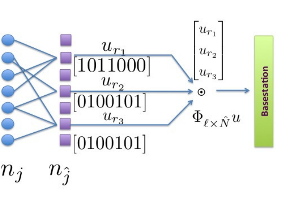
We design a distributed algorithm for EAST+where nodes locally generate projections without communicating with base and thus save the additional energy required by the centralized approach for base to node communication. Our description so far has assumed , however EAST+can be readily extended to the case with . In this case, we consider the sensor measurement collected at time () by sensor (). We will also vectorize the 2-dimensional signal . We will abuse the notation and use to denote this vector (this should be clear from the context). The vector has elements where the -th element of is where . The corresponding projection matrix is now an matrix. For , the elements in the -th column of the projection matrix ( with ) are generated by Equation (4) with parameter and these elements will determine whether the sensor will sample at time . We will now describe an algorithm which is used by EAST+to recover an approximation of the signal (), from the sparse projections created locally in different nodes.
- •
First each node () generates the random numbers using the distribution function mentioned in Equation (4). Each of is responsible for generating the -th row () of the projection matrix. Consider the element in the projection matrix and let us assume that the column index and the node-time pair have one-to-one correspondence given by .
- •
If , node asigns node to sample at time and node sends the sample to node .
- •
Upon receiving from node , computes (where ). Node performs this operation for all the values it receives and finally transmits to the base station. This process is repeated for all node
- •
After receiving transmissions from the nodes, base station has . It then generates using the same seed as the nodes. Finally, with , and , base station uses low-complexity sketching decoder to recover the signal. The complexity of the decoder is .
V Experimental Results
In this Section we use the data collected from energy hungry wind speed and wind direction sensors at the Springbrook deployment to evaluate the performance of EAST+.
V-A Experimental Setup
Let be the approximation of the signal , we use relative error, to determine the accuracy of the approximation. The relative error is a commonly used error metric in the signal processing literature [17, 16] that tells us how close the approximate signal is to the real signal.
We used data from of the sensing nodes from Springbrook National Park deployment. Amongst these nodes (shown in Figure 4), node is deep in the forest whereas the rest of the nodes are in the open space. Consequently, the solar current harvest rate of node is the lowest whereas the rest of the nodes have higher (also similar) harvest rates. Inter-sampling interval in the deployment is minute. We collected one month of data which gave us snapshots of both wind speed and wind direction sensor data. Note that sketching decoder computes the estimation from median, therefore, it performs better approximation with large . We used , by segmenting our snapshots from nodes into group of each. Below we define a number of variants of EAST+that we will use in the results.

EAST+-Upperbound: Given the energy profile of the nodes, we solve the optimization problem in (18) to determine this minimum value of the upper bound of the approximation error. We call this error EAST+-Upperbound. We use the Matlab optimization solver “fmincon” to solve (18).
EAST+-Empirical: The difference between this and EAST+-Upperbound is that, unlike EAST+-Upperbound, the error is not given by the solution of (18). The error is calculated from the reconstruction of the real data, such as wind speed and wind direction data. However, for various data length , we use the optimal and given by EAST+-Upperbound.
EAST-Equality: EAST+uses inequality constraints and we conjecture that the optimal solution given by EAST+requires only one constraint to be active. Precisely, we conjecture that the optimal solution requires only the node with minimum energy to operate at “exact” energy neutral operation. Let us now envision another solution where all the constraints are active, i.e.
| (19) |
We will refer to this variant as EAST-Equality.
V-B Results


In the results section we first verify whether the wind data satisfy the bounded peak-to-total energy condition. In Figure 5 we plot the peak to total energy ratio for various . We observe that for both of the wind sensor data, is bounded by and . This satisfies the peak-to-total energy condition.
We report the performance of EAST+in Figure 6. In general, the approximation error decreases as the length of the signal () increases. This can be explained using the behavior of sketching decoder, which performs better when the length of the signal is large. Clearly, EAST+-Upperbound provides the upper bound of the reconstruction error for all the values of . It provides the upper bound for EAST, EAST+-Empirical and EAST-Equality.
We also compare the performance of EAST+with our previously proposed EAST. In particular, we compare EAST+-Empirical with EAST. We choose sufficiently large values of and for EAST, which ensure energy neutral operations. In Table I we report three sets of and used for wind direction. Similar values of and were chosen for wind speed. The three reconstructions using these three set of values are referred to as EAST-1, EAST-2 and EAST-3 in Figure 6. We find that EAST+-Empirical achieves significant error reduction compared to EAST-1, EAST-2 and EAST-3. The error reduction is highest when signal length is small. For example, for wind speed, when signal length is 64, the error reduction is approximately 17% compared to the EAST-1 (We compare with EAST-1, since it performs better than EAST-2 and EAST-3). Similarly, for wind direction, the error reduction is approximately 30%. However, the error reduction diminishes as the length of the signal increases. For wind speed the error reduction is 8% when signal length is 2048. Note that for in-situ signal processing on resource improvised sensor nodes, small signal length is desirable. Therefore, EAST+is highly preferable over EAST for wireless sensor networks.
Finally, we compare EAST+-Emperical with EAST-Equality. The comparison results show that these two have similar reconstruction performances. In East-Equality all the nodes operate at exact energy neutral condition. Therefore, East-Equality would require higher sampling energy compared to EAST+. However, despite sampling at a higher rate, East-Equality does not offer any significant reconstruction improvement compared to EAST+-Empirical. This further substantiates our claim that EAST+is optimal.
| =64 | =128 | =256 | =512 | =1024 | =2048 | |||||||||||||||||||
| E1 | E2 | E3 | E1 | E2 | E3 | E1 | E2 | E3 | E1 | E2 | E3 | E1 | E2 | E3 | E1 | E2 | E3 | |||||||
| 413 | 290 | 370 | 368 | 850 | 660 | 720 | 740 | 1500 | 1290 | 1460 | 1482 | 3295 | 2675 | 2950 | 2968 | 6370 | 5150 | 5910 | 5940 | 12200 | 11190 | 11780 | 11883 | |
| 0.06 | 0.1 | 0.08 | 0.0945 | 0.01 | 0.05 | 0.02 | 0.0473 | 0.009 | 0.03 | 0.0239 | 0.0236 | 0.009 | 0.02 | 0.008 | 0.0118 | 0.0023 | 0.0071 | 0.0047 | 0.0059 | 0.0013 | 0.0047 | 0.0021 | 0.0030 | |
VI Related Work
Energy conservation in wireless sensor networks is a heavily studied field. Below we rationalize the uniqueness of EAST+with respect to the related literature. In [18] an adaptive sampling algorithm is presented which can be used for estimating the best sampling frequency for energy hungry sensors. However, their approach assumes that the sensors have uniform energy profiles.
Work presented in [19] proposes a harvest-aware adaptive sampling approach to dynamically identify the maximum duty cycle. However, their focus is not on signal approximation from the network.
In [20], a Bayesian estimation technique is presented to estimate the wind speed and wind direction signals. The authors have supplemented their estimation using the assumption that the wind speed and wind direction signals have a correlation with hourly tide data. However, in our work we assume that signals are compressible due to the presence of spatial-temporal correlation among the data collected at different sensing nodes.
A number of studies [21, 22, 23] have utilized the spatial-temporal correlation of the signal to reduce sampling requirements. Though our approach has similar assumption, we have considered non-uniform energy profile of the sensors, which is different. Moreover, we have used Sparse Random Projections, which is also different from these approaches.
A large number of signal approximation techniques use Compressive Sensing [24, 12] to conserve transmission energy assuming that radio is the dominant component of energy consumption, however we assume energy-hungry sensor dominates the energy consumption. A slightly different compressive sensing based data gathering approach is presented in [25] which investigates the impact of a routing topology generated sparse projection matrix on the accuracy of the approximation. Our work is different from theirs since our projection matrix is not based on the routing topology rather it is populated based on the energy profile of the sensors. A more general sparse projection matrix proposed in the compressive sensing literature can be found in [26]. However, the non-zero elements of this sparse projection matrix are chosen uniform randomly, but, in order to enable energy-aware sampling, the non-zero elements in the projection matrix need to be chosen nonuniform randomly.
Recently, we have extended the theory of compressive sensing showing that it can be used to support non-uniform sampling [27, 28]. However, in this paper we choose sparse random projections over compressive sensing, since the decoding process of compressive sensing is computationally expensive. The complexity of decoding a data point vector is . Whereas, decoding complexity of sparse random projections is as low as , where is the number of projections. In this paper the projects are generated locally without any coordination between basestation and nodes, and, the final signal recovery takes place at the resource enriched basestation. In our future study we seek to conduct the signal recovery at the resource limited sensor nodes. For that purpose a low complexity decoder will be very useful.
VII Conclusion
In this paper we propose EAST+, which offers an optimal sensing strategy for any rechargeable wireless sensor networks with energy hungry sensors. We derive the upper bound of reconstruction error for EAST+. Then using two energy hungry sensor (wind speed and wind direction sensor) data from Springbrook National park sensor deployment, we evaluate the validity of the upper bound of the reconstruction error. We compare EAST+with our previously proposed signal reconstruction method EAST. The shortcoming of EAST is that it does not guarantee the optimal utilization of node energy, which could potentially compromise reconstruction accuracy. The comparison results presented in this paper clearly show that EAST+can significantly reduce the reconstruction error. We also present a distributed algorithm for EAST+, which can be readily used in the sensor network deployments. In our future study we want to study the adaptation of dynamic change in energy profile.
References
- [1] GDI, “Habitat monitoring on great duck island. http://www.greatduckisland.net/index.php,” 2002.
- [2] T. Wark, W. Hu, P. Corke, J. Hodge, A. Keto, B. Mackey, G. Foley, P. Sikka, and M. Brünig., “Springbrook: Challenges in developing a long-term rainforest wireless sensor network,” in Proceeding of The International Conference on Intelligent Sensors, Sensor Networks and Information Processing (ISSNIP), Sydney, Australia, Dec 2008.
- [3] G. Anastasi, M. Conti, M. Francesco, and A. Passarella, “Energy conservation in wireless sensor networks: A survey,” Ad Hoc Networks, vol. 7, no. 3, pp. 537–568, May 2009. [Online]. Available: http://dx.doi.org/10.1016/j.adhoc.2008.06.003
- [4] W. Hu, N. Bulusu, C. T. Chou, S. Jha, A. Taylor, and V. N. Tran, “Design and evaluation of a hybrid sensor network for cane toad monitoring,” ACM Transactions on Sensor Network, vol. 5, no. 1, pp. 1–28, 2009.
- [5] M. Zhao, J. Li, and Y. Yang, “Joint mobile energy replenishment and data gathering in wireless rechargeable sensor networks,” in Proceedings of the 23rd International Teletraffic Congress. International Teletraffic Congress, 2011, pp. 238–245.
- [6] L. Yerva, B. Campbell, A. Bansal, T. Schmid, and P. Dutta, “Grafting energy-harvesting leaves onto the sensornet tree,” in Proceedings of the 11th international conference on Information Processing in Sensor Networks. ACM, 2012, pp. 197–208.
- [7] V. Raghunathan, A. Kansal, J. Hsu, J. Friedman, and M. Srivastava, “Design considerations for solar energy harvesting wireless embedded systems,” in IPSN ’05: Proceedings of the 4th international symposium on Information processing in sensor networks. Los Angeles, California: IEEE Press, 2005, p. 64.
- [8] W. Bajwa, J. Haupt, A. Sayeed, and R. Nowak, “Compressive wireless sensing,” in IPSN ’06: Proceedings of the fifth international conference on Information processing in sensor networks, Nashville, Tennessee, USA, 2006, pp. 134–142.
- [9] S. Sivapalan, R. K. Rana, D. Chen, S. Sridharan, S. Denmon, and C. Fookes, “Compressive sensing for gait recognition,” in Digital Image Computing Techniques and Applications (DICTA), 2011 International Conference on. IEEE, 2011, pp. 567–571.
- [10] J. Xu, S. Denman, S. Sridharan, C. Fookes, and R. Rana, “Dynamic texture reconstruction from sparse codes for unusual event detection in crowded scenes,” in Proceedings of the 2011 joint ACM workshop on Modeling and representing events. ACM, 2011, pp. 25–30.
- [11] S. W. Chew, R. Rana, P. Lucey, S. Lucey, and S. Sridharan, “Sparse temporal representations for facial expression recognition,” in Advances in Image and Video Technology. Springer, 2012, pp. 311–322.
- [12] R. Rana, W. Hu, T. Wark, and C. T. Chou, “An adaptive algorithm for compressive approximation of trajectory (aacat) for delay tolerant networks,” in Wireless Sensor Networks. Springer, 2011, pp. 33–48.
- [13] B. Wei, M. Yang, R. K. Rana, C. T. Chou, and W. Hu, “Distributed sparse approximation for frog sound classification,” in Proceedings of the 11th international conference on Information Processing in Sensor Networks. ACM, 2012, pp. 105–106.
- [14] R. Rana, W. Hu, and C. T. Chou, “Energy-aware sparse approximation technique (east) for rechargeable wireless sensor networks,” in Wireless Sensor Networks. Springer, 2010, pp. 306–321.
- [15] E. J. Candes and J. Romberg, “Practical signal recovery from random projections,” in Proc. SPIE Computational Imaging, vol. 5674, San Jose, 2005, pp. 76–86.
- [16] W. Wang, M. Garofalakis, and K. Ramchandran, “Distributed sparse random projections for refinable approximation,” in IPSN ’07: Proceedings of the 6th international conference on Information processing in sensor networks, Cambridge, Massachusetts, USA, 2007, pp. 331–339.
- [17] S. Ji, Y. Xue, and L. Carin, “Bayesian compressive sensing,” IEEE Transaction on Signal Processing, vol. 56, no. 6, pp. 2346–2356, 2008.
- [18] C.Alippi, G. Anastasi, M. D. Francesco, and M. Roveri, “An adaptive sampling algorithm for effective energy management in wireless sensor networks with energy-hungry sensors,” IEEE-Transactions on Instrumentation and Measurement, vol. 58, no. 11, pp. 335–344, Nov 2009.
- [19] A. Kansal, J. Hsu, S. Zahedi, and M. B. Srivastava, “Power management in energy harvesting sensor networks,” Trans. on Embedded Computing Sys., vol. 6, no. 4, p. 32, 2007. [Online]. Available: http://dx.doi.org/10.1145/1274858.1274870
- [20] S. Reboul and M. Benjelloun, “Joint segmentation of the wind speed and direction,” Signal Process, vol. 86, no. 4, pp. 744–759, 2006.
- [21] C. Liu, K. Wu, and J. Pei, “An energy-efficient data collection framework for wireless sensor networks by exploiting spatiotemporal correlation,” IEEE Transactions on Parallel Distributed Systems, vol. 18, no. 7, pp. 1010–1023, 2007.
- [22] R. Willett, A. Martin, and R. Nowak, “Backcasting: adaptive sampling for sensor networks,” in IPSN ’04: Proceedings of the 3rd international symposium on Information processing in sensor networks, Berkeley, California, USA, 2004, pp. 124–133.
- [23] H. Gupta, V. Navda, S. Das, and V. Chowdhary, “Efficient gathering of correlated data in sensor networks,” ACM Transactions Sensor Networks, vol. 4, no. 1, pp. 1–31, 2008.
- [24] Duarte et al., “Universal distributed sensing via random projections,” in IPSN ’06: Proceedings of the 5th international conference on Information processing in sensor networks. Nashville, Tennessee, USA: ACM, 2006, pp. 177–185.
- [25] G. Quer et al., “On the interplay between routing and signal representation for compressive sensing in wireless sensor networks,” San Diego, USA, JAN 2007.
- [26] R. Baraniuk, M. Davenport, R. DeVore, and M. Wakin, “A Simple Proof of the Restricted Isometry Property for Random Matrices,” Constructive Approximation, vol. 28, no. 3, pp. 253–263, July 2006. [Online]. Available: http://dx.doi.org/10.1134/S0021364006090037
- [27] Y. Shen, W. Hu, R. Rana, and C. T. Chou, “Non-uniform compressive sensing in wireless sensor networks: Feasibility and application,” in Intelligent Sensors, Sensor Networks and Information Processing (ISSNIP), 2011 Seventh International Conference on, Dec 2011, pp. 271–276.
- [28] Y. Shen, W. Hu, R. Rana, and C. T. Chou, “Nonuniform compressive sensing for heterogeneous wireless sensor networks,” IEEE Sensors, vol. 13, no. 6, pp. 2120–2128, 2013.
APPENDIX
Proof VII.1 (Proof of Proposition III.1)
It can be proved that the projection matrix defined by Equation (4) satisfies these conditions:
| (20) |
Define independent random variables where, Expectation and second moment of can be computed as,
Since , using the above result we can show that:
In order to prove proposition III.2, we need the following lemma.
Lemma VII.2
Consider a data vector which satisfies condition (). Let . Consider a sparse random matrix satisfies condition (20), with sparsity parameter . Define . The random projections and then produces an estimation for , with probability at least , satisfying ,
Proof VII.3 (Proof of Lemma VII.2)
Consider two vectors that satisfies condition (). Set where and are two positive integers. Partition the matrix into matrices each of size . Create the random projections and
Let us define the independent random variables , where . We now apply Proposition III.1 to each and find that, and
Using Chebyshev inequality it can be shown that,
Therefore, we can obtain a constant probability by setting .
Therefore, we can obtain a constant probability, say , by setting .
Now it can be shown that [16] for any pair of vectors and , the random projections and produce an estimate for that lies outside the tolerable approximation interval with probability at most , where is some constant. Taking union bound over all such vectors, the probability that at least one lies outside the tolerable interval with probability is upper bounded by
Now,
Proof VII.4 (Proof of Proposition III.2)
Consider an orthonormal transform . Let us represent the transform coefficients using . Reordering the transform coefficients in decreasing of magnitude, i.e., , the approximation error by taking the largest coefficients in magnitude, and setting the remaining coefficients to zero is given by . Let and assume that satisfies condition (), with positive integer, The random projections and can produce estimates , where the estimates satisfy with high probability (Lemma VII.2).
It can be shown that [16] for , the approximate error is: Therefore the number of random projections can be given by