We revisit the transformation rules of the metric and Kalb-Ramond field under T-duality, and express the corresponding relations in terms of the metric $G$ and the field strength $H=dB$ . In the course of the derivation, we find an explanation for potential reductions of the isometry group in the dual background.

The formalism employed in this paper is illustrated with examples based on tori and spheres, where for the latter we construct a new non-geometric background.

1 Introduction

One of the intriguing features of string theory is that it comprises a rich structure of dualities. Amongst them is target-space duality, or T-duality in short, which in its simplest form states that string theory compactified on a circle of radius $R$ is equivalent to a compactification on a circle with radius $\alpha^{\prime}/R$ (see [1] and the references therein). For the circle, the duality group is given by $\mathbb{Z}_{2}$ , but for toroidal backgrounds one finds that it takes the form $O(d,d,\mathbb{Z})$ where $d$ denotes the number of compact dimensions. Other dualities for string theory are $S$ -duality, which is a strong-weak duality, the combination of it with T-duality into so-called $U$ -duality, and also the AdS/CFT duality. However, in this work we are primarily interested in T-duality.

Dualities have played an important role in understanding the structure of string theory and in uncovering new features; a prominent example thereof is the discovery of D-branes. More recently, T-duality has helped to find new solutions of the theory with surprising and unusual properties. In particular, it turns out that not only ordinary geometric spaces are eligible backgrounds for string theory, but that so-called non-geometric configurations with non-commutative and even non-associative features are possible as well. The latter have been found by applying successive T-duality transformations to a three-torus with non-vanishing field strength $H=dB$ for the Kalb-Ramond field $B$ , which we are going to review briefly in the following.

•

Starting from a flat three-torus with non-trivial flux $H$ , one performs a T-duality transformation along a direction of isometry. This results in a twisted torus [2, 3] with vanishing field strength, where the topology is characterized by a so-called geometric flux $f$ [4, 5].
•

For the twisted torus, an additional T-duality transformation can be performed. The resulting background allows for a locally-geometric description, but is globally non-geometric [6]. The latter means that when considering a covering of the torus by open neighborhoods, the transition functions on the overlap of these charts are not solely given by diffeomorphisms, and hence such a manifold cannot be described by Riemannian geometry. However, if in addition to diffeomorphisms one considers T-duality transformations as transition maps [7], this space can be globally defined. This construction is usually called a T-fold [8], and carries a so-called $Q$ -flux [9].

Note that the $Q$ -flux is related to non-commutative features of this background, which have been studied in a variety of publications [10, 11, 12, 13, 14, 15, 16, 17, 18].
•

Finally, for the T-fold it has been argued that one can formally perform a third T-duality transformation [9]. Here it has been found that the resulting $R$ -flux background is not even locally geometric, and that it carries a non-associative structure.

These backgrounds have first been studied from a mathematical point of view in [19, 20], later in [21], and have recently been reconsidered in a series of papers [22, 23, 24, 14, 25, 26, 16, 18].

The chain of T-duality transformations reviewed here is usually summarized by illustrating how the fluxes in the various backgrounds are related. One finds the following schematic picture [9]

\begin{split}H_{xyz}\quad\xleftrightarrow{\;\;\;T_{z}\;\;\;}\quad f_{xy}{}^{z}\quad\xleftrightarrow{\;\;\;T_{y}\;\;\;}\quad Q_{x}{}^{yz}\quad\xleftrightarrow{\;\;\;T_{x}\;\;\;}\quad R^{xyz}\;.\end{split}

(1.1)

However, let us remark that non-geometric backgrounds can not only be obtained by a chain of T-duality transformations similar to (1.1), but can also be realized in the context of asymmetric orbifolds. Examples for such constructions can be found for instance in [7, 6, 27, 28, 29, 23, 15, 30].

Non-geometric flux backgrounds, in particular the T-fold background mentioned above, have been investigated in a number of publications over the years. We do not want to mention all the corresponding references here, but only touch upon a few topics. For one, there are the papers by Hull and collaborators where non-geometric flux configurations have been studied from a doubled-geometry point of view [8, 31, 32]. More recently, non-geometric backgrounds have been investigated via field redefinitions for the ten-dimensional supergravity action in [33, 34, 35, 36, 37, 38, 39]. However, as was found in [38], such methods do not allow for a global description of non-geometric flux backgrounds. Let us also mention that a discussion of non-geometric backgrounds from a world-sheet point of view can be found in [28, 40, 41], and for studies in the context of double-field theory we would like to refer the reader to the reviews [42, 43].

The main motivation for the present paper is that almost all examples for non-geometric flux backgrounds are constructed by applying T-duality transformations to tori. Compared to the landscape of string-theory solutions, this is a very restricted family of configurations. In addition, it should be noted that, strictly speaking, toroidal backgrounds with fluxes (and constant dilaton) do not solve the string-equations of motion. Therefore, one should go beyond the family of tori and search for new examples of non-geometric spaces.

A well-studied class of proper string-theory backgrounds with non-trivial $H$ -flux is given by Wess-Zumino-Witten models [44, 45], which describe strings moving on group manifolds. One of the simplest examples thereof is based on the group $SU(2)$ and corresponds to $S^{3}$ with a non-vanishing flux $H$ . For such a background, T-duality has been studied for instance in [46], where the authors found that the dual space is given by a circle bundle over $S^{2}$ . However, no indications of a non-geometric structure have been observed. In the present paper, we consider a slightly modified setting and investigate $S^{3}\times S^{1}$ together with a particular choice of $H$ -flux. As we describe in detail, after applying two T-duality transformations to this space, we arrive at a background which is a non-geometric T-fold, and which therefore provides a second class of examples for studying non-geometry.

In the remainder of this paper, we first review the sigma-model action for the closed string in section 2. We study its symmetry structure and find that it can be described in terms of the so-called $H$ -twisted Courant bracket. In section 3, we follow Buscher’s procedure [47, 48, 49] and gauge a symmetry of the closed-string sigma-model action. Upon integrating out the gauge field, we obtain a formulation describing the T-dual background. However, in contrast to the Buscher rules which are expressed in terms of the metric $G$ and the Kalb-Ramond field $B$ , here we derive formulas for $G$ and $H=dB$ . The advantage of this formalism is that no ambiguity in choosing a gauge for the initial configuration arises. In section 4 we illustrate this method, and discuss T-duality transformations for tori. Due to the formulation in terms of the field strength, we are able to obtain generalizations of the examples known in the literature. In section 5 we turn to configurations based on spheres, where we first review and generalize the known results for the three-sphere, and subsequently present a new example of a non-geometric background. Finally, in section 6, we close with a summary and conclusion.

2 Sigma-model action for the closed string

We begin our discussion of T-duality transformations by reviewing the sigma-model action for the closed string. This action encodes the dynamics of a target-space metric $G$ , an anti-symmetric Kalb-Ramond field $B$ and a dilaton $\phi$ , and is usually defined on a compact two-dimensional world-sheet without boundaries. However, when considering non-trivial field strengths $H=dB\neq 0$ , one should employ the Wess-Zumino term for the Kalb-Ramond field in order to have a globally well-defined description on the target space.

Action

Since here we are indeed interested in configurations with $H\neq 0$ , we formulate the action in the following way. Denoting by $\Sigma$ a three-dimensional Euclidean manifold with compact boundary $\partial\Sigma$ , we have

\begin{split}\mathcal{S}=&-\frac{1}{4\pi\alpha^{\prime}}\int_{\partial\Sigma}\Bigl[G_{ij}\,dX^{i}\wedge\star dX^{j}+\alpha^{\prime}R\,\phi\star 1\Bigr]\\[5.69054pt] &-\frac{i}{2\pi\alpha^{\prime}}\int_{\Sigma}\tfrac{1}{3!}\,H_{ijk}\hskip 1.0ptdX^{i}\wedge dX^{j}\wedge dX^{k}\,.\end{split}

(2.1)

The Hodge-star operator $\star$ is defined on the two-dimensional world-sheet $\partial\Sigma$ , and the differential is understood as $dX^{i}(\sigma^{\mu})=\partial_{\mu}X^{i}d\sigma^{\mu}$ with $\{\sigma^{\mu}\}$ coordinates on $\partial\Sigma$ and on $\Sigma$ . The indices $i,j$ take values $i,j\in\{1,\ldots,d\}$ with $d$ the dimension of the target space, and $R$ denotes the curvature scalar corresponding to the metric on $\partial\Sigma$ .

Note that the choice of a three-manifold $\Sigma$ for a given boundary $\partial\Sigma$ is not unique. But, if the (expectation value of the) field strength $H$ is quantized, then the path integral only depends on the data of the two-dimensional theory [50]. In our conventions, the quantization condition reads

\begin{split}\frac{1}{2\pi\alpha^{\prime}}\int_{\Sigma}H\;\in\;2\pi\hskip 1.0pt\mathbb{Z}\,.\end{split}

(2.2)

Coming to a slightly more technical point, in the following we require the world-sheet fields $X^{i}$ appearing in the action (2.1) – and therefore also $G_{ij}(X)$ , $\phi(X)$ and $H_{ijk}(X)$ – to be well-defined on $\Sigma$ and $\partial\Sigma$ . More concretely, in order to apply Stoke’s theorem in our computations below, the scalars $X^{i}$ should be single-valued as world-sheet fields. This means that we ignore contributions from winding and momentum modes, and hence work in a supergravity approximation.¹¹ 1 Of course, if the metric, field strength and dilaton do not depend on $X^{i}$ , only the differentials $dX^{i}$ appear in the action (2.1) and hence winding and momentum modes can be incorporated. Furthermore, we study the sigma-model action (2.1) at the classical level, and therefore do not take into account restrictions coming for instance from the vanishing of the conformal anomaly.

Invariance under field redefinitions

In addition to the usual world-sheet symmetries, the action (2.1) can be invariant under field redefinitions of the target-space coordinates $X^{i}$ . Let us therefore consider the following change of coordinates for a constant parameter $\epsilon$

\begin{split}\delta_{\epsilon}X^{i}=\epsilon\hskip 1.0ptk^{i}(X)\,.\end{split}

(2.3)

Under this variation, the action (2.1) changes as

\begin{split}\delta_{\epsilon}\hskip 1.0pt\mathcal{S}=&-\frac{1}{4\pi\alpha^{\prime}}\int_{\partial\Sigma}\,\epsilon\hskip 1.0pt\Bigl[\,\mathcal{L}_{k}G+\alpha^{\prime}R\bigl(\mathcal{L}_{k}\phi\bigr)\star 1\,\Bigr]-\frac{i}{2\pi\alpha^{\prime}}\int_{\Sigma}\epsilon\,\mathcal{L}_{k}H\,,\end{split}

(2.4)

where $\mathcal{L}_{k}=d\circ\iota_{k}+\iota_{k}\circ d$ denotes the Lie derivative in the direction of the vector $k$ , and $\iota_{k}$ is the insertion map. The variation of the action (2.4) vanishes if three conditions are met. First, $k$ is a Killing vector of the target-space metric $G$ , i.e.

\begin{split}\mathcal{L}_{k}\hskip 1.0ptG=0\,,\end{split}

(2.5)

where we employ the coordinate-free notation $G=G_{ij}\hskip 1.0ptdX^{i}\wedge\star dX^{j}$ . Second, the term involving $\mathcal{L}_{k}H$ vanishes, which can be expressed as

\begin{split}\iota_{k}H=dv\,,\end{split}

(2.6)

for $v$ a one-form on the target space [51, 52] (see also [53]). Note that $v$ in (2.6) is defined only up to a closed part. Finally, the third condition for the variation (2.4) to vanish is that

\begin{split}\mathcal{L}_{k}\phi=k^{i}\partial_{i}\phi=0\,.\end{split}

(2.7)

Algebraic structure of field redefinitions

Let us now investigate a situation in which the metric $G$ has several Killing vectors. From the commutator property of the Lie derivative it follows that if $k_{(1)}$ and $k_{(2)}$ are Killing vectors, also the Lie bracket $k_{(3)}=[k_{(1)},k_{(2)}]_{\rm L}$ is a Killing vector

\begin{split}\mathcal{L}_{k_{(3)}}G=\mathcal{L}_{[k_{(1)},k_{(2)}]_{\rm L}}\hskip 1.0ptG=0\,.\end{split}

(2.8)

This can alternatively be inferred from the closure of the algebra generated by (2.3). A similar analysis can be applied to the condition (2.6). Up to exact terms, we find that the one-form $v_{(3)}$ corresponding to the Killing vector $k_{(3)}$ is given by

\begin{split}v_{(3)}=\tfrac{1}{2}\left(\mathcal{L}_{k_{(1)}}v_{(2)}-\mathcal{L}_{k_{(2)}}v_{(1)}\right).\end{split}

(2.9)

The structure describing the algebra of field redefinitions (2.3) which leave the action (2.1) invariant can then be formulated using the so-called $H$ -twisted Courant bracket [54]. The latter is defined as follows

		$\displaystyle\bigl[k_{(1)}+v_{(1)},k_{(2)}+v_{(2)}\bigr]^{H}_{\rm C}$
		$\displaystyle\hskip 30.0pt=\bigl[k_{(1)},k_{(2)}\bigr]_{\rm L}+\mathcal{L}_{k_{(1)}}v_{(2)}-\mathcal{L}_{k_{(2)}}v_{(1)}-\tfrac{1}{2}\,d\bigl(\iota_{k_{(1)}}v_{(2)}-\iota_{k_{(2)}}v_{(1)}\bigr)-\iota_{k_{(1)}}\iota_{k_{(2)}}H$
		$\displaystyle\hskip 30.0pt=k_{(3)}+v_{(3)}\,,$		(2.10)

where the formal sum of a vector and a one-form is considered as an element of the generalized tangent space $TM\oplus T^{*}M$ , with $M$ the target-space manifold.²² 2 For more details on generalized geometry we would like to refer the reader to the original papers [55] and [56], and for instance to [57] for a less mathematical discussion. Let us make the following remarks:

•

The one-forms $v_{(a)}$ in equation (2.6) are defined only up to terms which are closed, and hence also the Courant bracket (2.10) is defined only up to closed expressions. This, in turn, leaves some freedom to express the algebraic structure of field redefinitions; for different formulations and further details see for instance [58].
•

The automorphisms of the Courant bracket [56] are given by diffeomorphisms of the target-space coordinates, and by transformations involving a closed two-form $\Omega$ .³³ 3 The $\Omega$ -transform introduced here is usually called a $B$ -transform. But in order to avoid confusion with the Kalb-Ramond field introduced above, we employ the notation $\Omega$ . This is also true for the $H$ -twisted Courant bracket (2.10), and the explicit form of the $\Omega$ -transform reads

$\begin{split}k+v\;\to\;k+(v+\iota_{k}\Omega)\hskip 30.0pt\mbox{for}\hskip 30.0ptd\Omega=0\,.\end{split}$ (2.11)
•

It is known that for the untwisted Courant bracket, in general the Jacobi identity is not satisfied [56]. In particular, the Jacobiator

$\begin{split}{\rm Jac}(A,B,C)_{\rm C}=\bigl[A,[B,C]_{\rm C}\bigr]_{\rm C}+{\rm cyclic}\end{split}$ (2.12)

is equal to an exact term. In the present context, this does not pose a problem since the bracket (2.10) is defined only up to closed expressions (see also [58], especially sections 6 and 7). For the $H$ -twisted Courant bracket the situation is analogous, provided that $H$ satisfies the Bianchi identity $dH=0$ [56].
•

As we have shown here, the $H$ -twisted Courant bracket (2.10) originates naturally from the global symmetry structure of the sigma model (2.1). The untwisted Courant bracket appears in the framework of ordinary generalized geometry and is well-studied, however, to our knowledge an $H$ -twisted version of generalized geometry has only been investigated in detail in the mathematical literature [59]. But, it would be interesting to apply the $H$ -twisted formalism to questions in a physical context.

3 T-duality

We now turn to our discussion of T-duality and review the transformation rules for the metric, Kalb-Ramond field and dilaton. These rules can be derived by gauging a target-space isometry in a corresponding sigma model [47, 48, 49], which in addition to the original papers has been discussed in a variety of publications in the past. The work which is of particular relevance for our approach here can be found in [51, 60, 52, 61, 62, 63].

3.1 Gauging a symmetry

Let us start by gauging the symmetry (2.3) of the action (2.1). In the literature, slightly different ways of obtaining a gauged action can be found; here we follow the procedure explained in [62], which is less restrictive than the formalism discussed for instance in [51, 52].

The gauged action

We gauge an isometry of the target-space metric by allowing $\epsilon$ in (2.3) to have a non-trivial dependence on the world-sheet coordinates. This implies that we have to introduce a gauge field $A$ and replace $dX^{i}\to dX^{i}+k^{i}A$ for the term involving the metric. For the Wess-Zumino term we keep $dX^{i}$ unchanged, but introduce an additional scalar field $\chi$ . The resulting gauge-invariant action then takes the following form

	$\displaystyle\widehat{\mathcal{S}}=$	$\displaystyle-\frac{1}{4\pi\alpha^{\prime}}\int_{\partial\Sigma}\Bigl[G_{ij}(dX^{i}+k^{i}A)\wedge\star(dX^{j}+k^{j}A)+2\hskip 1.0pti(v+d\chi)\wedge A+\alpha^{\prime}R\,\phi\star 1\Bigr]$
		$\displaystyle-\frac{i}{2\pi\alpha^{\prime}}\int_{\Sigma}\tfrac{1}{3!}\,H_{ijk}\hskip 1.0ptdX^{i}\wedge dX^{j}\wedge dX^{k}\,,$		(3.1)

where $k$ denotes the Killing vector of the target-space isometry which has been gauged. The explicit form of the symmetry transformations for the fields in the action reads

\begin{split}\hat{\delta}_{\epsilon}X^{i}=\epsilon\hskip 1.0ptk^{i}(X)\,,\hskip 50.0pt\hat{\delta}_{\epsilon}A=-d\hskip 1.0pt\epsilon\,,\hskip 50.0pt\hat{\delta}_{\epsilon}\chi=-\epsilon\hskip 1.0ptk^{i}v_{i}\,,\end{split}

(3.2)

and the corresponding variation of (3.1) becomes

\begin{split}\hat{\delta}_{\epsilon}\hskip 1.0pt\widehat{\mathcal{S}}=\frac{i}{2\pi\alpha^{\prime}}\int_{\partial\Sigma}d\chi\wedge d\epsilon\,,\end{split}

(3.3)

which at this point is non-vanishing. As mentioned below equation (2.2), in the above computations we have assumed the fields $X^{i}$ to be single valued on the world-sheet. However, there can be large gauge transformations if the two-dimensional world-sheet $\partial\Sigma$ is compact and hence $\epsilon$ can be multivalued [62]. Denoting then by $\gamma$ a non-trivial one-cycle of $\partial\Sigma$ and by $\ell_{\rm s}=2\pi\sqrt{\alpha^{\prime}}$ the string length, we can normalize

\begin{split}\int_{\gamma}d\epsilon\;\in\;\ell_{\rm s}\hskip 1.0pt\mathbb{Z}\,.\end{split}

(3.4)

Coming back to (3.3), this variation vanishes in the path integral if $\delta_{\epsilon}\hskip 1.0pt\widehat{\mathcal{S}}$ is a multiple of $2\pi\hskip 1.0pti$ . Therefore, taking into account (3.4), the scalar field $\chi$ should be periodic on the world-sheet $\partial\Sigma$ with period determined by

\begin{split}\int_{\gamma}d\chi\;\in\;\ell_{\rm s}\hskip 1.0pt\mathbb{Z}\,.\end{split}

(3.5)

Remarks

After having shown the gauged action (3.1) to be invariant under the transformations (3.2), let us make the following three remarks.

•

The equations of motion for the scalar field $\chi$ imply that the field strength $F=dA$ has to vanish. Recalling then from (3.5) that $\chi$ can be multivalued, one can argue that in the path integral the term $d\chi\wedge A$ produces a delta-function which sets to zero the holonomy of the gauge field [61]. This implies that $A$ is pure gauge on the world-sheet $\partial\Sigma$ .
•

Note that the ungauged action (2.1) is expressed in terms of the metric tensor, the dilaton and the field strength $H$ , which are globally defined on the target space.⁴⁴ 4 Let us mention that we call an object globally defined if it corresponds to a single-valued tensor field on the target-space manifold. When gauging this action, we implicitly assumed that the Killing vector $k$ is a global object. But, in (3.1) also the one-form $v$ appears, which in general is only locally defined. Hence, a priori the gauged action (3.1) is valid only locally on the target space.

Figure 1: Illustration of the local structure of the gauged world-sheet action (3.1) on the target space $M$ . The action depending on $v_{1}$ is valid in the first patch of $M$ , while the action depending on $v_{2}$ is valid in the second patch. On the overlap, the actions agree provided there exists a function $\Lambda_{12}$ such that $v_{1}-v_{2}=d\Lambda_{12}$ .

However, recall that $v$ is defined up to closed terms, and denote by $v_{1,2}$ the one-form in two different charts. If on the overlap of these charts there exists a function $\Lambda_{12}$ such that $v_{1}-v_{2}=d\Lambda_{12}$ , one can define $v$ , and henceforth the world-sheet action (3.1), properly on the whole target space. This is illustrated in figure 1, and has been discussed in detail in [64].
•

Note that the assumption of a globally-defined Killing vector $k$ is not always satisfied. In this situation, the gauged action (3.1) is valid only locally on the target space. This question has also been discussed in [64], and we come back to this point in sections 4.2 and 5.2.

Multiple global symmetries

Let us now study the situation where the action (2.1) possesses multiple global symmetries, out of which one has been gauged. The Killing vector corresponding to the gauged symmetry is denoted by $k$ , and Killing vectors for the global symmetries are denoted by $Z$ . We now want to ask the question under what conditions the action (3.1) is invariant under the remaining global symmetries

\begin{split}\tilde{\delta}_{\tilde{\epsilon}}X^{i}=\tilde{\epsilon}\hskip 1.0ptZ^{i}(X)\,,\end{split}

(3.6)

where $\tilde{\epsilon}$ is constant. With $[\hskip 1.0pt\cdot\hskip 1.0pt,\hskip 1.0pt\cdot\hskip 1.0pt]_{\rm L}$ denoting the Lie bracket, the variation of the gauged action with respect to these global symmetries takes the following form

\begin{split}\tilde{\delta}_{\tilde{\epsilon}}\hskip 1.0pt\widehat{\mathcal{S}}=-\frac{1}{4\pi\alpha^{\prime}}\int_{\partial\Sigma}\tilde{\epsilon}\,\Bigl(\>[Z,k\hskip 1.0pt]_{\rm L}^{m}G_{mi}(dX^{i}+k^{i}A)\wedge\star A-2\hskip 1.0pti(\mathcal{L}_{Z}v)\wedge A\>\Bigr)\,.\end{split}

(3.7)

Recall then that the field strength $F=dA$ of the gauge field $A$ vanishes, and apply Stoke’s theorem to the last term in the above expression, which leads to the condition $d(\mathcal{L}_{Z}v)=0$ . Employing furthermore the relation $[\mathcal{L}_{Z},\iota_{k}]=\iota_{[Z,k]_{\rm L}}$ , we find

\begin{split}0=d(\mathcal{L}_{Z}v)=d(\iota_{Z}\iota_{k}H)=\iota_{[k,Z]_{\rm L}}H\,.\end{split}

(3.8)

Thus, in order for the gauged action (3.1) to preserve global symmetries of (2.1), we have to require

\begin{split}[Z,k]_{\rm L}=0\,.\end{split}

(3.9)

This reflects the familiar statement that when a symmetry $H\subset G$ of a symmetry group $G$ is gauged, only the commutant $H^{\prime}=\{g\in G:hg=gh\;\forall h\in H\}$ remains to be a global symmetry. We come back to this point in sections 4.3 and 5.1 and illustrate this observation with two examples.

3.2 Integrating out the gauge field

The next step in the derivation of the T-duality transformation rules is to integrate the gauge field out of the action (3.1). The scalar field $\chi$ can then be interpreted as an additional coordinate in an enlarged $(d+1)$ -dimensional target space [61, 62].

World-sheet action for the enlarged target-space

To integrate out the gauge field $A$ , we determine its equation of motion following from (3.1). After a short computation we find

\begin{split}|k|^{2}A=-k^{i}G_{ij}\hskip 1.0ptdX^{j}-i\star(v+d\chi)\,,\end{split}

(3.10)

with $|k|^{2}=k^{i}G_{ij}k^{j}$ . If $|k|^{2}$ is non-vanishing, we can solve (3.10) for $A$ and substitute the solution back into the action. The resulting expression takes the following general form

\begin{split}\check{\mathcal{S}}=&-\frac{1}{4\pi\alpha^{\prime}}\int_{\partial\Sigma}\Bigl[\check{G}_{\mathsf{I}\mathsf{J}}\,dX^{\mathsf{I}}\wedge\star dX^{\mathsf{J}}+\alpha^{\prime}R\,\phi\star 1\Bigr]\\[5.69054pt] &-\frac{i}{2\pi\alpha^{\prime}}\int_{\Sigma}\tfrac{1}{3!}\,\check{H}_{\mathsf{I}\mathsf{J}\mathsf{K}}\,dX^{\mathsf{I}}\wedge dX^{\mathsf{J}}\wedge dX^{\mathsf{K}}\,,\end{split}

(3.11)

where the indices take values $\mathsf{I},\mathsf{J},\mathsf{K}=\{i,\chi\}$ with $i\in\{1,\ldots,d\}$ . Now, to make our following point more clear, let us write the $(d+1)$ -dimensional metric $\check{G}$ and field strength $\check{H}$ in a coordinate-free notation. With $\mathsf{k}=k^{i}\hskip 1.0ptG_{ij}\hskip 1.0ptdx^{j}$ the one-form dual to the Killing vector $k$ , we have

\begin{split}\check{G}&=G-\frac{1}{|k|^{2}}\,\mathsf{k}\wedge\star\mathsf{k}+\frac{1}{|k|^{2}}\,(v+d\chi)\wedge\star(v+d\chi)\,,\\[3.0pt] \check{H}&=\frac{1}{|k|^{2}}\,\iota_{k}\bigl(\hskip 1.0pt\mathsf{k}\wedge H\hskip 1.0pt\bigr)+d\left(\frac{1}{|k|^{2}}\,\mathsf{k}\right)\wedge(v+d\chi)\,.\end{split}

(3.12)

From here we see that $v$ appears explicitly in $\check{G}$ and $\check{H}$ which, as explained in section 2, is not uniquely defined. More concretely, $v$ depends on a choice of gauge and does not need to be globally-defined on the target space. This is in contrast to the usual requirement of the metric and field strength being tensor fields. But, as we can see from (3.12), $v$ always appears in the combination $v+d\chi$ . This suggests that we should fix the topology of the $(d+1)$ -dimensional space such that

\begin{split}e^{\chi}=v+d\chi\end{split}

(3.13)

is a global one-form. The latter is characterized by $de^{\chi}=dv=\iota_{k}H$ , which only depends on $k$ and $H$ . Therefore, in the basis $\{dX^{i},e^{\chi}\}$ both the metric tensor and the field strength are indeed properly defined. The components of the metric in this basis read

\begin{split}&\check{G}_{IJ}=\left(\begin{array}[]{cc}G_{ij}-\frac{1}{|k|^{2}}\hskip 1.0ptk_{i}k_{j}&0\\[5.0pt] 0&\frac{1}{|k|^{2}}\end{array}\right),\end{split}

(3.14)

with $I,J=\{i,\chi\}$ , and the field strength is given by

\begin{split}\check{H}=\frac{1}{|k|^{2}}\,\iota_{k}\bigl(\hskip 1.0pt\mathsf{k}\wedge H\hskip 1.0pt\bigr)+d\left(\frac{1}{|k|^{2}}\,\mathsf{k}\right)\wedge e^{\chi}\,.\end{split}

(3.15)

We also remark that for $|k|^{2}=0$ , the $(d+1)$ -dimensional metric and field strength become singular. In the following, we therefore exclude this situation. (See however [61] for a brief discussion of this issue from a conformal field theory point of view.)

Killing vector

We now determine possible Killing vectors for the $(d+1)$ -dimensional metric $\check{G}_{IJ}$ shown in (3.14). As one can check explicitly, one Killing vector for $\check{G}_{IJ}$ is always given by

\begin{split}\check{n}=\binom{\,k^{i}\,}{0}\,,\end{split}

(3.16)

and hence $\mathcal{L}_{\check{n}}\check{G}=0$ . Furthermore, we note that also the Lie derivative of $\check{H}$ and of $\Phi$ in the direction of $\check{n}$ vanishes, and therefore we have

\begin{split}\check{\mathcal{L}}_{\check{n}}\check{G}=0\,,\hskip 60.0pt\check{\mathcal{L}}_{\check{n}}\check{H}=0\,,\hskip 60.0pt\check{\mathcal{L}}_{\check{n}}\phi=0\,,\end{split}

(3.17)

which implies that we can move these fields along the direction of the Killing vector (3.16). More concretely, without loss of generality let us assume that the first component $k^{1}$ of $\check{n}$ is non-vanishing

\begin{split}k^{1}\neq 0\,.\end{split}

(3.18)

We can then shift the fields in the action (3.11) along the Killing vector (3.16) to a convenient point in the $(d+1)$ -dimensional space, say $X^{1}=0$ , which we assume for the following. This procedure is illustrated in figure 2.

Figure 2: Illustration of how the metric

\check{G}

can be transported along the Killing vector

\check{n}

X^{1}=0

(for

k^{1}

non-vanishing). Hence,

\check{G}

is completely characterized by its values at

X^{1}=0

. Since also the Lie derivative of

\check{H}

and

\phi

along

\check{n}

vanishes, the same holds for these fields.

Adapted coordinates

Next, we note that even though the original $d$ -dimensional metric $G_{ij}$ is usually non-degenerate, the matrix $\check{G}_{IJ}$ in (3.14) has one vanishing eigenvalue. The corresponding null-eigenvector is given (3.16). With $k^{1}$ non-zero, this allows us to perform a change of coordinates as follows

\begin{split}\check{\mathcal{G}}_{IJ}=\bigl(\mathcal{T}^{T}\check{G}\,\mathcal{T}\bigr)_{IJ}\,,\hskip 70.0pt\mathcal{T}^{I}{}_{J}=\left(\begin{array}[]{c:c@{\hspace{17pt}}c@{\hspace{17pt}}c|c}k^{1}\hfil\lx@intercol\vrule\lx@add@cssclass&\lx@intercol\hfil 0\hfil\lx@intercol\vrule\lx@intercol&0\\ \hline\cr k^{2}\hfil\lx@intercol\vrule\lx@add@cssclass&\hfil\hskip 17.0&\hfil\hskip 17.0&&\hbox{\multirowsetup 0}\\[-2.0pt] \vdots\hfil\lx@intercol\vrule\lx@add@cssclass&\hfil\hskip 17.0&\mathds{1}\hfil\hskip 17.0&&\\[-2.0pt] k^{d}\hfil\lx@intercol\vrule\lx@add@cssclass&\hfil\hskip 17.0&\hfil\hskip 17.0&&\\ \hline\cr 0\hfil\lx@intercol\vrule\lx@add@cssclass&\lx@intercol\hfil 0\hfil\lx@intercol\vrule\lx@intercol&1\end{array}\right).\end{split}

(3.19)

In the transformed matrix $\check{\mathcal{G}}_{IJ}$ all entries along the $I,J=1$ direction vanish, and we therefore arrive at the expression

\begin{split}\check{\mathcal{G}}_{IJ}=\left(\begin{array}[]{c:c@{\hspace{2pt}}c@{\hspace{2pt}}c|c}0\hfil\lx@intercol\vrule\lx@add@cssclass&\lx@intercol\hfil 0\hfil\lx@intercol\vrule\lx@intercol&0\\ \hline\cr\hfil\lx@intercol\vrule\lx@add@cssclass&\hfil\hskip 2.0&\hfil\hskip 2.0&&\\[-12.0pt] 0\hfil\lx@intercol\vrule\lx@add@cssclass&\hfil\hskip 2.0&\check{G}_{\alpha\beta}\hfil\hskip 2.0&&0\\[-12.0pt] \hfil\lx@intercol\vrule\lx@add@cssclass&\hfil\hskip 2.0&\hfil\hskip 2.0&&\\ \hline\cr 0\hfil\lx@intercol\vrule\lx@add@cssclass&\lx@intercol\hfil 0\hfil\lx@intercol\vrule\lx@intercol&\check{G}_{\chi\chi}\end{array}\right),\end{split}

(3.20)

where $\alpha,\beta\in\{2,\ldots,d\}$ . This change of coordinates corresponds to what is sometimes called going to adapted coordinates in the literature. Turning then to the $(d+1)$ -dimensional field strength (3.15) and employing the matrix $\mathcal{T}^{I}{}_{J}$ , we transform $\check{H}$ as follows

\begin{split}\check{\mathcal{H}}_{IJK}=\check{H}_{ABC}\mathcal{T}^{A}{}_{I}\mathcal{T}^{B}{}_{J}\mathcal{T}^{C}{}_{K}\,.\end{split}

(3.21)

Similarly to the transformed metric $\check{\mathcal{G}}_{IJ}$ , we again find that all components of $\check{\mathcal{H}}$ along the $I=1$ direction vanish, that is

\begin{split}\check{\mathcal{H}}_{1JK}=0\,.\end{split}

(3.22)

From (3.20) and (3.22) one might conclude that in the action (3.11) the $I=1$ direction has dropped out, and that one has effectively arrived at a $d$ -dimensional formulation. However, that conclusion is premature. To illustrate this point, let us consider the transformed basis of one-forms given by $e^{I}=(\mathcal{T}^{-1})^{I}{}_{J}\hskip 1.0ptdx^{J}$ . For the transformation matrix $\mathcal{T}$ shown in (3.19), we find

\begin{split}e^{1}=\frac{1}{k^{1}}\,dx^{1}\,,\hskip 50.0pte^{\alpha}=dx^{\alpha}-\frac{k^{\alpha}}{k^{1}}\,dx^{1}\,,\hskip 50.0pte^{\chi}\equiv e^{\chi}\,,\end{split}

(3.23)

where again $\alpha=2,\ldots,d$ . Note that the algebra of one-forms $\{e^{\alpha},e^{\chi}\}$ does not close, but requires the basis of forms in the full $(d+1)$ -dimensional space. More concretely, we have

\begin{split}de^{\alpha}&=\frac{1}{k^{1}}\hskip 1.0pt\Bigl(k^{1}\partial_{\beta}k^{\alpha}-k^{\alpha}\partial_{\beta}k^{1}\Bigr)\,e^{1}\wedge e^{\beta}\,,\hskip 40.0ptde^{\chi}=\frac{1}{2}\hskip 1.0ptk^{m}H_{m\alpha\beta}\hskip 1.0pte^{\alpha}\wedge e^{\beta}\,.\end{split}

(3.24)

Therefore, in order for $\{e^{\alpha},e^{\chi}\}$ to close on itself and to properly reduce the $(d+1)$ -dimensional target space to $d$ dimensions, for all $\alpha,\beta\in\{2,\ldots,d\}$ we have to require

\begin{split}0=k^{1}\partial_{\beta}k^{\alpha}-k^{\alpha}\partial_{\beta}k^{1}\,.\end{split}

(3.25)

3.3 Transformation rules

At this point, we have performed all important steps in the derivation of the T-duality transformation rules. However, before presenting the final formulas, let us briefly summarize our discussion so far.

1.

In section 3.1, we have gauged a symmetry of the world-sheet action (2.1), which corresponds to a target-space isometry. The resulting gauged action is shown in equation (3.1).
2.

Next, we integrated the gauge field out of the action, leading to the sigma model (3.11) which describes a $(d+1)$ -dimensional target space with metric $\check{G}$ and field strength $\check{H}$ .
3.

In order for $\check{G}$ and $\check{H}$ to be well-defined objects, not depending on a choice of gauge, we fixed the topology of the $(d+1)$ -dimensional space such that $e^{\chi}=v+d\chi$ shown in (3.13) is globally defined.
4.

We also observed that the Lie derivative of $\check{G}$ , $\check{H}$ and of the dilaton along the vector (3.16) vanishes. With the help of this $(d+1)$ -dimensional isometry, we have then set the $X^{1}$ -dependence of the above fields to a convenient value, for instance to $X^{1}=0$ (see figure 2).
5.

Furthermore, the matrix $\check{G}_{IJ}$ displayed in (3.14) has a null-eigenvector also given by (3.16). Employing the latter, we have performed a change of coordinates leading to the metric $\check{\mathcal{G}}_{IJ}$ and field strength $\check{\mathcal{H}}_{IJK}$ in which all components along the $I=1$ direction vanish. In order for the algebra of one-forms $\{e^{2},\ldots,e^{d},e^{\chi}\}$ to close, we have imposed the condition (3.25).

After these steps, we arrived at a situation where the complete $e^{1}$ -dependence in the action (3.11) has disappeared, and where all $X^{1}$ -dependence has been fixed. This effectively reduces the metric $\check{\mathcal{G}}$ and field strength $\check{\mathcal{H}}$ from $(d+1)$ dimensions to $d$ dimensions.

Final results

The T-duality transformation rules for the dual $d$ -dimensional metric $\mathcal{G}$ are then obtained by simply deleting the first row and first column in (3.20). Employing the basis of one-forms $\{e^{\chi},e^{\alpha}\}$ with $\alpha\in\{2,\ldots,d\}$ , we have

\begin{split}\mathcal{G}_{\chi\chi}=\left.\frac{1}{|k|^{2}}\,\right|_{X^{1}=0}\,,\hskip 40.0pt\mathcal{G}_{\alpha\chi}=0\,,\hskip 40.0pt\mathcal{G}_{\alpha\beta}=\left.G_{\alpha\beta}-\frac{k_{\alpha}\hskip 1.0ptk_{\beta}}{|k|^{2}}\,\right|_{X^{1}=0}\,.\end{split}

(3.26)

Let us emphasize that $|k|^{2}=k^{i}G_{ij}k^{j}$ and $k_{\alpha}=G_{\alpha j}k^{j}$ are computed using the original metric $G_{ij}$ with $i,j\in\{1,2,\ldots,d\}$ . The maybe somewhat unfamiliar form of these transformation rules for the metric stems from the fact that we use a basis of globally-defined one-forms $\{e^{\chi},e^{\alpha}\}$ , which is not necessarily closed

\begin{split}de^{\alpha}=0\,,\hskip 70.0ptde^{\chi}=\frac{1}{2}\,k^{m}H_{m\alpha\beta}\,e^{\alpha}\wedge e^{\beta}\,.\end{split}

(3.27)

The components of the dual $d$ -dimensional field strength in this basis take the following form

\begin{split}\mathcal{H}_{\alpha\beta\gamma}&=\left.H_{\alpha\beta\gamma}-\frac{1}{|k|^{2}}\Bigl(k_{\alpha}\hskip 1.0ptk^{m}H_{m\beta\gamma}+k_{\beta}\hskip 1.0ptk^{m}H_{m\gamma\alpha}+k_{\gamma}\hskip 1.0ptk^{m}H_{m\alpha\beta}\Bigr)\,\right|_{X^{1}=0}\,,\\[8.0pt] \mathcal{H}_{\alpha\beta\chi}&=\left.\partial_{\alpha}\left(\frac{k_{\beta}}{|k|^{2}}\right)-\partial_{\beta}\left(\frac{k_{\alpha}}{|k|^{2}}\right)\,\right|_{X^{1}=0}\,.\end{split}

(3.28)

Finally, the transformation properties of the dilaton can be determined from a one-loop computation [47]. Without giving further details, here we only quote the result for the dual dilaton $\Phi$ as

\begin{split}\Phi=\phi+\frac{1}{2}\log\det\mathcal{G}\,.\end{split}

(3.29)

In the derivation of the transformation rules presented here, we have imposed certain restrictions on the vector $k$ . These are summarized as follows

\begin{split}\begin{array}[]{@{}l@{\hspace{45pt}}l@{}}\mbox{Killing vector condition}\hfil\hskip 45.0&0=G_{im}\partial_{j}k^{m}+G_{jm}\partial_{i}k^{m}+k^{m}\partial_{m}G_{ij}\,,\\ \mbox{non-vanishing norm}\hfil\hskip 45.0&|k|^{2}=k^{i}G_{ij}k^{j}\neq 0\,,\\ \mbox{T-duality direction}\hfil\hskip 45.0&k^{1}\neq 0\,,\\ \mbox{closure of the algebra}\hfil\hskip 45.0&0=\left.k^{1}\partial_{\alpha}k^{\beta}-k^{\beta}\partial_{\alpha}k^{1}\,\right\rvert_{X^{1}=0}\,.\end{array}\end{split}

(3.30)

Remarks

We close this section with the following remarks.

•

Note that the change of coordinates shown in equation (3.19) is particularly suitable for Killing vectors corresponding to translations, where one component of $k$ is always non-vanishing. For Killing vectors describing rotations, adapted coordinates are given by spherical coordinates.

Furthermore, if the Killing vector $k$ is globally defined, one can always employ the Gram-Schmidt process to obtain a system of coordinates where $k$ has only one non-vanishing component. However, for local Killing vectors this is not possible and the constraint (3.19) is non-trivial.
•

From the equations shown in (3.27) we infer that the topology of the dual space corresponds to a non-trivial circle bundle. Indeed, the circle in the $\chi$ -direction is non-trivially fibered over the base space in the remaining directions. We denote this bundle by $\mathcal{E}$ , and compute its first Chern class as

$\begin{split}c_{1}(\mathcal{E})=\frac{1}{2}\,k^{m}H_{m\alpha\beta}\,e^{\alpha}\wedge e^{\beta}\,,\end{split}$ (3.31)

which is in agreement with results in the mathematical literature on this subject [46, 65, 66]. In particular, in the latter papers it has been shown that

$\begin{split}c_{1}(\mathcal{E})=\int_{S^{1}}H\,,\end{split}$ (3.32)

where $H$ is the original field strength and $S^{1}$ is the circle along which the T-duality transformation is performed. A short computation then shows that the right-hand sides of (3.31) and (3.32) are indeed equal.
•

Above equation (3.13), we argued that in order for the $(d+1)$ -dimensional metric and field strength to be globally defined, the topology of the dual space has to be changed. We emphasize that this observation is not new, but has first been made in [62, 46, 65].

4 Examples I – Tori

Let us now illustrate the transformation rules derived above with some examples. Here, we focus on tori with non-vanishing field strength $H$ , and in the next section we turn to spheres. For the case of the torus, T-duality has been studied extensively in the literature, for which references can be found in the introduction.

4.1 Torus

Let us start our discussion by first considering a flat three-torus together with a non-trivial field strength $H$ . The metric in the standard basis of one-forms $\{dX^{1},dX^{2},dX^{3}\}$ is chosen to be of the form

\begin{split}G_{ij}=\left(\begin{array}[]{ccc}R_{1}^{2}&0&0\\ 0&R_{2}^{2}&0\\ 0&0&R_{3}^{2}\end{array}\right),\end{split}

(4.1)

and the topology is characterized by the identifications $X^{i}\simeq X^{i}+\ell_{\rm s}$ for $i=1,2,3$ . The field strength $H=dB$ of the Kalb-Ramond field is essentially unique in three dimensions and, taking into account the quantization condition (2.2), is given by

\begin{split}H=h\,dX^{1}\wedge dX^{2}\wedge dX^{3}\,,\hskip 60.0pth\in\ell_{\rm s}^{-1}\hskip 1.0pt\mathbb{Z}\,.\hskip-30.0pt\end{split}

(4.2)

Symmetry structure

For the metric (4.1), there are three linearly independent directions of isometry which are of interest to us. In a basis $\{\partial_{1},\partial_{2},\partial_{3}\}$ dual to the one-forms, they are given by the Killing vectors

\begin{split}k_{(1)}=\left(\begin{array}[]{c}1\\ 0\\ 0\end{array}\right),\hskip 50.0ptk_{(2)}=\left(\begin{array}[]{c}0\\ 1\\ 0\end{array}\right),\hskip 50.0ptk_{(3)}=\left(\begin{array}[]{c}0\\ 0\\ 1\end{array}\right).\end{split}

(4.3)

The one-forms $v_{(a)}$ corresponding to (4.3) are defined by equation (2.6), and up to exact terms they can be written as

\begin{split}\begin{array}[]{lclclcr}v_{(1)}&=&h\hskip 1.0pt\alpha_{1}&X^{2}\hskip 1.0ptdX^{3}&-h\hskip 1.0pt\alpha_{2}&X^{3}\hskip 1.0ptdX^{2}\,,&\hskip 60.0pt\alpha_{1}+\alpha_{2}=1\,,\\ v_{(2)}&=&h\hskip 1.0pt\beta_{1}&X^{3}\hskip 1.0ptdX^{1}&-h\hskip 1.0pt\beta_{2}&X^{1}\hskip 1.0ptdX^{3}\,,&\hskip 60.0pt\beta_{1}+\beta_{2}=1\,,\\ v_{(3)}&=&h\hskip 1.0pt\gamma_{1}&X^{1}\hskip 1.0ptdX^{2}&-h\hskip 1.0pt\gamma_{2}&X^{2}\hskip 1.0ptdX^{1}\,,&\hskip 60.0pt\gamma_{1}+\gamma_{2}=1\,,\end{array}\end{split}

(4.4)

where $\alpha_{m}$ , $\beta_{m}$ and $\gamma_{m}$ are constant. Note that these one-forms are not globally defined on the torus. However, due to the equivalence $v_{(a)}\simeq v_{(a)}+d\Lambda$ for a function $\Lambda$ , we can define the $v_{(a)}$ on local charts and cover the torus consistently (see figure 1 and reference [64]).

Let us also recall from section 2 that the global symmetry algebra for the sigma model is given by the $H$ -twisted Courant bracket (2.10). Since the Killing vectors (4.3) commute, the corresponding algebra is trivial, that is up to exact terms we have

\begin{split}\bigl[k_{(a)}+v_{(a)},k_{(b)}+v_{(b)}\bigr]^{H}_{\rm C}=0\,,\hskip 50.0pta,b=1,2,3\,.\end{split}

(4.5)

T-duality transformation

We now perform a T-duality transformation on the above configuration. Because we are interested in a general situation, we choose the Killing vector along which we dualize as

\begin{split}\hskip 50.0ptk=\left(\begin{array}[]{c}k^{1}\\ k^{2}\\ k^{3}\end{array}\right)\hskip 100.0pt\mbox{with~}k^{i}={\rm const}.\end{split}

(4.6)

Without loss of generality, let us require $k^{1}\neq 0$ so that the restrictions shown in (3.30) are satisfied. After applying the transformation rules, a new basis of globally-defined one-forms $\{e^{\chi},e^{2},e^{3}\}$ should be used, which is characterized by (3.27) as

\begin{split}de^{\chi}=k^{1}h\,e^{2}\wedge e^{3}\,,\hskip 60.0ptde^{2}=0\,,\hskip 60.0ptde^{3}=0\,.\end{split}

(4.7)

Employing this basis, the dual metric is determined by equation (3.26) and, with $i,j\in\{\chi,2,3\}$ , takes the following form

\begin{split}\mathcal{G}_{ij}=\frac{1}{|k|^{2}}\left(\begin{array}[]{ccc}1&0&0\\ 0&\displaystyle R_{2}^{2}\hskip 1.0pt\Bigl[\hskip 1.0ptR_{1}^{2}(k^{1})^{2}+R_{3}^{2}(k^{3})^{2}\hskip 1.0pt\Bigr]&\displaystyle-R_{2}^{2}\hskip 1.0ptR_{3}^{2}\hskip 1.0ptk^{2}k^{3}\\ 0&\displaystyle-R_{2}^{2}\hskip 1.0ptR_{3}^{2}\hskip 1.0ptk^{2}k^{3}&\displaystyle R_{3}^{2}\hskip 1.0pt\Bigl[\hskip 1.0ptR_{1}^{2}(k^{1})^{2}+R_{2}^{2}(k^{2})^{2}\hskip 1.0pt\Bigr]\end{array}\right).\end{split}

(4.8)

Note that here we defined $|k|^{2}=R_{1}^{2}\hskip 1.0pt(k^{1})^{2}+R_{2}^{2}\hskip 1.0pt(k^{2})^{2}+R_{3}^{2}\hskip 1.0pt(k^{3})^{2}$ , and that the dual of the field strength is determined from equation (3.28) as

\begin{split}\mathcal{H}=0\,.\end{split}

(4.9)

Choice of a local geometry

Let us discuss the above background in some more detail. First, note that the rather complicated-looking expression for the metric (4.8) simplifies if we choose $k^{1}=1$ and $k^{2}=k^{3}=0$ . In that case, we arrive at the familiar form

\begin{split}\mathcal{G}_{ij}=\left(\begin{array}[]{ccc}\frac{1}{R_{1}^{2}}&0&0\\ 0&R_{2}^{2}&0\\ 0&0&R_{3}^{2}\end{array}\right).\end{split}

(4.10)

Next, we recall that the matrix in (4.10) is written in the globally-defined basis shown in (4.7). However, to get a better geometric understanding let us introduce local coordinates $\{Y^{1},Y^{2},Y^{3}\}$ and express the basis of one-forms as

\begin{split}e^{\chi}&=dY^{1}+k^{1}\hskip 1.0pth\hskip 1.0pt\Bigl(\kappa_{1}\hskip 1.0ptY^{2}dY^{3}-\kappa_{2}\hskip 1.0ptY^{3}dY^{2}\Bigr)\,,\hskip 60.0pt\kappa_{1}+\kappa_{2}=1\,,\\ e^{2}&=dY^{2}\,,\\[4.0pt] e^{3}&=dY^{3}\,,\end{split}

(4.11)

where the freedom of choosing a local system of coordinates is parametrized by the constants $\kappa_{1}$ and $\kappa_{2}$ . In the local basis given by (4.11), the matrix (4.10) then takes the following form

\begin{split}\widetilde{\mathcal{G}}_{ij}=\left(\begin{array}[]{ccc}\frac{1}{R_{1}^{2}}&-\frac{1}{R_{1}^{2}}\hskip 1.0ptk^{1}h\hskip 1.0pt\kappa_{2}\hskip 1.0ptY^{3}&+\frac{1}{R_{1}^{2}}\hskip 1.0ptk^{1}h\hskip 1.0pt\kappa_{1}\hskip 1.0ptY^{2}\\ -\frac{1}{R_{1}^{2}}\hskip 1.0ptk^{1}h\hskip 1.0pt\kappa_{2}\hskip 1.0ptY^{3}&R_{2}^{2}+\frac{1}{R_{1}^{2}}\bigl[k^{1}\hskip 1.0pth\hskip 1.0pt\kappa_{2}Y^{3}\bigr]^{2}&-\frac{1}{R_{1}^{2}}\bigl[k^{1}\hskip 1.0pth\bigr]^{2}\kappa_{1}\kappa_{2}Y^{2}Y^{3}\\ +\frac{1}{R_{1}^{2}}\hskip 1.0ptk^{1}h\hskip 1.0pt\kappa_{1}\hskip 1.0ptY^{2}&-\frac{1}{R_{1}^{2}}\bigl[k^{1}\hskip 1.0pth\bigr]^{2}\kappa_{1}\kappa_{2}Y^{2}Y^{3}&R_{3}^{2}+\frac{1}{R_{1}^{2}}\bigl[k^{1}\hskip 1.0pth\hskip 1.0pt\kappa_{1}Y^{2}\bigr]^{2}\end{array}\right).\end{split}

(4.12)

In order to investigate this geometry, we consider the limiting case of say $\kappa_{1}=0$ and $\kappa_{2}=1$ . For this particular choice, the metric (4.12) describes a two-torus in the $\{Y^{1},Y^{2}\}$ -direction which is non-trivially fibered over a circle in the $Y^{3}$ -direction. Indeed, as one can also see from (4.11), for a well-defined metric one has to shift $Y^{1}\to Y^{1}+k^{1}h\hskip 1.0pt\ell_{\rm s}\hskip 1.0ptY^{2}$ when going around the circle as $Y^{3}\to Y^{3}+\ell_{\rm s}$ . This background is know as a twisted torus [2, 3]. The other limiting case with $\kappa_{1}=1$ and $\kappa_{2}=0$ is on equal footing. Here, one obtains a torus in the $\{Y^{1},Y^{3}\}$ -direction which is non-trivially fibered over a circle in the $Y^{2}$ -direction. However, for $\kappa_{1}\neq 0$ and $\kappa_{2}\neq 0$ the situation is more complicated and in general one cannot find a two-torus fibered over a circle. In fact, as mentioned around equation (3.31), topologically we have a circle bundle in the $Y^{1}$ -direction over a two-torus in the $\{Y^{2},Y^{3}\}$ -direction.

Furthermore, let us recall that in section 3.3 we derived the T-duality rules for the metric $G$ and the field strength $H=dB$ . In this case, there is no ambiguity of choosing a gauge for $B$ in the initial configuration, and we can perform a T-duality in any direction along the torus. However, for the dual background there is a freedom of choosing local coordinates, parametrized by $\kappa_{1}$ and $\kappa_{2}$ . This is in agreement with the commonly-known Buscher rules for the metric and $B$ -field [47, 48, 49]. Here, one has to first choose a gauge for $B$ which then determines the dual space. However, note that a choice of gauge, and correspondingly a choice of local coordinates, should not change the dual geometry. In view of the above example, let us therefore consider two local systems of coordinates $\{Y^{1},Y^{2},Y^{3}\}$ and $\{\widetilde{Y}^{1},\widetilde{Y}^{2},\widetilde{Y}^{3}\}$ . These can be related by applying the redefinitions

\begin{split}\widetilde{Y}^{1}=Y^{1}+k^{1}\hskip 1.0pth\bigl(\kappa_{1}-\widetilde{\kappa}_{1}\bigr)\hskip 1.0ptY^{2}\hskip 1.0ptY^{3}\,,\hskip 40.0pt\widetilde{Y}^{2}=Y^{2}\,,\hskip 40.0pt\widetilde{Y}^{3}=Y^{3}\,,\end{split}

(4.13)

and hence the metrics written in these coordinates are diffeomorphic, and so the geometry is the same.

Remarks

We close this section with a discussion of some further questions in relation to the dual background.

•

First, let us go back to the metric (4.8) expressed in the basis of one-forms $\{e^{\chi},e^{2},e^{3}\}$ . In contrast to the previous paragraph, we now consider the general case where all components of the Killing vector (4.6) can be non-vanishing. We then see that the base manifold in the $\{e^{2},e^{3}\}$ -direction is a tilted torus, which is illustrated in figure 3.

Figure 3: Illustration of the tilted torus in the

\{e^{2},e^{3}\}

-direction of the metric (4.8). The vector fields

e_{2}

and

e_{3}

dual to the one-forms

e^{2}

and

e^{3}

have been determined via the metric (4.8) as

\mathcal{G}(e_{\alpha},\cdot\hskip 1.0pt)=e^{\alpha}

. Note that for

k^{2}

k^{3}

vanishing, the two-torus becomes rectangular.

The explicit expressions for the complex structure $\tau$ and the volume of this torus are not very illuminating, but we give them for completeness. Employing the constants introduced in figure 3, they read

\begin{split}&\tau=\frac{1}{A^{2}+B^{2}}\Bigl[\bigl(A+C\bigr)B\;+\;i\hskip 1.0pt\bigl(AC-B^{2}\bigr)\Bigr]\,,\\[10.0pt] &{\rm vol}(\mathbb{T}^{2})=AC-B^{2}\,.\end{split}

(4.14)

•

The background determined by the metric (4.8) in the basis (4.7) carries so-called geometric flux $f$ , which can be related to the structure constants $f_{ij}{}^{k}$ in the algebra of vector fields $\{e_{i}\}$ , that is

$\begin{split}[e_{i},e_{j}]=f_{ij}{}^{k}e_{k}\,.\end{split}$ (4.15)

In the case of vanishing torsion, these structure constants are proportional to the coefficients of the curvature one-form, and in the present case they read

$\begin{split}f_{23}{}^{1}=-k^{1}\hskip 1.0pth\,.\end{split}$ (4.16)
•

Finally, we note that the Killing vector (4.6) corresponds to a compact isometry of the three-torus only if the ratios $k^{1}:k^{2}:k^{3}$ are rational. If these are irrational, the isometry direction is non-compact. We exclude this case here, although it might be interesting to study such configurations further.

4.2 Twisted torus

Let us now apply a T-duality transformation to the background obtained in the last section. However, we do not start from the most general metric shown in (4.8), but only consider a circle bundle with a rectangular two-torus as a base. The topology of this configuration is characterized by

\begin{split}d\mathsf{e}^{1}=\mathsf{f}\hskip 1.0pt\mathsf{e}^{2}\wedge\mathsf{e}^{3}\,,\hskip 60.0ptd\mathsf{e}^{2}=0\,,\hskip 60.0ptd\mathsf{e}^{3}=0\,,\end{split}

(4.17)

where $\{\mathsf{e}^{1},\mathsf{e}^{2},\mathsf{e}^{3}\}$ is a globally-defined basis, and where $\mathsf{f}$ has dimensions $\ell_{\rm s}^{-1}$ . The geometry under consideration is specified by the following metric

\begin{split}G_{ij}=\left(\begin{array}[]{ccc}r_{1}^{2}&0&0\\ 0&r_{2}^{2}&0\\ 0&0&r_{3}^{2}\end{array}\right),\end{split}

(4.18)

and we allow for a non-vanishing field strength of the Kalb-Ramond field

\begin{split}H=\mathsf{h}\,\mathsf{e}^{1}\wedge\mathsf{e}^{2}\wedge\mathsf{e}^{3}\,,\hskip 80.0pt\mathsf{h}\in\ell_{\rm s}^{-1}\hskip 1.0pt\mathbb{Z}\,.\end{split}

(4.19)

In order to apply the T-duality rules summarized in section 3.3, we have to go to a local frame, which we choose as

\begin{split}\mathsf{e}^{1}&=dZ^{1}+\mathsf{f}\hskip 1.0pt\Bigl(\sigma_{1}\hskip 1.0ptZ^{2}dZ^{3}-\sigma_{2}\hskip 1.0ptZ^{3}dZ^{2}\Bigr)\,,\hskip 60.0pt\sigma_{1}+\sigma_{2}=1\,,\\ \mathsf{e}^{2}&=dZ^{2}\,,\\[4.0pt] \mathsf{e}^{3}&=dZ^{3}\,.\end{split}

(4.20)

Writing the metric (4.18) in this local basis leads to a matrix $\tilde{G}_{ij}$ which is of a form similar to (4.12), and which we do not display here. The topology is specified by the following identifications in the coordinates $\{Z^{i}\}$

\begin{split}\begin{array}[]{c@{\hspace{15pt}}lcl@{\hspace{20pt}}lcl}1)\hfil\hskip 15.0&Z^{1}&\rightarrow&Z^{1}+\ell_{\rm s}\,,\hfil\hskip 20.\\ 2)\hfil\hskip 15.0&Z^{2}&\rightarrow&Z^{2}+\ell_{\rm s}\,,\hfil\hskip 20.&Z^{1}&\rightarrow&Z^{1}-\ell_{\rm s}\hskip 1.0pt\mathsf{f}\hskip 1.0pt\sigma_{1}\hskip 1.0ptZ^{3}\,,\\ 3)\hfil\hskip 15.0&Z^{3}&\rightarrow&Z^{3}+\ell_{\rm s}\,,\hfil\hskip 20.&Z^{1}&\rightarrow&Z^{1}+\ell_{\rm s}\hskip 1.0pt\mathsf{f}\hskip 1.0pt\sigma_{2}\hskip 1.0ptZ^{2}\,.\end{array}\end{split}

(4.21)

Killing vectors

For the metric (4.18), there are six (local) Killing vectors describing rotations and translations. Here, we are only interested in the isometries without fixed points, which in the local coordinate system are given by

\begin{split}\tilde{k}_{(1)}=\left(\begin{array}[]{c}1\\ 0\\ 0\end{array}\right),\hskip 40.0pt\tilde{k}_{(2)}=\left(\begin{array}[]{c}-\sigma_{1}\mathsf{f}\hskip 1.0ptZ^{3}\\ 1\\ 0\end{array}\right),\hskip 40.0pt\tilde{k}_{(3)}=\left(\begin{array}[]{c}+\sigma_{2}\mathsf{f}\hskip 1.0ptZ^{2}\\ 0\\ 1\end{array}\right).\end{split}

(4.22)

Note that these vectors satisfy an algebra where the only non-vanishing commutator reads

\begin{split}\bigl[\tilde{k}_{(2)},\tilde{k}_{(3)}\bigr]_{\rm L}=\mathsf{f}\,\tilde{k}_{(1)}\,.\end{split}

(4.23)

Now, suppose we want to perform a T-duality transformation along one of these directions. The vectors $\tilde{k}_{(a)}$ then have to satisfy the constraints summarize in (3.30) which, after an appropriate relabeling, read

\begin{split}\begin{array}[]{l@{\hspace{40pt}}l}\tilde{k}_{(1)}:\hfil\hskip 40.&\mbox{no restrictions}\,,\\[5.0pt] \tilde{k}_{(2)}:\hfil\hskip 40.&\sigma_{1}\hskip 1.0pt\mathsf{f}=0\,,\\[5.0pt] \tilde{k}_{(3)}:\hfil\hskip 40.&\sigma_{2}\hskip 1.0pt\mathsf{f}=0\,.\end{array}\end{split}

(4.24)

Therefore, applying our formalism and performing a T-duality transformation along say $\tilde{k}_{(2)}$ is only possible for geometries specified by $\sigma_{1}=0$ and $\sigma_{2}=1$ ; the opposite holds for $\tilde{k}_{(3)}$ .

Next, to investigate the global properties of the vectors (4.22), let us switch from the local basis to a basis of globally-defined vector fields. To do so, we determine the following relations for the vector fields $\{\mathsf{e}_{i}\}$ dual to the one-forms $\{\mathsf{e}^{i}\}$

\begin{split}\partial_{1}=\mathsf{e}_{1}\,,\hskip 50.0pt\partial_{2}=\mathsf{e}_{2}-\sigma_{2}\hskip 1.0pt\mathsf{f}\hskip 1.0ptZ^{3}\hskip 1.0pt\mathsf{e}_{1}\,,\hskip 50.0pt\partial_{2}=\mathsf{e}_{3}+\sigma_{1}\hskip 1.0pt\mathsf{f}\hskip 1.0ptZ^{2}\hskip 1.0pt\mathsf{e}_{1}\,.\end{split}

(4.25)

This allows us to express the Killing vectors (4.22) in a globally-defined basis as

\begin{split}k_{(1)}&=\mathsf{e}_{1}\,,\\ k_{(2)}&=\mathsf{e}_{2}-\mathsf{f}\hskip 1.0ptZ^{3}\hskip 1.0pt\mathsf{e}_{1}\,,\\ k_{(3)}&=\mathsf{e}_{3}+\mathsf{f}\hskip 1.0ptZ^{2}\hskip 1.0pt\mathsf{e}_{1}\,.\end{split}

(4.26)

Note first that the choice of a local geometry has dropped out, that is, these vectors do not depend on $\sigma_{1}$ or $\sigma_{2}$ . Second, and more importantly, we see that $k_{(2)}$ and $k_{(3)}$ are not globally defined. The quantity measuring the monodromy when going around the circle in the $Z^{2}$ or $Z^{3}$ direction is given by the geometric flux $\mathsf{f}$ . In particular, we find

\begin{split}&k_{(2)}\;\;\xrightarrow{\;\;Z^{3}\to Z^{3}+\ell_{\rm s}\;\;}\;\;k_{(2)}-\ell_{\rm s}\hskip 1.0pt\mathsf{f}\,k_{(1)}\,,\\[3.0pt] &k_{(3)}\;\;\xrightarrow{\;\;Z^{2}\to Z^{2}+\ell_{\rm s}\;\;}\;\;k_{(3)}+\ell_{\rm s}\hskip 1.0pt\mathsf{f}\,k_{(1)}\,.\end{split}

(4.27)

This implies that, strictly speaking, we are not allowed to perform a T-duality transformation along these directions because, as one can infer for instance from (3.14) and (3.15), the dual metric and field strength will not be properly defined.

T-duality along $k_{(1)}$

Since the Killing vector $k_{(1)}$ is in fact globally defined, we can perform a duality transformation along this direction unambiguously. Applying the transformation rules summarized in section 3.3, we first note that the dual basis of one-forms satisfies

\begin{split}de^{1}=\mathsf{h}\hskip 1.0pte^{2}\wedge e^{3}\,,\hskip 60.0ptde^{2}=0\,,\hskip 60.0ptde^{3}=0\,.\end{split}

(4.28)

In this basis, the dual metric and the dual field strength read

\begin{split}\mathcal{G}_{ij}=\left(\begin{array}[]{ccc}\frac{1}{r_{1}^{2}}&0&0\\ 0&r_{2}^{2}&0\\ 0&0&r_{3}^{2}\end{array}\right),\hskip 80.0pt\mathcal{H}=\mathsf{f}\,e^{1}\wedge e^{2}\wedge e^{3}\,.\end{split}

(4.29)

Comparing with the initial configuration specified by (4.17), (4.18) and (4.19), we therefore have, in agreement with [46, 65, 66], that under T-duality

\begin{split}\mathsf{f}\;\longleftrightarrow\;\mathsf{h}\,,\hskip 80.0ptr_{1}\;\longrightarrow\;\frac{1}{r_{1}}\,.\end{split}

(4.30)

Note furthermore, since $\mathcal{H}$ has to satisfy the quantization condition (2.2), also the geometric flux $\mathsf{f}$ in (4.17) has to be quantized as $\mathsf{f}\in\ell_{\rm s}^{-1}\mathbb{Z}$ .

T-duality along $k_{(2)}$

A more interesting situation is obtained by performing a T-duality transformation along the Killing vector $k_{(2)}$ . As mentioned above, this vector is not single valued on the twisted torus and hence T-duality is not well-defined. However, it has been argued in the literature [6] that one can nevertheless apply the transformation rules to obtain a locally-geometric background.

Our starting configuration is again specified by equations (4.17), (4.18) and (4.19). However, due to the restrictions (4.24), we see that the only local geometry which allows for a T-duality transform is determined by $\sigma_{1}=0$ and $\sigma_{2}=1$ . In the basis $\{dZ^{1},dZ^{2},dZ^{3}\}$ the initial metric is then expressed as follows

\begin{split}\widetilde{G}_{ij}=\left(\begin{array}[]{ccc}r_{1}^{2}&-r_{1}^{2}\hskip 1.0pt\mathsf{f}\hskip 1.0ptZ^{3}&0\\ -r_{1}^{2}\hskip 1.0pt\mathsf{f}\hskip 1.0ptZ^{3}&r_{2}^{2}+r_{1}^{2}(\hskip 1.0pt\mathsf{f}\hskip 1.0ptZ^{3})^{2}&0\\ 0&0&r_{3}^{2}\end{array}\right).\end{split}

(4.31)

After applying the duality along the direction $\tilde{k}_{(2)}=(0,1,0)^{T}$ , the new basis of one-forms $\{E^{1},E^{2},E^{3}\}$ is characterized by

\begin{split}dE^{1}=0\,,\hskip 60.0ptdE^{2}=-\mathsf{h}\hskip 1.0ptE^{1}\wedge E^{3}\,,\hskip 60.0ptdE^{3}=0\,.\end{split}

(4.32)

The T-dual metric and field strength in this basis read

\begin{split}&\mathcal{G}_{ij}=\left(\begin{array}[]{ccc}r_{1}^{2}\,\eta&0&0\\ 0&\frac{1}{r_{2}^{2}}\,\eta&0\\ 0&0&r_{3}^{2}\end{array}\right),\hskip 110.0pt\eta=\frac{1}{1+\bigl(\frac{r_{1}}{r_{2}}\hskip 1.0pt\mathsf{f}Z^{3}\bigr)^{2}}\,,\\[5.0pt] &\mathcal{H}=-\mathsf{f}\left(\frac{r_{1}}{r_{2}}\right)^{2}\eta^{2}\left[1-\bigl(\tfrac{r_{1}}{r_{2}}\hskip 1.0pt\mathsf{f}Z^{3}\bigr)^{2}\right]E^{1}\wedge E^{2}\wedge E^{3}\,.\end{split}

(4.33)

Here we see that because the Killing vector $k_{(2)}$ was not globally defined, also the dual metric and field strength are valid only locally. However, as shown in [7, 8], this space can be promoted to a global background if in addition to diffeomorphisms one considers T-duality transformations as transition functions.

Transition functions

The background shown in (4.33) is called a T-fold [8], and is conveniently described in terms of a doubled geometry. We do not want to review this discussion here, but present an interpretation from a slightly different point of view.

As we can see from the formulas in equation (4.33), when going around the circle in the $Z^{3}$ -direction, the metric and field strength are not periodic. Note that the mismatch cannot be compensated by using local coordinate charts and applying diffeomorphisms as transition functions. Similarly, since the metric and field strength are expected to be gauge invariant quantities, gauge transformation do not play a role either. However, as noted in [7, 8], a third possibility is to employ T-duality transformations as transition functions. Let us therefore recall from (4.30) that a single T-duality typically interchanges the $H$ -flux with the topological twisting $\mathsf{f}$ , and that it inverts the radius. And indeed, a T-duality transformation along the $e^{1}$ -direction for (4.33) results in a background given by substituting

\begin{split}\mathsf{f}\;\longleftrightarrow\;\mathsf{h}\,,\hskip 80.0ptr_{1}\;\longrightarrow\;\frac{1}{r_{1}}\,.\end{split}

(4.34)

Thus, in order to make the T-fold globally defined, an even number of T-duality transformations has to be performed.

Figure 4: Illustration of a T-fold. The transition function

\Phi_{AB}

between two local charts on the T-fold can be interpreted as the composition

\Phi_{AB}=\mathsf{T}\circ\phi_{12}\circ\mathsf{T}^{-1}

, where

\mathsf{T}

denotes a T-duality transformation and where

\phi_{12}

is the (geometric) transition function on the twisted torus.

This suggests that a transition function $\Phi_{AB}$ between local overlapping charts on a T-fold should be given by a combination of a T-duality back to the twisted torus $\mathsf{T}^{-1}$ , a diffeomorphism $\phi_{12}$ on the twisted torus, and a second T-duality $\mathsf{T}$ to the T-fold. This is illustrated in figure 4, which in formulas reads as follows

\begin{split}\Phi_{AB}=\mathsf{T}_{k_{(2)}}\circ\phi_{12}\circ\mathsf{T}^{-1}_{k_{(2)}-\mathsf{f}\hskip 1.0pt\ell_{\rm s}\hskip 1.0ptk_{(1)}}\,.\end{split}

(4.35)

Note that here it is important that the monodromy of the Killing vector is again a Killing vector, which allows us to perform the first T-duality transformation back to the twisted torus.

4.3 T-fold

We finally want to briefly remark on the isometry structure of the T-fold. Employing a basis of vector fields $\{E_{i}\}$ dual to (4.32), the (local) Killing vectors corresponding to the metric in (4.33) are determined as

\begin{split}K_{(1)}=E_{1}+\mathsf{h}\hskip 1.0ptZ^{3}E_{2},\hskip 80.0ptK_{(2)}=E_{2}\,.\end{split}

(4.36)

In contrast to the twisted torus with the three linearly independent vectors shown in (4.26), the T-fold admits only two Killing vectors. This is sometimes mentioned as a puzzle, however, it is easily understood recalling our discussion on page 3.1. In particular, to arrive at the T-fold background, we have performed a duality transformation along $k_{(2)}$ on the twisted torus defined in the beginning of section 4.2. The Killing vectors of the latter satisfy the algebra (4.23), which we recall for convenience

\begin{split}\bigl[k_{(1)},k_{(2)}\bigr]_{\rm L}=0\,,\hskip 40.0pt\bigl[k_{(2)},k_{(3)}\bigr]_{\rm L}=\mathsf{f}\,k_{(1)}\,,\hskip 40.0pt\bigl[k_{(3)},k_{(1)}\bigr]_{\rm L}=0\,.\end{split}

(4.37)

As explained on page 3.1, when gauging the sigma-model action, the surviving global symmetries are determined by (3.9). Since $k_{(2)}$ commutes with $k_{(1)}$ but not with $k_{(3)}$ , the dual geometry is not expected to have $k_{(3)}$ as an isometry. And indeed, the T-fold possesses only the Killing vectors shown in (4.36).

Remark

As we mentioned earlier, it has been argued [9] that formally an additional T-duality transformation on the T-fold along the $E_{3}$ -direction can be performed, even though this does not correspond to a Killing vector. The resulting space is called an $R$ -flux background, which has a non-associative structure [19, 20, 21]. This T-duality procedure is best discussed in the context of a doubled geometry, which we are not going to review here. However, it would be interesting to further investigate this situation from a sigma-model point of view.

5 Examples II – Spheres

After having discussed in detail T-duality transformations for the torus, we now turn to the sphere. First, we review and extend the work in [62] about abelian T-duality for the three-sphere, and then present an explicit example of a non-geometric T-fold in section 5.2.

5.1 Sphere

We start by specifying the geometry of the three-sphere. A coordinate system convenient for our purposes is that of Hopf coordinates, describing the embedding of $S^{3}$ into $\mathbb{C}^{2}$ . More concretely, let us chose the following complex coordinates

\begin{split}z_{1}&=R\,e^{i\hskip 1.0pt\xi_{1}}\sin\eta\,,\\ z_{2}&=R\,e^{i\hskip 1.0pt\xi_{2}}\cos\eta\,,\end{split}

(5.1)

with $\xi_{1,2}=0\ldots 2\pi$ and $\eta=0\ldots\pi/2$ , where $R$ denotes the radius of the three-sphere.⁵⁵ 5 Note that in order to simplify the formulas in this section, we have set $\ell_{\rm s}=1$ . The dimensions can be re-installed by assigning $\ell_{\rm s}$ to $\xi_{1}$ , $\xi_{2}$ and $\eta$ . The latter is then described by the constraint $R^{2}=|z_{1}|^{2}+|z_{2}|^{2}$ , and the round metric in the coordinates (5.1) is characterized by the following line-element squared

\begin{split}ds^{2}=R^{2}\,\Bigl[\,\sin^{2}\eta\,(d\xi_{1})^{2}+\cos^{2}\eta\,(d\xi_{2})^{2}+(d\eta)^{2}\,\Bigr]\,.\end{split}

(5.2)

Note that the metric becomes singular at $\eta=0$ and $\eta=\pi/2$ , and hence one should use different coordinate charts in the neighborhoods of these points. However, for simplicity here we work with only one coordinate patch, but we are careful in avoiding the singular points in our analysis. Furthermore, we also consider a non-trivial field strength

\begin{split}H=\frac{h}{2\pi^{2}}\hskip 1.0pt\sin\eta\cos\eta\,d\xi_{1}\wedge d\xi_{2}\wedge d\eta\end{split}

(5.3)

for the Kalb-Ramond field $B$ , for which the quantization condition in equation (2.2) implies that $h\in\mathbb{Z}$ .

Killing vectors

Next, we turn to the isometries of the three-sphere. The isometry group for $S^{3}$ is $O(4)$ , and thus there are six linearly independent Killing vectors. Employing the basis of vector fields $\{\partial_{\xi_{1}},\partial_{\xi_{2}},\partial_{\eta}\}$ , the Killing vectors can be expressed in the following way

\begin{split}\begin{array}[]{ll@{\hspace{40pt}}ll}k_{(1)}&\displaystyle=\left(\begin{array}[]{c}1\\ 0\\ 0\end{array}\right),\hfil\hskip 40.&k_{(2)}&\displaystyle=\left(\begin{array}[]{c}0\\ 1\\ 0\end{array}\right),\\[22.5pt] k_{(3)}&\displaystyle=\left(\begin{array}[]{c}-\sin\xi_{1}\cos\xi_{2}\cot\eta\\ +\cos\xi_{1}\sin\xi_{2}\tan\eta\\ \cos\xi_{1}\cos\xi_{2}\end{array}\right),\hfil\hskip 40.&k_{(4)}&\displaystyle=\left(\begin{array}[]{c}-\sin\xi_{1}\sin\xi_{2}\cot\eta\\ -\cos\xi_{1}\cos\xi_{2}\tan\eta\\ \cos\xi_{1}\sin\xi_{2}\end{array}\right),\\[22.5pt] k_{(5)}&\displaystyle=\left(\begin{array}[]{c}+\cos\xi_{1}\cos\xi_{2}\cot\eta\\ +\sin\xi_{1}\sin\xi_{2}\tan\eta\\ \sin\xi_{1}\cos\xi_{2}\end{array}\right),\hfil\hskip 40.&k_{(6)}&\displaystyle=\left(\begin{array}[]{c}+\cos\xi_{1}\sin\xi_{2}\cot\eta\\ -\sin\xi_{1}\cos\xi_{2}\tan\eta\\ \sin\xi_{1}\sin\xi_{2}\end{array}\right).\end{array}\end{split}

(5.4)

As one can check, these indeed satisfy the commutation relations of the algebra $\mathfrak{so}(4)$ . Furthermore, let us observe that out of the vectors in (5.4) we can form three linear combinations

\begin{split}e_{(1)}=k_{(1)}-k_{(2)}\,,\hskip 40.0pte_{(2)}=k_{(3)}+k_{(6)}\,,\hskip 40.0pte_{(3)}=k_{(4)}-k_{(5)}\,,\end{split}

(5.5)

which are orthogonal to each other with respect to the metric (5.2), and which satisfy

\begin{split}|e_{(a)}|^{2}=R^{2}\,,\hskip 80.0pt[e_{(a)},e_{(b)}]_{\rm L}=2\hskip 1.0pt\epsilon_{ab}{}^{c}\hskip 1.0pte_{(c)}\,,\end{split}

(5.6)

for $a,b,c\in\{1,2,3\}$ and $\epsilon_{abc}$ the Levi-Civita symbol. In particular, the vector fields (5.5) are nowhere vanishing, corresponding to the fact that they are dual to the left-invariant one-forms on the three-sphere.

T-duality

As we mentioned above, at $\eta=0$ and $\eta=\pi/2$ the metric (5.2) becomes singular. When performing a T-duality transformation on $S^{3}$ , we therefore consider only linear combinations of $k_{(1)}$ and $k_{(2)}$ , which are independent of $\eta$ . More concretely, let us write

\begin{split}k=\alpha\hskip 1.0ptk_{(1)}+\beta\hskip 1.0ptk_{(2)}=\alpha\hskip 1.0pt\partial_{\xi_{1}}+\beta\hskip 1.0pt\partial_{\xi_{2}}\end{split}

(5.7)

for $\alpha\neq 0$ and $\alpha,\beta={\rm const}$ . This Killing vector satisfies $\mathcal{L}_{k}H=0$ as well as the constraints shown in (3.30). Recalling then our discussion on the T-duality transformation rules from page 3.3, we see that the dual metric and field strength are expressed in a basis $\{E^{\chi},E^{\xi},E^{\eta}\}$ of one-forms characterized by

\begin{split}dE^{\chi}=\frac{\alpha\hskip 1.0pth}{2\pi^{2}}\,\sin\eta\cos\eta\,d\xi\wedge d\eta\,,\hskip 40.0ptdE^{\xi}=0\,,\hskip 40.0ptdE^{\eta}=0\,.\end{split}

(5.8)

Note that here we simplified our notation by replacing $\xi_{2}\to\xi$ . The norm of $k$ is given by $|k|^{2}=R^{2}(\alpha^{2}\sin^{2}\eta+\beta^{2}\cos^{2}\eta)$ , and the components of the metric in the above basis read

\begin{split}\mathcal{G}_{ij}=\left(\begin{array}[]{ccc}\frac{1}{R^{2}}\rho&0&0\\ 0&\frac{1}{4}R^{2}\rho\hskip 1.0pt\alpha^{2}\sin^{2}(2\eta)&0\\ 0&0&R^{2}\end{array}\right),\hskip 35.0pt\rho=\frac{1}{\alpha^{2}\hskip 1.0pt\sin^{2}\eta+\beta^{2}\cos^{2}\eta}\,.\end{split}

(5.9)

For the dual field strength of the Kalb-Ramond field, we deduce from equation (3.28) that

\begin{split}\mathcal{H}=\alpha^{2}\beta\,\frac{\sin(2\eta)}{(\alpha^{2}\cos^{2}\eta+\beta^{2}\sin^{2}\eta)^{2}}\,E^{\chi}\wedge E^{\xi}\wedge E^{\eta}\,.\end{split}

(5.10)

The topology of this space can be understood by recalling from equation (3.32) that the first Chern class of the dual background is determined by the $H$ -flux of the initial configuration. This implies that for $h\neq 0$ , we obtain a non-trivial circle bundle over $S^{2}$ (for more details see for instance section 4.3 in [46]). Now, in order to better understand the geometry of the above space, let us introduce a local basis which satisfies (5.8). We write

\begin{split}E^{\chi}&=d\chi+\frac{\alpha\hskip 1.0pth}{2\pi^{2}}\Bigl(\hskip 1.0pt\tau_{1}\xi\sin\eta\cos\eta\hskip 1.0ptd\eta+\tfrac{1}{2}\hskip 1.0pt\tau_{2}\cos^{2}\eta\,d\xi\Bigr)\,,\hskip 40.0pt\tau_{1}+\tau_{2}=1\,,\\ E^{\xi}&=d\xi\,,\\[5.0pt] E^{\eta}&=d\eta\,,\end{split}

(5.11)

with $\tau_{1}$ and $\tau_{2}$ constant. This results in a rather complicated background which is essentially specified by the parameters $\alpha/\beta$ , $h$ and $\tau_{1}=1-\tau_{2}$ . We do not want to discuss this space in full generality, but only focus on some specific cases in the following.

Backgrounds with $\alpha^{2}=\beta^{2}$

Let us begin with $\alpha=\beta=1$ and $h=0$ . In this situation the T-dual background corresponds to $S^{2}\times S^{1}$ , as it has already been discussed for instance in [62]. Indeed, after rescaling $\eta\to\eta/2$ , we see from (5.9) that the line-element squared reads

\begin{split}\mathsf{ds}^{2}=\frac{R^{2}}{4}\,\Bigl[\,(d\eta)^{2}+\sin^{2}\eta\,(d\xi)^{2}\,\Bigr]+\frac{1}{R^{2}}(d\chi)^{2}\,,\end{split}

(5.12)

for $\eta=0\ldots\pi$ and $\xi=0\ldots 2\pi$ . The dual field strength, after rescaling $\eta$ , becomes

\begin{split}\mathcal{H}=\frac{1}{2}\sin\eta\,d\eta\wedge d\xi\wedge d\chi\,.\end{split}

(5.13)

For $h\neq 0$ , the geometry is that of a circle in the $\chi$ -direction which is non-trivially fibered over the two-sphere. The corresponding metric in local coordinates can be determined from (5.11), but we will not present the explicit expression here.

More evidence that the T-dual geometry indeed corresponds to a circle bundle over $S^{2}$ (see also [46]) is provided by the structure of the isometry group. Let us therefore recall our discussion from page 3.1 about the remaining global symmetries after a T-duality transformation. They are described by those Killing vectors in (5.4) which commute with (5.7), and for $\alpha=\beta=1$ they are given by (5.7) and (5.5), that is

\begin{split}\begin{array}[]{ll@{\hspace{50pt}}ll}e_{(0)}&=k_{(1)}+k_{(2)}\,,\hfil\hskip 50.&e_{(1)}&=k_{(1)}-k_{(2)}\,,\\[4.0pt] e_{(2)}&=k_{(3)}+k_{(6)}\,,\hfil\hskip 50.&e_{(3)}&=k_{(4)}-k_{(5)}\,.\end{array}\end{split}

(5.14)

These satisfy, as expected, the $\mathfrak{so}(3)\times\mathfrak{u}(1)$ isometry algebra of $S^{2}\times S^{1}$ . In particular, we find the commutation relations

\begin{split}[e_{(0)},e_{(a)}]_{\rm L}=0\,,\hskip 50.0pt[e_{(a)},e_{(b)}]_{\rm L}=2\hskip 1.0pt\epsilon_{ab}{}^{c}\hskip 1.0pte_{(c)}\,,\end{split}

(5.15)

for $a,b,c\in\{1,2,3\}$ . Hence, the vectors (5.14) correspond to symmetries of the dual sigma-model. This can be verified also explicitly by computing the Killing vectors for the T-dual background. In the basis $\{E_{\chi},E_{\xi},E_{\eta}\}$ dual to the one-forms characterized by (5.8), the directions of isometry of (5.9) (for $\alpha=\beta=1$ ) are given by

\begin{split}K_{(0)}=E_{\chi}\,,\hskip 40.0ptK_{(1)}&=E_{\xi}+\frac{h}{8\pi^{2}}\cos(2\eta)E_{\chi}\,,\\ K_{(2)}&=+\frac{1}{2}\cos\xi\,E_{\eta}-\frac{\sin\xi}{\tan(2\eta)}\hskip 1.0ptE_{\xi}+\frac{h}{8\pi^{2}}\sin\xi\sin(2\eta)E_{\chi}\,,\\ K_{(3)}&=-\frac{1}{2}\sin\xi\,E_{\eta}-\frac{\cos\xi}{\tan(2\eta)}\hskip 1.0ptE_{\xi}+\frac{h}{8\pi^{2}}\cos\xi\sin(2\eta)E_{\chi}\,.\end{split}

(5.16)

These vectors satisfy $\mathcal{L}_{K_{(0)}}\mathcal{G}=\mathcal{L}_{K_{(a)}}\mathcal{G}=0$ as well as $\mathcal{L}_{K_{(0)}}\mathcal{H}=\mathcal{L}_{K_{(a)}}\mathcal{H}=0$ , and generate the $\mathfrak{so}(3)\times\mathfrak{u}(1)$ isometry algebra

\begin{split}[K_{(0)},K_{(a)}]_{\rm L}=0\,,\hskip 50.0pt[K_{(a)},K_{(b)}]_{\rm L}=\epsilon_{ab}{}^{c}\hskip 1.0ptK_{(c)}\,.\end{split}

(5.17)

We therefore have a second non-trivial check of our result on page 3.1 about the remaining global symmetries after a T-duality transformation.

Backgrounds with $\alpha^{2}\neq\beta^{2}$

The next case we want to consider is $h=0$ , $\alpha=1$ and $\beta^{2}\neq\alpha^{2}$ . For $\beta$ non-vanishing, the dual metric is non-singular and the corresponding line-element squared reads

\begin{split}\mathsf{ds}^{2}=R^{2}(d\eta)^{2}+\frac{1}{\sin^{2}\eta+\beta^{2}\cos^{2}\eta}\left[\frac{1}{R^{2}}(d\chi)^{2}+\frac{R^{2}}{4}\sin^{2}(2\eta)(d\xi)^{2}\right].\end{split}

(5.18)

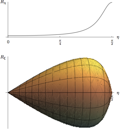
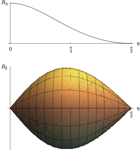
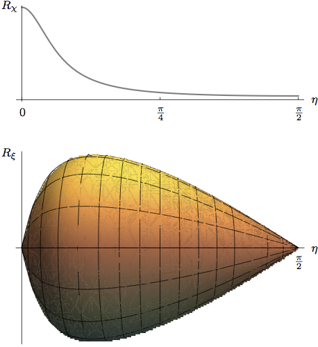
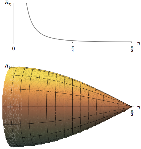
This describes a circle fibered non-trivially over a deformed sphere, which is illustrated schematically in figures 5(a), 5(b) and 5(c). The dual field strength is given by

\begin{split}\mathcal{H}=\beta\,\frac{\sin(2\eta)}{(\cos^{2}\eta+\beta^{2}\sin^{2}\eta)^{2}}\,d\chi\wedge d\xi\wedge d\eta\,.\end{split}

(5.19)

For $h=0$ , $\alpha=1$ and $\beta=0$ the resulting space becomes singular since the length of the Killing vector vanishes at $\eta=0$ , as illustrated in figure 5(d). Finally, for $h\neq 0$ and $\alpha^{2}\neq\beta^{2}$ the geometry is rather complicated and we do not present a detailed analysis here.

Before closing this section, let us also comment on the isometries for the T-dual background and remark that for $\alpha^{2}\neq\beta^{2}$ only two of the Killing vectors in (5.4) commute with (5.7), namely

\begin{split}k_{(1)}\hskip 40.0pt\mbox{and}\hskip 40.0ptk_{(2)}\,.\end{split}

(5.20)

This agrees with the fact that the metric (5.18) has only two directions of isometry, described by $k_{(\chi)}=\partial_{\chi}$ and $k_{(\xi)}=\partial_{\xi}$ .

5.2 Twisted sphere

Our aim in this section is to construct a non-geometric background via a T-duality transformation on the sphere. However, as we have seen in the last section, for the three-sphere the Killing vectors (5.4) are all globally defined. Similarly, after applying a T-duality transformation to $S^{3}$ , also the Killing vectors of the resulting background shown in (5.16) and below (5.20) do not exhibit monodromies of the form (4.27). Hence, we do not expect to find a non-geometric background by applying successive T-duality transformations to a single three-sphere.⁶⁶ 6 Following the reasoning of [62], this implies that, at least for a single three-sphere $S^{3}$ , no non-geometric fluxes should appear in the corresponding dimensionally-reduced theory.

But, let us recall from equation (5.2) that the three-sphere can be interpreted as a two-torus fibered over a line segment. If we then consider a four-dimensional space in which a circle is twisted over $S^{3}$ , we arrive at a situation similar to the twisted torus discussed in section 4.2.⁷⁷ 7 Note that, in contrast to the twisted torus, the second cohomology class of $S^{3}$ is trivial, and hence all circle bundles over $S^{3}$ are topological trivial. Nevertheless, a non-geometric background can be obtained. We thank the referee at JHEP for pointing this out to us. Therefore, in this case it appears to be possible to obtain a T-fold after an appropriate T-duality transformation.

Geometry

Let us specify the geometry of the four-dimensional space. Compared to section 5.1, we slightly change the parametrization of $S^{3}$ by substituting $\xi_{1,2}\to\xi_{1}\pm\xi_{2}$ in (5.2). The metric under consideration is then given by the following line-element squared

\begin{split}ds^{2}=R_{1}^{2}\,\Bigl[\,\bigl(\mathsf{E}^{\xi_{1}}\bigr)^{2}-2\cos(2\eta)\,\mathsf{E}^{\xi_{1}}\!\otimes\mathsf{E}^{\xi_{2}}+\bigl(\mathsf{E}^{\xi_{2}}\bigr)^{2}+(\mathsf{E}^{\eta})^{2}\,\Bigr]+R^{2}_{2}\bigl(\mathsf{E}^{X}\bigr)^{2}\,.\end{split}

(5.21)

The topology of the space is characterized by the one-forms $\{\mathsf{E}^{\xi_{1}},\mathsf{E}^{\xi_{2}},\mathsf{E}^{\eta},\mathsf{E}^{X}\}$ which satisfy the algebra

\begin{split}d\hskip 1.0pt\mathsf{E}^{\xi_{1}}=d\hskip 1.0pt\mathsf{E}^{\xi_{2}}=d\hskip 1.0pt\mathsf{E}^{\eta}=0\,,\hskip 60.0ptd\hskip 1.0pt\mathsf{E}^{X}=f\hskip 1.0pt\mathsf{E}^{\xi_{1}}\wedge\mathsf{E}^{\xi_{2}}\,.\end{split}

(5.22)

In local coordinates, these one-forms can be expressed as

\begin{split}\begin{array}[]{ll}\displaystyle\mathsf{E}^{\xi_{1}}&=d\xi_{1}\,,\\ \displaystyle\mathsf{E}^{\xi_{2}}&=d\xi_{2}\,,\\ \displaystyle\mathsf{E}^{\eta}&=d\eta\,,\\ \displaystyle\mathsf{E}^{X}&\displaystyle=dX+f\bigl(\rho_{1}\hskip 1.0pt\xi_{1}\hskip 1.0ptd\xi_{2}-\rho_{2}\hskip 1.0pt\xi_{2}\hskip 1.0ptd\xi_{1}\bigr)\,,\hskip 50.0pt\rho_{1}+\rho_{2}=1\,,\end{array}\end{split}

(5.23)

where the choice of local coordinates is parametrized by the constants $\rho_{1}$ and $\rho_{2}$ . Furthermore, we observe that if we require the one-forms (5.23) to be well-defined, we have to make the identifications

\begin{split}\begin{array}[]{c@{\hspace{15pt}}lcl@{\hspace{30pt}}lcl}1)\hfil\hskip 15.0&\xi_{1}&\rightarrow&\xi_{1}+2\pi\,,\hfil\hskip 30.&X&\rightarrow&X-2\pi\hskip 1.0ptf\rho_{1}\hskip 1.0pt\xi_{2}\,,\\ 2)\hfil\hskip 15.0&\xi_{2}&\rightarrow&\xi_{2}+2\pi\,,\hfil\hskip 30.&X&\rightarrow&X+2\pi\hskip 1.0ptf\rho_{2}\hskip 1.0pt\xi_{1}\,,\\ 3)\hfil\hskip 15.0&X&\rightarrow&X+2\pi\,.\hfil\hskip 30.\end{array}\end{split}

(5.24)

For our purposes in the following, three Killing vectors of the metric (5.21) are of interest. In terms of the vector fields $\{\mathsf{E}_{\xi_{1}},\mathsf{E}_{\xi_{2}},\mathsf{E}_{\eta},\mathsf{E}_{X}\}$ , dual to the corresponding one-forms, we have

\begin{split}\mathsf{K}_{(1)}=\mathsf{E}_{X}\,,\hskip 60.0pt\mathsf{K}_{(2)}&=\mathsf{E}_{\xi_{1}}-f\hskip 1.0pt\xi_{2}\hskip 1.0pt\mathsf{E}_{X}\,,\\[3.0pt] \mathsf{K}_{(3)}&=\mathsf{E}_{\xi_{2}}+f\hskip 1.0pt\xi_{1}\hskip 1.0pt\mathsf{E}_{X}\,.\end{split}

(5.25)

Note that these Killing vectors are not all globally defined. Indeed, under the identifications (5.24) we find the following monodromies

\begin{split}&\mathsf{K}_{(2)}\;\;\xrightarrow{\;\;\xi_{2}\to\xi_{2}+2\pi\;\;}\;\;\mathsf{K}_{(2)}-2\pi\hskip 1.0ptf\,\mathsf{K}_{(1)}\,,\\[3.0pt] &\mathsf{K}_{(3)}\;\;\xrightarrow{\;\;\xi_{1}\to\xi_{1}+2\pi\;\;}\;\;\mathsf{K}_{(3)}+2\pi\hskip 1.0ptf\,\mathsf{K}_{(1)}\,.\end{split}

(5.26)

T-duality along $\mathsf{K}_{(1)}$

Let us now consider a T-duality transformation along $\mathsf{K}_{(1)}$ on the above background. The metric is determined by (5.21), and we choose a vanishing field strength for the Kalb-Ramond field. In order to apply the T-duality rules from page 3.3, we first have to check whether the restrictions (3.30) are satisfied. This can be done by expressing $\mathsf{K}_{(1)}$ in a local basis as follows

\begin{split}\mathsf{K}_{(1)}=\partial_{X}\,,\end{split}

(5.27)

which indeed solves the above-mentioned constraints. When determining the dual metric, also the metric tensor has to be written in the basis $\{d\xi_{1},d\xi_{2},d\eta,dX\}$ , resulting in a rather lengthy expression which we do not display here. However, employing (3.26) together with (3.27), we find the following dual line-element squared

\begin{split}\mathsf{ds}^{2}=R_{1}^{2}\,\Bigl[\,(d\xi_{1})^{2}-2\cos(2\eta)\,d\xi_{1}\otimes d\xi_{2}+(d\xi_{2})^{2}+(d\eta)^{2}\,\Bigr]+\frac{1}{R_{2}^{2}}\,(d\chi)^{2}\,.\end{split}

(5.28)

The T-dual field strength can be determined from equation (3.28) and reads

\begin{split}\mathcal{H}=f\hskip 1.0ptd\xi_{1}\wedge d\xi_{2}\wedge d\chi\,.\end{split}

(5.29)

Therefore, the background obtained after applying a T-duality transformation on the twisted sphere along $\mathsf{K}_{(1)}$ is given by $S^{3}\times S^{1}$ , with a non-vanishing field strength $\mathcal{H}$ .

T-duality along $\mathsf{K}_{(2)}$

We now turn to the Killing vector $\mathsf{K}_{(2)}$ . Even though $\mathsf{K}_{(2)}$ is not single valued, we proceed along similar lines as in section 4.2 and perform a T-duality transformation on the geometry (5.21) locally. This then leads to a non-geometric space, which is only locally geometric. Note that the field strength $H$ of the Kalb-Ramond field is again chosen to be vanishing.

As in the previous examples, in order to apply the transformation rules, we have to express the metric and Killing vectors in local coordinates. For the latter, we find

\begin{split}\mathsf{K}_{(2)}=\partial_{\xi_{1}}-f\rho_{1}\hskip 1.0pt\xi_{2}\hskip 1.0pt\partial_{X}\,,\end{split}

(5.30)

and thus the constraints in (3.30) are only satisfied for geometries specified by $\rho_{1}=0$ and $\rho_{2}=1$ . In this case, the metric in local coordinates $\{d\xi_{1},d\xi_{2},d\eta,dX\}$ simplifies and takes the following form

\begin{split}\widetilde{G}_{ij}=\left(\begin{array}[]{cccc}R_{1}^{2}+R_{2}^{2}\hskip 1.0ptf^{2}\xi_{2}^{2}&-R_{1}^{2}\cos(2\eta)&0&-R_{2}^{2}f\xi_{2}\\ -R_{1}^{2}\cos(2\eta)&R_{1}^{2}&0&0\\ 0&0&R_{1}^{2}&0\\ -R_{2}^{2}f\xi_{2}&0&0&R_{2}^{2}\end{array}\right),\end{split}

(5.31)

where $i,j\in\{\xi_{1},\xi_{2},\eta,X\}$ . Applying then the transformation rules given in equation (3.26), we find the following dual line-element squared

\begin{split}\mathsf{ds}^{2}=R_{1}^{2}\Bigl[\hskip 1.0pt(d\eta)^{2}+\sin^{2}(2\eta)(d\xi)^{2}\hskip 1.0pt\Bigr]+\vartheta(\xi)\left[\,\tfrac{1}{R_{1}^{2}}\,(d\chi)^{2}+R_{2}^{2}\hskip 1.0pt\Bigl(dX-\cos(2\eta)f\hskip 1.0pt\xi\hskip 1.0ptd\xi\Bigr)^{2}\right],\end{split}

(5.32)

where we simplified our notation by replacing $\xi_{2}\to\xi$ , and where we have defined the function

\begin{split}\vartheta(\xi)=\frac{1}{1+\bigl(\frac{R_{2}}{R_{1}}f\xi\bigr)^{2}}\,.\end{split}

(5.33)

The non-vanishing components of the dual field strength, determined via the equations in (3.28), read

\begin{split}\mathcal{H}_{\eta\xi\chi}=2\sin(2\eta)\hskip 1.0pt\vartheta(\xi)\,,\hskip 45.0pt\mathcal{H}_{X\xi\chi}=-f\left(\frac{R_{2}}{R_{1}}\right)^{2}\vartheta^{2}(\xi)\hskip 1.0pt\Bigl[1-\bigl(\tfrac{R_{2}}{R_{1}}\hskip 1.0ptf\hskip 1.0pt\xi\bigr)^{2}\Bigr]\,.\end{split}

(5.34)

Note that this background is locally geometric, but is globally not well-defined. Indeed, when going around the circle in the $\xi$ -direction as $\xi\to\xi+2\pi$ , the metric given by (5.32) and the components of the field strength (5.34) are not periodic. The mismatch cannot be compensated by having diffeomorphism as transition functions between different charts, since the former is due to the monodromy (5.26) of the Killing vector $\mathsf{K}_{(2)}$ . However, following the same reasoning as illustrated in figure 4, the dual space can be interpreted as a T-fold.

5.3 T-fold

It is beyond the scope of this paper to analyze the above T-fold background in further detail, and we refer this question to a later point. Nevertheless, let us make the following remarks. In order to simplify the metric in (5.32), we introduce as basis of one-forms as follows

\begin{split}&\mathbb{E}^{\xi}=d\xi\,,\\ &\mathbb{E}^{\eta}=d\eta\,,\hskip 60.0pt\mathbb{E}^{X}=dX-f\cos(2\eta)\hskip 1.0pt\xi\hskip 1.0ptd\xi\,,\\[2.0pt] &\mathbb{E}^{\chi}=d\chi\,,\end{split}

(5.35)

where in particular $\mathbb{E}^{X}$ is not single-valued and not closed

\begin{split}d\mathbb{E}^{\xi}=d\mathbb{E}^{\eta}=d\mathbb{E}^{\chi}=0\,,\hskip 60.0ptd\mathbb{E}^{X}=2f\sin(2\eta)\hskip 1.0pt\xi\hskip 1.0ptd\eta\wedge d\xi\,.\end{split}

(5.36)

Employing this basis, the metric of the T-fold can be expressed via the following line-element squared as

\begin{split}ds^{2}=R_{1}^{2}\Bigl[\hskip 1.0pt\bigl(\mathbb{E}^{\eta}\bigr)^{2}+\sin^{2}(2\eta)\bigl(\mathbb{E}^{\xi}\bigr)^{2}\hskip 1.0pt\Bigr]+\vartheta(\xi)\left[\,\tfrac{1}{R_{1}^{2}}\,\bigl(\mathbb{E}^{\chi}\bigr)^{2}+R_{2}^{2}\hskip 1.0pt\bigl(\mathbb{E}^{X}\bigr)^{2}\right],\end{split}

(5.37)

where the function $\vartheta(\xi)$ was defined in equation (5.33). The line element (5.37) describes a local two-torus $\widetilde{\mathbb{T}}^{2}$ along $\mathbb{E}^{\chi}$ and $\mathbb{E}^{X}$ , which is non-trivially fibered over a two-sphere. We also remark that for a vanishing twisting $f=0$ , we obtain the geometric background $S^{2}\times\mathbb{T}^{2}$ .

Chain of T-duality transformations

Let us finally summarize the chain of T-duality transformations studied in this section. After slightly adjusting our notation and denoting by $\mathcal{E}_{h}$ and $\widetilde{\mathcal{E}}_{h}$ the global and local circle bundles with twisting $h$ discussed above, we arrive at the following picture:

\begin{split}\begin{array}[]{c@{\hspace{10pt}}||r@{\hspace{4pt}}c@{\hspace{-22pt}}c@{\hspace{-22pt}}c@{\hspace{5pt}}l@{\hspace{35pt}}l}\mbox{background}\hfil\hskip 10.&\lx@intercol\hfil\mbox{geometry}\hfil\lx@intercol&\mbox{field strength}\\ \hline\cr\hline\cr\hfil\hskip 10.&\hskip 4.0&\hfil\hskip-22.0\\[-5.0pt] \mbox{$H$-flux}\hfil\hskip 10.&\hskip 4.0&\hfil\hskip-22.0&\hskip 7.0ptS^{1}_{X}\>\times\>S^{3}_{\xi_{1},\xi_{2},\eta}\hfil\hskip-22.0&\hfil\hskip 5.0&\hfil\hskip 35.0&H=h\,d\xi_{1}\wedge d\xi_{2}\wedge dX\\ \hfil\hskip 10.&\hskip 4.0&\hfil\hskip-22.0&\hskip 6.0pt\rotatebox{270.0}{$\displaystyle\xleftrightarrow{\hskip 8.19447pt\rotatebox{90.0}{$\scriptstyle\mathsf{T}_{X}$}\hskip 8.19447pt}$}\hfil\hskip-22.0\\[43.0pt] \mbox{$f$-flux}\hfil\hskip 10.&S^{1}_{X}\hskip 4.0&\hookrightarrow\hfil\hskip-22.0&\mathcal{E}_{h}\hfil\hskip-22.0&\rightarrow\hfil\hskip 5.0&S^{3}_{\xi_{1},\xi_{2},\eta}\hfil\hskip 35.0&H=0\\ \hfil\hskip 10.&\hskip 4.0&\hfil\hskip-22.0&\hskip 6.5pt\rotatebox{270.0}{$\displaystyle\xleftrightarrow{\hskip 8.19447pt\rotatebox{90.0}{$\scriptstyle\mathsf{T}_{\xi_{1}}$}\hskip 8.19447pt}$}\hfil\hskip-22.0\\[43.0pt] \mbox{$Q$-flux}\hfil\hskip 10.&\hskip 10.0pt\widetilde{\mathbb{T}}_{X,\xi_{1}}\hskip 4.0&\hookrightarrow\hfil\hskip-22.0&\widetilde{\mathcal{E}}_{h}\hfil\hskip-22.0&\rightarrow\hfil\hskip 5.0&S^{2}_{\xi_{2},\eta}\hfil\hskip 35.0&\widetilde{H}\neq 0\\ \hfil\hskip 10.&\hskip 4.0&\hfil\hskip-22.0&\hskip 6.5pt\rotatebox{270.0}{$\displaystyle\xleftrightarrow{\hskip 8.19447pt\rotatebox{90.0}{$\scriptstyle\mathsf{T}_{\xi_{2}}$}\hskip 8.19447pt}$}\hfil\hskip-22.0\\[43.0pt] \mbox{$R$-flux}\hfil\hskip 10.&\hskip 4.0&\hfil\hskip-22.0&\hskip-5.0pt\ldots\hfil\hskip-22.0\\[-8.0pt] \hfil\hskip 10.&\hskip 4.0&\hfil\hskip-22.0&\hfil\hskip-22.0&\hfil\hskip 5.0&\hfil\hskip 35.0&{\color[rgb]{1,1,1}\cdot}\end{array}\end{split}

(5.38)

Given these relations, it is then tempting to speculate that a further T-duality transformation on the T-fold gives rise to an $R$ -flux background with non-associative features. However, as we mentioned above, this discussion is beyond the scope of this paper.

6 Summary and conclusions

In this paper, we have reviewed the transformation rules of the metric, Kalb-Ramond field and dilaton under T-duality. However, instead of expressing the formulas in terms of the Kalb-Ramond field $B$ itself, as it is usually done for the Buscher rules, we described the T-dual background employing the corresponding field strength $H=dB$ . In sections 4 and 5 we have then illustrated our formalism with a detailed discussion of T-duality transformations for tori and spheres.

The Buscher rules have long been studied in the literature from different perspectives, and are rather well-understood. Nevertheless, in this paper we were able derive some novel results and provide new interpretations on this subject.

•

In particular, in section 2 we reviewed the sigma-model action for the closed string for a non-vanishing field strength $H$ of the Kalb-Ramond field. We found that the symmetry structure of this action can be described via the $H$ -twisted Courant bracket, which agrees with similar results in [54] obtained in a different context.
•

In section 3 we derived the transformation rules of the metric, Kalb-Ramond field and dilaton under T-duality. This was done through gauging the sigma-model action by a target-space isometry. We then observed that the remaining global symmetries of the gauged action are determined by (3.9). This explains how under T-duality the isometry group can be reduced, which we illustrated with examples in sections 4.3 and 5.1.
•

In the course of the derivation of the T-duality rules, we made us of an enlarged target space [61, 62], for which a metric $\check{G}$ and field strength $\check{H}$ can be defined. We noted that the metric $\check{G}$ has a null-eigenvector, which can be used to obtain a convenient set of coordinates leading to a dual target-space background. However, this can only be done consistently if the constraint (3.25) is met. For many examples (3.25) is automatically satisfied, but we believe that this restriction has not appeared in the literature until now.
•

In contrast to the Buscher rules given for the metric $G$ and Kalb-Ramond field $B$ , here we expressed the T-duality transformation rules in terms of $G$ and the field strength $H=dB$ . ⁸⁸ 8 T-duality transformation rules involving the field strength $H$ have also appeared in [67], but without a detailed derivation from a world-sheet point of view. This has the advantage that we do not have to rely on a choice of gauge for the initial configuration. For the dual background, the topology is specified by the $H$ -flux, and for the geometry there is a freedom of choosing local coordinates. This is in accordance with the Buscher rules, where a choice of gauge for $B$ determines the dual geometry.
•

In section 4 we have illustrated the above-mentioned transformation rules with the example of the three-torus. The results obtained in our formalism agree with those known in the literature, however, we were able to generalize these findings by allowing for instance for general T-duality directions. We furthermore discussed possible monodromies of Killing vectors, and in figure 4 we interpreted the T-fold from a point of view which does not involve a doubled geometry.
•

Finally, in section 5 we studied T-duality transformations for spheres. We first reviewed and generalized the discussion in [62] about the three-sphere, and then constructed a new example of a non-geometric background.

The results obtained in this paper motivate further studies in this direction. First, it would be interesting to study the T-fold based on the sphere as a supergravity background, and investigate whether conclusions similar to those in [9] can be drawn. Furthermore, the approach to analyze T-duality transformations presented here might be suitable to find new non-geometric backgrounds which are not based on the torus. Second, since the sigma model on a three-sphere with $H$ -flux corresponds to the $SU(2)$ WZW model, which is conformal, it might be possible to investigate the T-fold of section 5 as a proper string-theory background. This could lead to a better string-theoretical understanding of non-geometric spaces. We hope to return to these questions in the future.

Acknowledgements

We would like to thank Ralph Blumenhagen, Gianguido Dall’Agata, Luca Martucci and especially Felix Rennecke for very helpful discussions, furthermore Gianguido Dall’Agata for useful comments on the manuscript, and Larisa Jonke for correspondence on the Jacobiator of the $H$ -twisted Courant bracket. We also thank the referee at JHEP for helpful comments. The author is supported by the MIUR grants PRIN 2009-KHZKRX and FIRB RBFR10QS5J.

References

[1] A. Giveon, M. Porrati, and E. Rabinovici, “Target space duality in string theory,” Phys.Rept. 244 (1994) 77–202, hep-th/9401139.
[2] J. Scherk and J. H. Schwarz, “Spontaneous Breaking of Supersymmetry Through Dimensional Reduction,” Phys.Lett. B82 (1979) 60.
[3] J. Scherk and J. H. Schwarz, “How to Get Masses from Extra Dimensions,” Nucl.Phys. B153 (1979) 61–88.
[4] K. Dasgupta, G. Rajesh, and S. Sethi, “M theory, orientifolds and G - flux,” JHEP 9908 (1999) 023, hep-th/9908088.
[5] S. Kachru, M. B. Schulz, P. K. Tripathy, and S. P. Trivedi, “New supersymmetric string compactifications,” JHEP 0303 (2003) 061, hep-th/0211182.
[6] S. Hellerman, J. McGreevy, and B. Williams, “Geometric constructions of nongeometric string theories,” JHEP 0401 (2004) 024, hep-th/0208174.
[7] A. Dabholkar and C. Hull, “Duality twists, orbifolds, and fluxes,” JHEP 0309 (2003) 054, hep-th/0210209.
[8] C. Hull, “A Geometry for non-geometric string backgrounds,” JHEP 0510 (2005) 065, hep-th/0406102.
[9] J. Shelton, W. Taylor, and B. Wecht, “Nongeometric flux compactifications,” JHEP 0510 (2005) 085, hep-th/0508133.
[10] V. Mathai and J. M. Rosenberg, “T duality for torus bundles with H fluxes via noncommutative topology,” Commun.Math.Phys. 253 (2004) 705–721, hep-th/0401168.
[11] V. Mathai and J. M. Rosenberg, “On Mysteriously missing T-duals, H-flux and the T-duality group,” hep-th/0409073.
[12] P. Grange and S. Schäfer-Nameki, “T-duality with H-flux: Non-commutativity, T-folds and G x G structure,” Nucl.Phys. B770 (2007) 123–144, hep-th/0609084.
[13] D. Lüst, “T-duality and closed string non-commutative (doubled) geometry,” JHEP 1012 (2010) 084, 1010.1361.
[14] D. Lüst, “Twisted Poisson Structures and Non-commutative/non-associative Closed String Geometry,” PoS CORFU2011 (2011) 086, 1205.0100.
[15] C. Condeescu, I. Florakis, and D. Lüst, “Asymmetric Orbifolds, Non-Geometric Fluxes and Non-Commutativity in Closed String Theory,” JHEP 1204 (2012) 121, 1202.6366.
[16] A. Chatzistavrakidis and L. Jonke, “Matrix theory origins of non-geometric fluxes,” JHEP 1302 (2013) 040, 1207.6412.
[17] D. Andriot, M. Larfors, D. Lüst, and P. Patalong, “(Non-)commutative closed string on T-dual toroidal backgrounds,” JHEP 1306 (2013) 021, 1211.6437.
[18] I. Bakas and D. Lüst, “3-Cocycles, Non-Associative Star-Products and the Magnetic Paradigm of R-Flux String Vacua,” 1309.3172.
[19] P. Bouwknegt, K. Hannabuss, and V. Mathai, “Nonassociative tori and applications to T-duality,” Commun.Math.Phys. 264 (2006) 41–69, hep-th/0412092.
[20] P. Bouwknegt, K. Hannabuss, and V. Mathai, “T-duality for principal torus bundles and dimensionally reduced Gysin sequences,” Adv.Theor.Math.Phys. 9 (2005) 749–773, hep-th/0412268.
[21] I. Ellwood and A. Hashimoto, “Effective descriptions of branes on non-geometric tori,” JHEP 0612 (2006) 025, hep-th/0607135.
[22] R. Blumenhagen and E. Plauschinn, “Nonassociative Gravity in String Theory?,” J.Phys.A A44 (2011) 015401, 1010.1263.
[23] R. Blumenhagen, A. Deser, D. Lüst, E. Plauschinn, and F. Rennecke, “Non-geometric Fluxes, Asymmetric Strings and Nonassociative Geometry,” J.Phys. A44 (2011) 385401, 1106.0316.
[24] R. Blumenhagen, “Nonassociativity in String Theory,” 1112.4611.
[25] D. Mylonas, P. Schupp, and R. J. Szabo, “Membrane Sigma-Models and Quantization of Non-Geometric Flux Backgrounds,” JHEP 1209 (2012) 012, 1207.0926.
[26] E. Plauschinn, “Non-geometric fluxes and non-associative geometry,” PoS CORFU2011 (2011) 061, 1203.6203.
[27] A. Flournoy, B. Wecht, and B. Williams, “Constructing nongeometric vacua in string theory,” Nucl.Phys. B706 (2005) 127–149, hep-th/0404217.
[28] A. Flournoy and B. Williams, “Nongeometry, duality twists, and the worldsheet,” JHEP 0601 (2006) 166, hep-th/0511126.
[29] S. Hellerman and J. Walcher, “Worldsheet CFTs for Flat Monodrofolds,” hep-th/0604191.
[30] C. Condeescu, I. Florakis, C. Kounnas, and D. Lüst, “Gauged supergravities and non-geometric Q/R-fluxes from asymmetric orbifold CFT’s,” 1307.0999.
[31] A. Dabholkar and C. Hull, “Generalised T-duality and non-geometric backgrounds,” JHEP 0605 (2006) 009, hep-th/0512005.
[32] C. M. Hull, “Doubled Geometry and T-Folds,” JHEP 0707 (2007) 080, hep-th/0605149.
[33] D. Andriot, M. Larfors, D. Lüst, and P. Patalong, “A ten-dimensional action for non-geometric fluxes,” JHEP 1109 (2011) 134, 1106.4015.
[34] D. Andriot, O. Hohm, M. Larfors, D. Lüst, and P. Patalong, “A geometric action for non-geometric fluxes,” Phys.Rev.Lett. 108 (2012) 261602, 1202.3060.
[35] D. Andriot, O. Hohm, M. Larfors, D. Lüst, and P. Patalong, “Non-Geometric Fluxes in Supergravity and Double Field Theory,” Fortsch.Phys. 60 (2012) 1150–1186, 1204.1979.
[36] R. Blumenhagen, A. Deser, E. Plauschinn, and F. Rennecke, “A bi-invariant Einstein-Hilbert action for the non-geometric string,” Phys.Lett. B720 (2013) 215–218, 1210.1591.
[37] R. Blumenhagen, A. Deser, E. Plauschinn, and F. Rennecke, “Non-geometric strings, symplectic gravity and differential geometry of Lie algebroids,” JHEP 1302 (2013) 122, 1211.0030.
[38] R. Blumenhagen, A. Deser, E. Plauschinn, F. Rennecke, and C. Schmid, “The Intriguing Structure of Non-geometric Frames in String Theory,” 1304.2784.
[39] D. Andriot and A. Betz, “ $\beta$ -supergravity: a ten-dimensional theory with non-geometric fluxes, and its geometric framework,” 1306.4381.
[40] N. Halmagyi, “Non-geometric String Backgrounds and Worldsheet Algebras,” JHEP 0807 (2008) 137, 0805.4571.
[41] N. Halmagyi, “Non-geometric Backgrounds and the First Order String Sigma Model,” 0906.2891.
[42] G. Aldazabal, D. Marques, and C. Nunez, “Double Field Theory: A Pedagogical Review,” Class.Quant.Grav. 30 (2013) 163001, 1305.1907.
[43] O. Hohm, D. Lüst, and B. Zwiebach, “The Spacetime of Double Field Theory: Review, Remarks, and Outlook,” 1309.2977.
[44] E. Witten, “Nonabelian Bosonization in Two-Dimensions,” Commun.Math.Phys. 92 (1984) 455–472.
[45] D. Gepner and E. Witten, “String Theory on Group Manifolds,” Nucl.Phys. B278 (1986) 493.
[46] P. Bouwknegt, J. Evslin, and V. Mathai, “T duality: Topology change from H flux,” Commun.Math.Phys. 249 (2004) 383–415, hep-th/0306062.
[47] T. Buscher, “Quantum Corrections and Extended Supersymmetry in New $\sigma$ Models,” Phys.Lett. B159 (1985) 127.
[48] T. Buscher, “A Symmetry of the String Background Field Equations,” Phys.Lett. B194 (1987) 59.
[49] T. Buscher, “Path Integral Derivation of Quantum Duality in Nonlinear Sigma Models,” Phys.Lett. B201 (1988) 466.
[50] E. Witten, “Global Aspects of Current Algebra,” Nucl.Phys. B223 (1983) 422–432.
[51] C. Hull and B. J. Spence, “The Gauged Nonlinear Sigma Model With Wess-Zumino Term,” Phys.Lett. B232 (1989) 204.
[52] C. Hull and B. J. Spence, “The Geometry of the gauged sigma model with Wess-Zumino term,” Nucl.Phys. B353 (1991) 379–426.
[53] D. M. Belov, C. M. Hull, and R. Minasian, “T-duality, gerbes and loop spaces,” 0710.5151.
[54] A. Alekseev and T. Strobl, “Current algebras and differential geometry,” JHEP 0503 (2005) 035, hep-th/0410183.
[55] N. Hitchin, “Generalized Calabi-Yau manifolds,” Quart.J.Math.Oxford Ser. 54 (2003) 281–308, math/0209099.
[56] M. Gualtieri, “Generalized complex geometry,” math/0401221.
[57] M. Grana, R. Minasian, M. Petrini, and D. Waldram, “T-duality, Generalized Geometry and Non-Geometric Backgrounds,” JHEP 0904 (2009) 075, 0807.4527.
[58] C. Hull and B. Zwiebach, “The Gauge algebra of double field theory and Courant brackets,” JHEP 0909 (2009) 090, 0908.1792.
[59] P. Severa and A. Weinstein, “Poisson geometry with a 3 form background,” Prog.Theor.Phys.Suppl. 144 (2001) 145–154, math/0107133.
[60] I. Jack, D. Jones, N. Mohammedi, and H. Osborn, “Gauging the General $\sigma$ Model With a Wess-Zumino Term,” Nucl.Phys. B332 (1990) 359.
[61] M. Rocek and E. P. Verlinde, “Duality, quotients, and currents,” Nucl.Phys. B373 (1992) 630–646, hep-th/9110053.
[62] E. Alvarez, L. Alvarez-Gaume, J. Barbon, and Y. Lozano, “Some global aspects of duality in string theory,” Nucl.Phys. B415 (1994) 71–100, hep-th/9309039.
[63] J. M. Figueroa-O’Farrill and S. Stanciu, “Equivariant cohomology and gauged bosonic sigma models,” hep-th/9407149.
[64] C. Hull, “Global aspects of T-duality, gauged sigma models and T-folds,” JHEP 0710 (2007) 057, hep-th/0604178.
[65] P. Bouwknegt, J. Evslin, and V. Mathai, “On the topology and H flux of T dual manifolds,” Phys.Rev.Lett. 92 (2004) 181601, hep-th/0312052.
[66] P. Bouwknegt, K. Hannabuss, and V. Mathai, “T duality for principal torus bundles,” JHEP 0403 (2004) 018, hep-th/0312284.
[67] I. A. Bandos and B. Julia, “Superfield T duality rules,” JHEP 0308 (2003) 032, hep-th/0303075.

Abstract

1 Introduction

2 Sigma-model action for the closed string

Action

Invariance under field redefinitions

Algebraic structure of field redefinitions

3 T-duality

3.1 Gauging a symmetry

The gauged action

Remarks

Multiple global symmetries

3.2 Integrating out the gauge field

World-sheet action for the enlarged target-space

Killing vector

Adapted coordinates

3.3 Transformation rules

Final results

Remarks

4 Examples I – Tori

4.1 Torus

Symmetry structure

T-duality transformation

Choice of a local geometry

Remarks

4.2 Twisted torus

Killing vectors

T-duality along k(1)k_{(1)}

T-duality along k(2)k_{(2)}

Transition functions

4.3 T-fold

Remark

5 Examples II – Spheres

5.1 Sphere

Killing vectors

T-duality

Backgrounds with α2=β2\alpha^{2}=\beta^{2}

Backgrounds with α2≠β2\alpha^{2}\neq\beta^{2}

5.2 Twisted sphere

Geometry

T-duality along 𝖪(1)\mathsf{K}_{(1)}

T-duality along 𝖪(2)\mathsf{K}_{(2)}

5.3 T-fold

Chain of T-duality transformations

6 Summary and conclusions

Acknowledgements

References

T-duality along $k_{(1)}$

T-duality along $k_{(2)}$

Backgrounds with $\alpha^{2}=\beta^{2}$

Backgrounds with $\alpha^{2}\neq\beta^{2}$

T-duality along $\mathsf{K}_{(1)}$

T-duality along $\mathsf{K}_{(2)}$