Homogenization of the spectral equation in one-dimension
Abstract
The asymptotic behavior of a one-dimensional spectral problem with periodic coefficient is addressed for high frequency modes by a method of Bloch wave homogenization. The analysis leads to a spectral problem including both microscopic and macroscopic eigenmodes. Numerical simulation results are provided to corroborate the theory.
Keywords. Homogenization, Bloch waves, spectral problem, two-scale transform.
1 Introduction
We consider the spectral problem
| (1) |
posed in an one-dimensional open bounded domain with Dirichlet boundary conditions. An asymptotic analysis of this problem is carried out where is a parameter tending to zero and the coefficients are -periodic, namely and where and are -periodic in . The homogenization of such spectral problem has been studied in various works providing the asymptotic behaviour of eigenvalues and eigenvectors. The low frequency part of the spectrum has been investigated in [17], [18], [25]. Then, many configurations have been analyzed, as [16] and [13] for a fluid-structure interaction, [7], [3] for neutron transport, [22], [24] for which changes sign or [4] for the first high frequency eigenvalue and eigenvector for a one-dimensional non-self-adjoint problem with Neumann boundary conditions. In [6], G. Allaire and C. Conca studied the asymptotic behaviour of both the low and high frequency spectrum. In order to analyze the asymptotic behaviour of the high frequency eigenvalues, they used the Bloch wave homogenization method. It is a blend of two-scale convergence, see e.g. [1], [2], [21], and Bloch wave decomposition, see e.g. [15], [12], [14], and was previously introduced in [5] to a fluid-solid interaction problem. They have shown that the limit of the set of renormalized eigenvalues is the union of the Bloch spectrum and the boundary layer spectrum, when goes to . However, the asymptotic behaviour of the corresponding eigenvectors was not addressed. This is the goal of the present work which focuses on the Bloch spectrum of the high frequency part. Precisely, we search eigenvalues such that
| (2) |
where is solution of the Bloch wave spectral problem, also called the microscopic equation in this work,
| (3) |
with quasi-periodic boundary conditions for some . From [6], it is known that each can be reached as a limit of a subsequence of . For each and each is either a simple or a double eigenvalue and . We pose if and otherwise. To guarantee that Bloch waves are kept in the weak limit, we apply the modulated two-scale transform , defined in [8] from the usual two-scale transform in [20], [19], [10], [9] or [11]. Passing to the limit in the weak formulation, it is shown that is weakly converging to two-scale modes
where the second sum runs over all modes with the same eigenvalue . Here, the modes are called microscopic modes. The factors are solution of the macroscopic system of first order differential equation,
| (4) |
which boundary conditions and the constant are depending on the involved microscopic modes and eigenvalues. The physical solution is then approximated by two-scale modes
| (5) |
These results are established for Neumann boundary conditions.
In fact, this method is inspired from [8] dedicated to the wave equation, except that in the latter work the two-scale transforms and were analyzed separately and the macroscopic boundary conditions were lacking. Moreover, the model derivation in [8] is starting from the wave equation written as a first order system. So, for the sake of comparison, we derive the homogenized spectral equation from a first order formulation.
In addition, we report exploration results regarding approximations of physical eigenmodes by two-scale modes. First, for a given and each high frequency physical eigenelement , we show how to find quadruplets satisfying the approximations (2) and (5). This shows that each high frequency eigenelement can be approximated by a two-scale mode. Conversely, the high-frequency physical eigenelements can be built from the two-scale eigenelements only. Namely, for a given Bloch mode , a macroscopic eigenelement is minimizing the error on the physical equation (1) where and are replaced by their approximations (2) and (5).
This paper is organized as follows. In Section 2 we state the physical spectral equation with Dirichlet boundary conditions. In Section 3 the notations and elementary properties, which are used throughout the paper, are introduced. In Section 4 and 5, the model homogenization is derived based on the second order and first order formulations respectively. Finally, the numerical results are reported in the last section.
2 Statement of the problem
We consider an interval, which boundary is denoted by , and two functions assumed to obey a prescribed profile,
| (6) |
where , are both -periodic where is an open interval. Moreover, they are required to satisfy the standard uniform positivity and ellipticity conditions:
| (7) |
for some given strictly positive , , and .
With the operators , the spectral problem with Dirichlet boundary conditions is
| (8) |
where as usual denotes a small parameter intended to go to zero.
The eigenvectors are normalized by
| (9) |
and we search the eigenvalues such that
| (10) |
where is a non negative real number and tends to zero with . The weak formulation of the spectral problem (8) is: find such that
| (11) |
Since is bounded, it results the uniform bound
| (12) |
3 Notations and elementary properties
The functional space of square integrable functions is over . Let and be -dimensional complex vector valued functions in , the dot product is denoted by and the hermitian inner product by
| (13) |
The notation refers to numbers or functions tending to zeros when in a sense made precise in each case. The notations are for and derivatives of a function . The vectors , are the outer unit normals of and
Bloch decomposition We follow the definition of Bloch decomposition in [8] with , , and , so The dual lattice is necessarily , and the equivalence class is chosen as . For , considering the dual lattices and we pose
so that . Posing yields .
Functional spaces of quasi-periodic functions For any , we define the quasi-periodic vector space over with the hermitian inner product (13) by
or equivalently
where is the traditional notation for in the periodic case i.e. when Likewise, for we set
bearing in mind that the subscript would be more appropriate in the periodic case
The modulated two-scale transform Let us assume from now that the domain is the union of a finite number of entire cells of size or equivalently that the sequence is exactly for . Setting is the set of all cells of .
Definition 1
For any , the modulated two-scale transform of the function , is defined by
| (14) |
where stands for the unique node in of and is the characteristic function of .
The three following properties can be checked by using (14) and are admitted. For
| (15) | |||
Remark 2
Let and a sequence bounded in such that converges to in weakly when , then converges to some in weakly. Moreover, since and are conjugate then and are also conjugate.
The adjoint of , is defined by
| (16) |
for all and , and we denote by the operator operating on functions defined in ,
| (17) |
The next Lemma shows that is an approximation of for quasi-periodic functions.
Lemma 3
Let a quasi-periodic function in then
| (18) |
Proof. The proof is carried out in two steps. First the explicit expression of is derived, then the approximation is deduced.
(i) Let us prove that
From the definition of the two-scale transform with ,
or equivalently,
Changing the variable names and using the definition of ,
This establishes the explicit expression of .
(ii) Let us derive the expected approximation for and quasi-periodic in . Since and
then
for a.e. and all . Remarking that and
So for all and ,
Therefore,
Using the quasi-periodic of in ,
in , hence the formula (18) follows.
In the proof, we constantly use the following consequence.
Corollary 4
Let and quasi-periodic in , for any sequence bounded in such that converges to in weakly when then
Two-scale operators For a function defined in we pose
so that
| (19) |
Bloch waves For a given , we denote by the Bloch wave eigenelements indexed by that are solution to
| (20) |
The corresponding weak formulation is: find solution to
| (21) |
Since the operator is self-adjoint, its spectra is real. Furthermore, for , we introduce the coefficients
| (22) |
and observe that the following properties hold,
and
In particular for , if the eigenvectors are chosen as real functions thus In the special case , for and otherwise.
Notation 5
For , , the conjugate of , is solution of . We choose the numbering of eigenvectors so that and remark that
Remark 6
In one dimension, for it is well-known that all eigenvalue are simple, except for where they are double.
Finally, we denote
4 Homogenization of the high-frequency eigenvalue problem
For , we decompose
| (23) |
and assume that the sequence of the is varying in a set depending on so that
| (24) |
We note that for , , so and .
4.1 Main result
The macroscopic equation is stated for each and each Bloch wave eigenvalue . For , we assume that for each , so it is stated as an eigenvalue problem
| (25) |
for each , with the boundary conditions
| (26) |
where is defined in (24). We observe that the first order operator of this system is self-adjoint on the domain
so is real.
For , assuming that is a double eigenvalue corresponding to two eigenvectors and , and that , the macroscopic system states
| (27) |
with the boundary conditions
| (28) |
Again since is self-adjoint on
Remark 7
(i) If for or for all varying in the macroscopic equations (25) or (27) are or . But is impossible since for all eigenmodes . So and this model does not provide any equation for .
(ii) For , if then and is a periodic solution that is a solution of . So, we consider always that for .
(iii) For , in case where the boundary conditions of the macroscopic equation vanishes.
Remark 8
This work focuses on the Bloch spectrum. To avoid eigenmodes related to the boundary spectrum, according to Proposition 7.7 in [6] we shall assume that the weak limit of in is not vanishing.
The main Theorem states as follows.
Theorem 9
For let be solution of (8) then is bounded in . For , as in (23, 24), assuming that the weak limit of in is non-vanishing and the renormalized sequence satisfies the decomposition (10), there exists such that with an eigenvalue of the Bloch wave spectrum and the limit of any weakly converging extracted subsequence of in can be decomposed on the Bloch modes
| (29) |
Moreover, and are solutions of the macroscopic equations (25, 26) and (27, 28). Finally, and are conjugate.
Thus, it follows from (29) that the physical solution is approximated by two-scale modes
| (30) |
The boundary conditions (26) and (28) can be directly derived by replacing in the physical boundary condition by its approximations,
| (31) |
For , they result from
and the assumption . For , the conditions follow from the periodicity of . Furthermore, we observe that and are generally not vanishing except for .
Proposition 10
Proof. For , , if the macroscopic solution is constant then and are constant for all and such that . Now, we consider and the proof is similar for . Based on Remark 14 about the macroscopic solutions in Section 4.4, is equivalent to . From the quasi-periodicity of ,
then is periodic or anti-periodic for . Hence is a solution of the equation
| (32) | |||
and is also a solution of (32). Denote by and observe that is a solution of the equation
with the boundary conditions
Finally, Proposition 10 is concluded.
Remark 11
The converse is probably true, and is numerically studied in Section 6.2, i.e. for any solution to (8), there exist , and two complex numbers and such that and
| (33) |
for two numbers such that the boundary conditions (28), respectively (26), are satisfied for respectively for . In the later case and are conjugate.
Remark 12
(i) The case of non-constant coefficients is used for approximations of the solution to the homogenized wave equation that may be derived from [8]. In such case belongs to a finite subset of made with values distant from and including . We cannot expect that there always exists a pair such that is a constant.
(ii) The case of non-constant coefficients is also seen as a preparation to derive homogenized spectral problems in higher dimension where the boundary conditions constitute a more difficult problem and may require a more general solution than constant .
Proof of Theorem 9
Proof. The proof is based on Lemma 13 in Section 4.2 and on the macroscopic model derivation in Section 4.3. For a given , let be solution of (8) which is bounded in , the property (15) yields the uniform boundness of for any . So there exist such that up the extraction of a subsequence in weakly. Since is uniformly bounded as . Hence
for all , and then
Therefore tends weakly to also in . Hence, converges to
Using the decomposition (34) of in Lemma 13, for the Bloch wave eigenmodes corresponding to ,
Finally, is solution of the macroscopic problem as proved in Section 4.3.
4.2 Modal decomposition on the Bloch modes
Lemma 13
For solution of (8) and satisfying (10), for a fixed there exists at least a subsequence of converging weakly towards non-vanishing function in when tends to zero. If then is solution of the Bloch wave equation (20) and admits the modal decomposition,
| (34) |
where the sum is over all Bloch modes associated to . Moreover for the two factors and are conjugate.
Proof. The test functions of the weak formulation (11) are chosen as
| (35) |
with
| (36) |
Applying two integrations by parts and the boundary conditions satisfied by and by , it remains
| (37) |
From (19) multiplied by and (10),
Since is quasi-periodic and in weakly, Corollary 4 allows to pass to the limit
or equivalently
| (38) |
Using the assumption and applying integrations by parts,
Then, choosing test functions comes the strong form
| (39) |
So, it remains
for general test functions (36), which implies that and are quasi-periodic in the variable .
As we know that is an eigenvalue of the Bloch wave spectrum, then is a Bloch eigenvector and is decomposed as
the sum being over all Bloch modes associated to where . For , and from Definition 1 of modulated two-scale transform, thus and are conjugate i.e. .
4.3 Derivation of the macroscopic equation
In the macroscopic model derivation, we distinguish between the two cases and .
4.3.1 Case
We consider and the two conjugate eigenvectors and discussed in Notation 5. We restart from the very weak formulation (37) with the test function
| (40) |
Furthermore, we pose with for and use the quasi-periodicity of i.e. at any . So the boundary condition in (40) is equivalent to
Applying the relation (23),
Since at and at with then . From (24), when . Passing to the limit, the boundary conditions of the test function are
| (41) |
From (19) multiplied by , (10) and ,
| (42) |
Extracting a subsequence of so that and are converging to and in weak, since is quasi-periodic then Corollary 4 infers that
i.e.
This is the very weak form of the macroscopic equation for all test functions , reached by density, satisfying (41). Now, we derive the strong formulation. We assume that , since after two integrations by parts,
From Lemma 13, is solution to the Bloch mode equation and is decomposed as
| (43) |
After replacement,
| (44) | |||
Let us recall that and have been defined in (22). For the sake of simplicity, we use and and observe that
which results from integrations by parts and from the quasi-periodicity of . So, using the -quasi-periodicity of , (44) can be rewritten as
Choosing the test function on , the boundary condition (41) is satisfied and by density of in the internal equation satisfied by follows,
| (45) |
Choosing general satisfying (41) yields the boundary conditions
| (46) |
We introduce the matrices , and the vectors , with so that (41, 45, 46) can be written on the matrix form
The boundary condition is equivalent to is collinear with i.e. . Equivalently
Finally, since and is assumed to do not vanish, the boundary conditions of macroscopic equation (45) are
4.3.2 Case
In case , to avoid any confusion with , the upper indices are removed. We denote by the eigenvectors associated to , solutions to in (20), and by , the sums over or varying in . We restart with a test function
| (47) |
for the very weak formulation (42). We pose with for Since is periodic thus at and the boundary condition in (47) is equivalent to
By setting for , using the expression in Lemma 13 of the weak limit of ,
| (48) |
using the periodicity of and conducting the same calculations as for , we obtain
With , and , the macroscopic problem turns to be
| (49) |
with the boundary conditions
Equivalently, is collinear to on or
| (50) |
But , so (50) simplifies to
Finally, since and , the boundary conditions are
4.4 Analytic solutions
For and , we solve the macroscopic equations In Section 4.4.1. These solutions are used to validate the numerical results in the final Section. Moreover, in Section 4.4.2, the exact formulations of the two-scale eigenmodes are found for and .
4.4.1 The case
For and , the exact solutions of the macroscopic equation (25) are
where is any complex number. Applying the boundary condition (26) and assuming that the eigenvalue is
| (51) |
Furthermore, and then , or for any . Thus,
For , using the equalities and , the macroscopic equation (27) is rewritten
| (52) |
If , and in , then and are independent on , equivalently, and are complex numbers.
If , the first equation gives in and since then
| (53) |
and
for two constants for and follows by its above expression. Applying the boundary condition (28), if ,
| (54) |
for any and . If then or on In the case , the macroscopic equation is lacking of boundary conditions and their solutions are not unique, they depend on arbitrary coefficients and . When at , there is an alternative, or is the trivial solution or
and then , for any and .
4.4.2 The case
We consider the spectral problem
with the quasi-periodicity conditions.
For , for a mapping from to not detailed here, and there are exactly two conjugated solutions for any and . It follows that , and for any , so
and the resulting two-scale eigenmode is
For , for each there are two eigenvectors and so
It implies that for any and
then the two-scale eigenmode is
4.5 Neumann boundary conditions
We consider the spectral problem with Neumann boundary conditions
The process of homogenization and the results are similar to the case of Dirichlet boundary conditions. The microscopic problem and the internal macroscopic equation are unchanged while the boundary conditions of the latter are
where the cases and are not separated so a general notation is adopted for the sum over and . Their derivation follows the same steps, so we only mention the boundary condition satisfied by the test functions. They are chosen to satisfy on or equivalently,
Multiplying by
| (55) |
then using the quasi-periodicity of and passing to the limit
5 Homogenization based on a first order formulation
In this section, the homogenized model is derived based on a first order formulation. The calculations are less detailed than in Section 4, only the main results and the proof principles are given.
5.1 Reformulation of the spectral problem and the main result
We start by setting
with the domain of the operator ,
so that is self-adjoint on as proved in [8]. The spectral equation (8) can be recasted as a first-order system
| (56) |
where is the second component of . We observe that and that can be deduced from the weak formulation (11), therefore is uniformly bounded,
| (57) |
We start our analysis from the system expressed in a distributional sense,
| (58) |
for all admissible test functions . We choose and , so can be decomposed as
| (59) |
The asymptotic spectral problem (20) is also restated as a first order system by setting
and
| (60) |
denoting the sign of As proved in [8], is self-adjoint on the domain
The Bloch wave spectral problem is equivalent to finding pairs indexed by solution to
| (61) |
The corresponding weak formulation is
| (62) |
The relation between the operator and the scaled operator is obtained by considering any regular vector depending on both space scales,
| (63) |
where the operator is defined as the result of the formal substitution of derivatives by derivatives in , i.e.
For any and , is the set of indices of eigenvectors related to the same eigenvalue . For all since then .
Remark 15
From now on, we shall assume that the weak limit of in is not vanishing to avoid eigenmodes related to the boundary spectrum (see Proposition 7.7 in [6]).
Theorem 16
Therefore, the physical solution can be approximated by
| (65) |
Proof. For a given , let be solution of (56) which is bounded in , the property (15) yields the boundness of . So there exist such that, up the extraction of a subsequence, tends weakly to in and hence, converges to . Using the decomposition (66) of in the forthcoming Lemma 17,
The macroscopic problem solved by the coefficients is derived in Section 5.2.2.
5.2 Model derivation
5.2.1 Modal decomposition on the Bloch modes
Lemma 17
Proof. For each , taking with and quasi-periodic in , considering as a test functions in (58), and using (63,59),
Multiplying by
and passing to the limit thanks to Corollary 4,
which is the weak formulation of the Bloch wave equations. If in addition integrating by parts yields
| (67) |
providing in turn the strong formulation,
| (68) |
Since the product of a periodic function by a quasi-periodic function is quasi-periodic then is quasi-periodic in . Therefore, is quasi-periodic in and finally is a Bloch eigenvector in . By projection, it can be decomposed as
5.2.2 Derivation of the macroscopic equation
The macroscopic equation is stated for each and each eigenvalue of the Bloch wave spectral problem . We pose
| (69) |
where is defined in (22) and notice that
For the sake of simplicity, we do the proof for only and denote by and . For general , the proof is the same but is replaced by .
Case
The pairs and are the eigenmodes of the spectral equations in (61) corresponding to the eigenvalue . We pose as a test function in the weak formulation (58), with each where and satisfies the boundary conditions,
Notice that this condition is related to the second component of only. Proceeding as in Section 4.3.1 yields (41). Since for all applying (59, 63), then Equation (58) yields
| (70) |
But is quasi-periodic so passing to the limit thanks to Corollary 4,
| (71) |
From Lemma 17, is decomposed as
After replacement,
for all fulfilling (41). Moreover, if it satisfies the strong form of the internal equations
| (72) |
and the boundary conditions
Following the same calculations as in Section 4.3.1, with the matrices , and the vectors , (72) is written on the matrix form
with boundary condition
Equivalently, is collinear with yielding the boundary conditions
| (73) |
after remarking that . Finally, with (69) and the macroscopic problem (25, 26) is recovered.
Case
We adopt the same simplifications of notations that in Section 4.3.2. Let and be the Bloch eigenmodes of in (61) regarding the double eigenvalue . In this case . Taking as a test function with and . Due to the periodicity of the second component of satisfies the boundary conditions
| (74) |
Following similar calculations as for the case , the weak limit of in is
and is solution to the weak formulation
for all with . If it is a solution to the internal equations
| (75) |
and to the boundary conditions
Here, with , , ,
But , therefore
| (76) |
As for , these macroscopic equations are equivalent to (27, 28).
6 Numerical simulations
We report simulations regarding comparisons of physical eigenmodes and their approximation by two-scale modes for . In Subsection 6.2, for each given high frequency physical eigenelement a two-scale eigenelement realizing a good approximation is identified. This shows that the two-scale model can actually be used as an approximation of the complete high-frequency spectra. Conversely, Subsection 6.3 addresses the modeling problem i.e. it introduces a way to generate approximations of high-frequency spectra from the two-scale model only. Finally, in 6.4 the order of convergence with respect to is analyzed. The next section describes the main simulation parameters.
6.1 Simulation methods and conditions
Both, the physical spectral problem and the Bloch wave spectral problem are discretized by a quadratic finite element method. The number of elements are respectively denoted and . The implementation of the quasi-periodic boundary condition is achieved by elimination of the last degree of freedom. More precisely, for the node indices, a degree of freedom of a Bloch eigenmode and the corresponding quadratic Lagrange interpolation function,
Using the relation and taking as the first base function allows to eliminate ,
The sets of indices considered in the simulations of high frequency physical modes and Bloch modes are denoted by and , the former being generally included in . The Bloch modes are calculated for only, and the other cases can be deduced by conjugation. For each Bloch eigenmode , the macroscopic solutions are given in Section 4.4.1 with and for any such that and . In fact, according to Remark 14 the index should vary in for a small integer , so that only the first macroscopic eigenmodes be taken into account. In the next discussions, we use the following notations for the two-scale approximations of the eigenvalues and eigenmodes exhibiting clearly their parameters and ,
| (77) |
In the simulations reported in Sections 6.2 and 6.3 only one physical problem is used, namely , , 50 cells (i.e. ), and . Other number of cells are used in Section 6.4 for the convergence analysis. Consequently, the coefficient of the Bloch wave spectral problem is . The set of positive wave numbers in is discretized by with step and . The subset of macroscopic eigenvalues is restricted by .
The first ten graphs of Bloch eigenvalues are described in Figure 1. The graphs are symmetric about the axis which confirms that as remarked in Notation 5. Moreover, all eigenvalues are simple for and double for .

6.2 Approximation of physical modes by two-scale modes
We discuss the approximation of a given solution of Equation (8) for a given value of . From Remark 11 we expect to show numerically that there exists a suitable pair such that the equality is exact with defined in (77) and . Moreover, in the perspective of Remark 12, varies in only and approximations with are expected. Whatever if vanishes or not, we expect to search approximations for both eigenvalues and eigenvectors which turns to be an multi-objective optimization problem that might be solved by a dedicated method. However, to reduce the computational cost, we propose an alternate approach consisting in minimizing the error on eigenvalues in the approximation (10),
| (78) |
for each , and then in finding which one minimizes
the error on eigenvectors in the approximation (30) where are the optimal arguments in (78). The optimal error on eigenvectors is then
| (79) |


Figure 2 (a) shows the distributions of errors and in logarithmic scale for the index of physical eigenmode with respect to varying in . The minimal error is reached for , and yielding the errors and . Figure 2 (b) focuses on values of such that . In Figure 3 (a) the real (dashed line) and the imaginary (solid line) parts of the Bloch wave are shown when Figure 3 (b) presents the real (solid line) and the imaginary (dashed-dotted line) parts of and also the real (dotted line) and the imaginary (dashed line) parts of . In addition, the physical eigenmode and the relative error vector between and are plotted in Figure 4 (a) and (b).


After presenting a detailed study of the approximation of a given physical mode, i.e. for a single physical mode index , we report approximation results for the list of consecutive physical mode indices. The list starts at corresponding to an intermediary mode between the low frequency modes approximated by the classical homogenized method and the high frequency modes considered in this paper. The index is excluded from the list since the corresponding eigenvector is evanescent, and as such corresponds to an element of the boundary spectrum. The previous optimization has been applied to each yielding errors plotted in logarithm scale in Figure 5 (a). The error bounds are and .


Globally, the errors start by growing before to decrease except around where they exhibit a peak that we do not explain. Figure 5 (b) reports the corresponding macroscopic eigenvalues . Some of them are close to pairs such that vanishes as discussed in Remark 11; their relative errors on eigenvalues are in the order of . A way to answer the question in Remark 11 is to decrease the step and see if all error decrease. A detailed presentation is made in the table below for two indices, namely related to an eigenvalue in the beginning of the high frequency spectrum and corresponding to one of the large errors. In both cases, the error diminishes as the step is reduced from 8e-3 to 3e-3.
| 8.0e-3 | 66 | 2.16e-1 | 2 | -92 | 1.2e-3 | 1.9e-2 |
| 3.0e-3 | 66 | 3.4e-1 | 2 | 21.7 | 9.0e-5 | 5.3e-3 |
| 8.0e-3 | 102 | 4.0e-2 | 3 | -147 | 4.0e-4 | 5.8e-3 |
| 3.0e-3 | 102 | 1.5e-2 | 3 | 35.9 | 3.0e-5 | 1.4e-3 |
Table 1: Errors for and .
Figure 6 (a) is a global view of the errors in logarithm scale when for . It shows that for this -step a large part of the errors on eigenvalues is in the range of 1.0e-5 i.e. almost the roundoff error. A measure of the error reduction is provided in Figure 6 (b) where the two ratios
of error reduction are represented in logarithmic scale.


6.3 The modeling problem
The modeling problem is reciprocal to the previous one. It consists in fixing a period as well as the parameters of a Bloch mode and to search if there exists such that is close from a physical mode or in other words if it is almost a solution to the physical spectral problem i.e. if
| (80) |
Posing for ,
| (81) |
the modeling problem relies to the minimization problem . If the minimum is small enough, is close from a physical eigenelement and it is a solution to the modeling problem. A subsequent problem is to identify the corresponding physical eigenelement. This is done be minimizing the errors and introduced in the previous section but considered as depending on the parameter instead of . Two illustrative examples are reported in the table below, one yielding and the other . The solution and the relative error between and are reported in Figures 7 (a) and (b).
| 1.6e-1 | 2 | 5.11e1 | 8.9e-3 | 0 | 84 | 3.4e-5 | 2.1e-5 |
| 3.52e-1 | 2 | 3.14e1 | 4.5e-2 | -8.55 | 65 | 1.5e-2 | 4.3e-3 |
Table 2: Results for the modeling problem
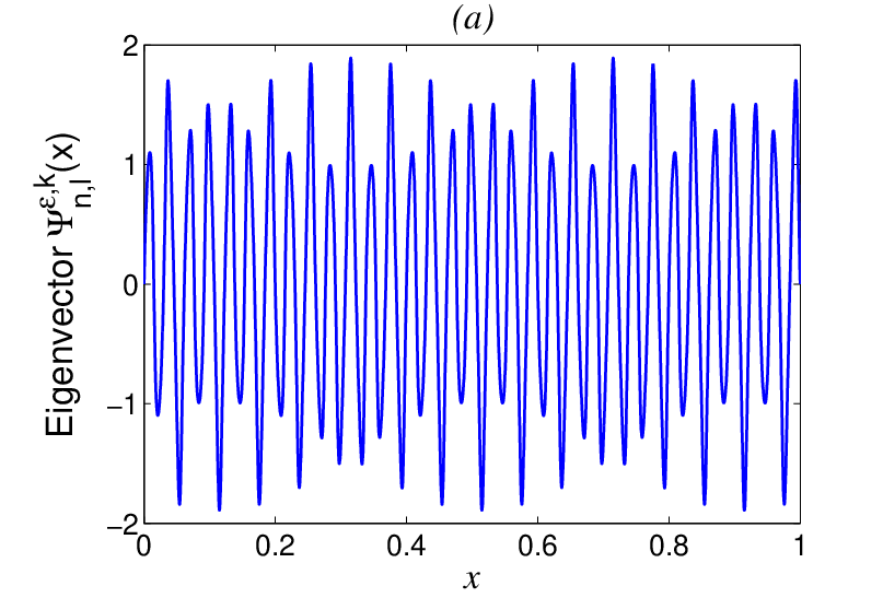
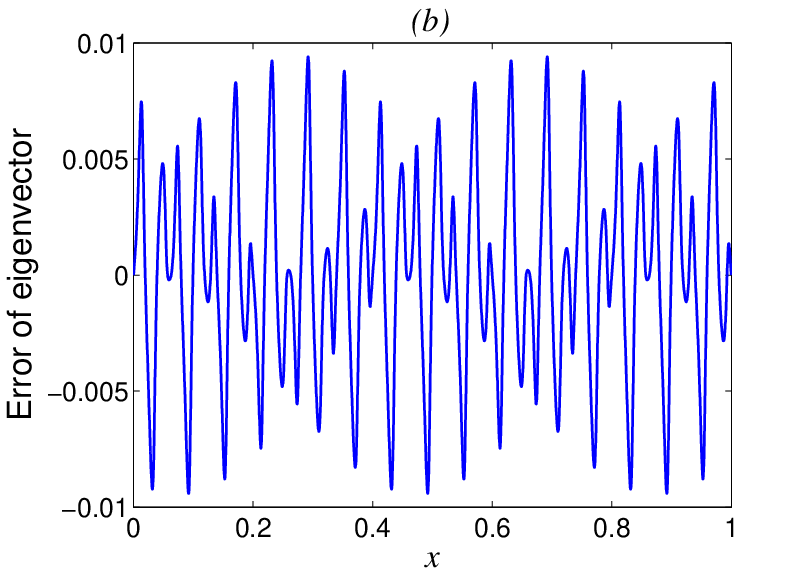
Additional results for with are reported in Figures 8 (a) and (b) showing and respectively.


6.4 Order of convergence
For a given pair and , we investigate the order of convergence of the errors and when the number of cells increases. To follow the convergence result, the sequence of periods is in fact a subsequence satisfying
with and for a sequence of . Table 3 summarizes the results for , and .
Table 3: Errors for a decreasing subsequence
To evaluate the decay rate of the errors, we pose and , so the decay rates satisfy
Using successive results for and , yields
with coefficients
References
- [1] Grégoire Allaire. Homogenization and two-scale convergence. SIAM Journal on Mathematical Analysis, 23(6):1482–1518, 1992.
- [2] Grégoire Allaire. Two-scale convergence and homogenization of periodic structures. School on homogenization, ICTP, Trieste, 1993.
- [3] Grégoire Allaire and Guillaume Bal. Homogenization of the criticality spectral equation in neutron transport. ESAIM: Mathematical Modelling and Numerical Analysis, 33(04):721–746, 1999.
- [4] Grégoire Allaire, Yves Capdeboscq, Marjolaine Puel, et al. Homogenization of a one-dimensional spectral problem for a singularly perturbed elliptic operator with neumann boundary conditions. DCDS-B, 2012.
- [5] Grégoire Allaire and Carlos Conca. Bloch-wave homogenization for a spectral problem in fluid-solid structures. Archive for rational mechanics and analysis, 135(3):197–257, 1996.
- [6] Grégoire Allaire and Carlos Conca. Bloch wave homogenization and spectral asymptotic analysis. Journal de mathématiques pures et appliquées, 77(2):153–208, 1998.
- [7] Guillaume Bal. Homogenization of a spectral equation with drift in linear transport. ESAIM: Control, Optimisation and Calculus of Variations, 6:613–627, 2001.
- [8] Matthieu Brassart and Michel Lenczner. A two-scale model for the periodic homogenization of the wave equation. Journal de mathématiques pures et appliquées, 93(5):474–517, 2010.
- [9] J Casado-Diaz. Two-scale convergence for nonlinear dirichlet problems in perforated domains. In Proceedings Section A: Mathematics-Royal Society of Edinburgh, volume 130, pages 249–276. Royal Society of Edinburgh, 2000.
- [10] Doina Cioranescu, Alain Damlamian, and Georges Griso. Periodic unfolding and homogenization. Comptes Rendus Mathematique, 335(1):99–104, 2002.
- [11] Doina Cioranescu, Alain Damlamian, and Georges Griso. The periodic unfolding method in homogenization. SIAM Journal on Mathematical Analysis, 40(4):1585–1620, 2008.
- [12] C Conca, R Orive, and M Vanninathan. Bloch approximation in homogenization on bounded domains. Asymptotic Analysis, 41(1):71–91, 2005.
- [13] C Conca, J Planchard, and M Vanninathan. Limiting behaviour of a spectral problem in fluid-solid structures. Asymptotic analysis, 6(4):365–389, 1993.
- [14] Carlos Conca, Rafael Orive, and Muthusamy Vanninathan. Bloch approximation in homogenization and applications. SIAM journal on mathematical analysis, 33(5):1166–1198, 2002.
- [15] Carlos Conca and Muthusamy Vanninathan. Homogenization of periodic structures via bloch decomposition. SIAM Journal on Applied Mathematics, 57(6):1639–1659, 1997.
- [16] M Conca and M Vanninathan. A spectral problem arising in fluid-solid structures. Computer methods in applied mechanics and engineering, 69(2):215–242, 1988.
- [17] Srinivasan Kesavan. Homogenization of elliptic eigenvalue problems: Part 1. Applied Mathematics and Optimization, 5(1):153–167, 1979.
- [18] Srinivasan Kesavan. Homogenization of elliptic eigenvalue problems: Part 2. Applied Mathematics and Optimization, 5(1):197–216, 1979.
- [19] M Lenczner. Multiscale model for atomic force microscope array mechanical behavior. Applied Physics Letters, 90(9):091908–091908, 2007.
- [20] Michel Lenczner. Homogenization of linear spatially periodic electronic circuits. Networks and Heterogeneous Media, 1:467–494, 2006.
- [21] Dag Lukkassen, Gabriel Nguetseng, and Peter Wall. Two-scale convergence. Int. J. Pure Appl. Math, 2(1):35–86, 2002.
- [22] Sergey A Nazarov, Iryna L Pankratova, and Andrey L Piatnitski. Homogenization of the spectral problem for periodic elliptic operators with sign-changing density function. Archive for rational mechanics and analysis, 200(3):747–788, 2011.
- [23] Gabriel Nguetseng. A general convergence result for a functional related to the theory of homogenization. SIAM Journal on Mathematical Analysis, 20(3):608–623, 1989.
- [24] I Pankratova and A Piatnitski. Homogenization of spectral problem for locally periodic elliptic operators with sign-changing density function. Journal of Differential Equations, 250(7):3088–3134, 2011.
- [25] M Vanninathan. Homogenization of eigenvalue problems in perforated domains. In Proceedings of the Indian Academy of Sciences-Mathematical Sciences, volume 90, pages 239–271. Springer, 1981.