Localized Pressure and equilibrium statesThanks: This work was partially supported by a grant from the Simons Foundation (#209846 to Christian Wolf).
Abstract.
We introduce the notion of localized topological pressure for continuous maps on compact metric spaces. The localized pressure of a continuous potential is computed by considering only those -separated sets whose statistical sums with respect to an -dimensional potential are ”close” to a given value . We then establish for several classes of systems and potentials and a local version of the variational principle. We also construct examples showing that the assumptions in the localized variational principle are fairly sharp. Next, we study localized equilibrium states and show that even in the case of subshifts of finite type and Hölder continuous potentials, there are several new phenomena that do not occur in the theory of classical equilibrium states. In particular, ergodic localized equilibrium states for Hölder continuous potentials are in general not unique.
Key words and phrases:
topological pressure, generalized rotation sets, variational principle, equilibrium states, thermodynamic formalism1. Introduction
1.1. Motivation
The thermodynamic formalism has been an important tool in the development of the theory of dynamical systems. Originally, this subject was primeraly driven by applications in dimension theory that followed the pioneer works carried out by Ruelle, Bowen and Manning and McCluskey [5, 28, 21]. These works inspired numerous studies and generalizations with applications far beyond the sole focus on dimension. For example, pressure can be applied to obtain information about Lyapunov exponents, dimension, multifractal spectra, or natural invariant measures. We refer to [1, 24, 27, 29] for details and further references.
The main object in the thermodynamic formalism is the topological pressure, a certain functional defined on the space of observables that encodes several important quantities of the underlying dynamical system. The relation between the topological pressure and invariant measures is established by the variational principle. Namely, if is a continuous map on a compact metric space and is a continuous potential, then the topological pressure is given by the supremum of the free energy of the invariant probability measures (see (12) for the precise statement). This result is powerful in part because it connects in a natural but unexpected way topological and statistical dynamics. Invariant probabilities maximizing free energy are called equilibrium states. The study of equilibrium states (existence, uniqueness and properties) has a long history and the results are widely spread in the literature, yet a complete understanding is still lacking today. We refer to [4, 6, 10, 17] for references and details.
Our focus in this paper is somewhat different. We introduce a localized version of the topological pressure where the localization results from using only those orbits in the computation of the pressure whose statistical averages with respect to a given -dimensional potential are close to a vector . We then establish a version of the localized variational principle for a wide variety of systems and potentials. We also show that the assumptions in our localized variational principle are fairly sharp. Finally, we develop the theory of localized equilibrium states and derive non-uniqueness results for these equilibrium states. Our results significantly distinguish localized equilibrium states from the theory of classical equilibrium states.
The results in this paper are related and can be considered in some sense extensions of results in the higher dimensional multifractal analysis developed by Barreira, Saussol, Schmeling, Takens, Verbitskiy, and others (see for example [2, 3, 30]). For localizations using restrictions of the pressure to non-compact subsets we refer to [7, 25, 31] and the references therein. We will now describe our results in more detail.
1.2. Basic definitions and statement of the results.
Let be a continuous map on a compact metric space . We consider continuous potentials and . We think of as our target potential for computing the localized topological pressure and of as the potential providing the localization. For and , we say that is -separated if for all with we have . Note that is a metric (called Bowen metric) that induces the same topology on as . For and , we denote by the -dimensional Birkhoff average at of length with respect to , where
| (1) |
and . Given and we say a set is a -set if is -separated set and for all the Birkhoff average is contained in the Euclidean ball with center and radius . We define the localized topological pressure of the potential (with respect to and ) by
| (2) |
where
| (3) |
This definition is analogous to that of the classical topological pressure with the exception that we here only consider orbits with Birkhoff averages close to . Moreover, when we omit the limit in (2) and choose large enough that the range of is contained in , then we obtain the classical topological pressure of .
Note that the definition of is only meaningful if contains statistical averages with respect to for infinitely many and arbitrarily small . We call the corresponding set of points the pointwise rotation set of and denote it by , that is
| (4) |
Next, we discuss a measure-theoretic approach to rotation sets and localized pressure. We denote by the set of all Borel -invariant probability measures on endowed with the weak∗ topology. Following [14], we define the generalized rotation set of by
| (5) |
where denotes the rotation vector of the measure . We call the rotation class of . In [18] we study the relationship between the pointwise rotation set and generalized rotation set of . In particular, we show that with strict inclusion in certain cases. We also provide criteria for the equality of the two rotation sets. We refer to the overview article [22] and to [14, 18, 33] for further details about rotation sets. For , we define the localized measure-theoretic pressure of the potential (with respect to and ) by
| (6) |
In case we take the supremum in (6) over all invariant measures we obtain the classical measure-theoretic pressure. The classical variational principle (without localization) states that the topological and the measure-theoretic versions of the pressure coincide. However, it turns out that in the case of localized pressure, the measure-theoretic and topological pressures may differ and strict inequalities can occur in both directions. This follows from the Examples 1 and 2 given in Section 3. On the other hand, the following result (see Theorem 1 in the text) gives a fairly complete description of the assumptions needed to still have a variational principle.
Theorem A.
Let be a continuous map on a compact metric space that is a Besicovitch space. Let and be continuous and let be such that the map is continuous at and is approximated by ergodic measures. Then .
The assumption that is approximated by ergodic measures (see Section 3 for the precise definition) cannot be dropped in Theorem A. Indeed, Example 1 does not satisfy this assumption and holds. On the other hand, without the assumption that is continuous at , Theorem A is in general not true, which is a consequence of Example 2. We recall that the continuity of holds for all if the entropy map is upper semi-continuous. In particular, this is true if is expansive [32], a map on a compact smooth Riemannian manifold [23] or satisfies the entropy-expansiveness (as for example certain partial hyperbolic systems [12]). Recently, there has been significant progress in finding milder conditions that imply the upper-semicontinuity of the entropy function (see for example [8]).
We note that Theorem A holds for a wide variety of systems and potentials. In particular, Theorem A holds for systems with strong thermodynamic properties (STP) (see Section 3).
Next, we present our results about localized equilibrium states. Fix . We say is a localized equilibrium state of (with respect to and ) if
| (7) |
This definition is analogous to that of a classical equilibrium state with the exception that we here only consider invariant measures in rather than all invariant measures. Evidently, the upper semi-continuity of the entropy map guarantees the existence of at least one localized equilibrium state. Unlike in the case of classical equilibrium states, there does not need to exist an ergodic localized equilibrium state (see Example 3). In Section 4 we introduce the class of systems with strong thermodynamic properties that include subshifts of finite type, hyperbolic systems and expansive homeomorphisms with specification. These systems exhibit the strongest possible properties for classical equilibrium states. In particular, for each Hölder continuous potential , there exists a unique equilibrium state (which is ergodic) and has the Gibbs property. We show that this result does not carry over to localized equilibrium states. In Example 4 we consider a shift map and construct a Lipschitz continuous potential exhibiting exactly two ergodic localized equilibrium states, none of which is Gibbs. We call the corresponding rotation set the ”fish” due its shape. We study this example in great detail and derive properties that can be used to construct further counter examples. Indeed, we are able to prove that the boundary of the fish is an infinite polygon and compute an exact formula for the corresponding vertices. By slightly modifying this example, we show that the cardinality of ergodic localized equilibrium states is in general not preserved under small perturbations of the potential. All these examples are formulated for (i.e. the localized entropy) and . In Theorem B (i) (see below), we show that these phenomena do not not occur if int .
This motivates the following definition: Let be a localized equilibrium state of (with respect to and ). We say is an interior localized equilibrium state if (where denotes the relative interior of the set), otherwise we say is a localized equilibrium state at the boundary. Without loss of generality we can always assume that (i.e. has non-empty interior ) because otherwise we could just consider a lower dimensional affine subspace. The following result shows that interior equilibrium states still share many of the properties of classical equilibrium states.
Theorem B.
Suppose that is a system with strong thermodynamic properties. Let and be Hölder continuous potentials, and let . Then
- (i)
If , then there exists a unique (ergodic) localized equilibrium state at .
- (ii)
Suppose and that all localized equilibrium states of are interior equilibrium states. Then the set of ergodic localized equilibrium states is non-empty and finite.
- (iii)
Under each of the assumptions (i) or (ii), every ergodic localized equilibrium state is a classical equilibrium state of the potential for some and .
We note that part (i) of Theorem B holds in particular for (and more generally if is cohomologous to a constant). Therefore, the assumption implies the existence of an unique localized measure of maximal entropy. Another interesting feature of Theorem B is that in both cases, (i) and (ii) the ergodic localized equilibrium state is a classical equilibrium state. This implies that if is a subshift of finite type, a uniformly hyperbolic system or an expansive homeomorphism with specification, any ergodic localized equilibrium state is a Gibbs state.
The proof of Theorem B relies heavily on methods from the thermodynamic formalism and, in particular, on the analyticity of the topological pressure for Hölder continuous potentials. Moreover, we use results of Jenkinson [14] as key ingredients.
This paper is organized as follows: In Section 2, we review some background material. Section 3 is devoted to the proof of the localized variational principle (Theorem A) and the construction of certain examples showing that without the assumptions of Theorem A, the localized variational principle fails. Finally, in Section 4 we discuss localized equilibrium states and discover fundamental differences between the theory of classical and localized equilibrium states. In particular, we prove Theorem B for systems with strong thermodynamic properties.
2. Preliminaries
In this paper we consider deterministic discrete-time dynamical systems given by a continuous map on a compact metric space . We are concerned with a continuous potential and an -dimensional continuous potential . Consider the set of all Borel -invariant probability measures endowed with weak∗ topology and denote by the subset of ergodic measures. We recall the definition of the pointwise rotation set (see (4)) and the rotation set (see (5)). Similarly, the ergodic rotation set is defined by
| (8) |
Rotation sets originated from Poincaré’s rotation numbers for circle homeomorphisms [26]. The relation between the three different rotation sets is studied in detail in [18]. Both, and are compact and is convex. We always have
| (9) |
where both inclusions can be strict. The first inclusion follows from Birkhoff’s Ergodic Theorem and the second is a consequence of the sequential compactness of (see [18] for details).
For completeness we now recall the notion of the classical topological pressure. For and let
| (10) |
The topological pressure with respect to the dynamical system is a mapping defined by
| (11) |
The topological entropy of is defined by . We simply write and if there is no confusion about . The topological pressure is real valued if and only if the topological entropy of is finite. We use as a standing assumption in this paper. The topological pressure satisfies the well-known variational principle
| (12) |
Here denotes the measure-theoretic entropy of with respect to (see [32] for details). It is a straight forward conclusion that the supremum in (12) can be replaced by the supremum taken only over all .
3. Localized Pressure
Our goal is to prove the local version of the variational principle, namely . However, in general this equality does not hold even if the potential is identically zero. The following examples show that with no additional assumptions we do not have even a one-sided inequality.
Example 1.
This is an example of a dynamical system where at certain points localized topological pressure is strictly less that the localized measure-theoretic pressure. We concatenate three non-overlapping one-dimensional dynamical systems such that the entropy of the outside components is greater than the entropy of the inside one. We take the potential to be the identity map and to be zero. Since in this case the topological pressure does not exceed the topological entropy, the affine property of the measure-theoretic pressure implies the strict inequality at the center points. What follows is the concrete construction.
Let , where , , and . We define to be the logistic type map on and given by
Then .
Whenever satisfies we will reach our conclusion. For example, take to be a Cantor set in the interval and to be a homeomorphism on the Cantor set which is topologically conjugate to a subshift whose entropy is strictly less than . One possibility is the subshift with transition matrix . We may also let and with . In this case .
We take the potential to be the identity map on . Then for any point we have since localized measure-theoretic pressure is an affine function of . However, . Therefore, .
The next example will address the reverse inequality.
Example 2.
Consider a decreasing sequence of disjoint compact intervals on the real line whose left end-points converge to . We define the function on each to be conjugate to the logistic map on and maps onto . Moreover, . Then is compact and is continuous on . Moreover, for each the interval is invariant with respect to . Since is conjugate to on , the topological entropy of is equal to the topological entropy of on and therefore is .
As an example of such construction consider disjoint dyadic intervals . In this case is defined in the following way.
Take the identity potential . Let be the entropy maximizing ergodic measures on . Then . Since , we have . However, is a fixed point of and also an extreme point of . Thus, the only invariant measure on with is the point-mass measure at zero. Therefore, .
We say that is approximated by ergodic measures at if there exists such that and as . In this case we have . Indeed, for there exists such that . The ergodicity of implies the existence of such that for arbitrary large . Therefore, and thus .
We say that a metric space is Besicovitch if the Besicovitch covering theorem holds (see [11, 20]). The next theorem is a local version of the variational principle.
Theorem 1.
Let be a continuous map on a compact metric space that is a Besicovitch space. Let and be continuous and let such that the map is continuous at and is approximated by ergodic measures. Then .
Proof.
We first show that . Fix . It follows from the definition of and the continuity of that there exist and such that
| (13) |
and for any we have
| (14) |
We will now apply the method of constructing measures with large free energies which is commonly used to prove the classical variational principle. Let be separated sets in such that for all and Let be the atomic measure concentrated on given by the formula
| (15) |
where denotes the Dirac measure supported on . Consider a sequence of measures and let be a weak∗ accumulation point of . Then (see [32] or [16, Section 4.5]) is -invariant and satisfies
| (16) |
We conclude that
| (17) | ||||
Note that by the construction of . Therefore, . Since was arbitrary, we obtain the desired inequality .
Now we turn our attention to the opposite inequality. Let be arbitrary. As before, we fix and such that for any
| (18) |
Since is uniformly continuous on we may assume that is chosen small enough so that for any and with we have
| (19) |
Since is approximated by ergodic measures, there exists such that
| (20) |
There is a generalization of Katok’s characterization of the measure-theoretic entropy in terms of ergodic measures to the concept of topological pressure derived in [13]. See [15] for the original approach. We are using the following set up: Fix . We say that is an -spanning set for if . Denote by , where the infimum is taken over all -spanning sets of a set of -measure more than or equal to . Then
| (21) |
There exists a decreasing sequence of strictly positive numbers with and corresponding sequences of -spanning sets such that
| (22) |
and
| (23) |
We may assume that each is a minimal spanning set with respect to the inclusion. Since is ergodic, the basin of defined by
| (24) |
is a set of full -measure by Birkhoff’s Ergodic Theorem. We define
| (25) |
Since is an increasing sequence of Borel sets whose union is a set of full -measure, we conclude that . Consider the sequence of sets
| (26) |
It follows from (19) and (20) that for any we have . When is sufficiently large, is a spanning set for a set of -measure greater than where . Therefore,
| (27) |
It follows from the fact that (21) also holds for that for small enough (23) remains true when we replace by .
Let be a Besicovitch constant of . Note that this constant can be chosen independently of the metrics since they are decreasing in . It follows from the Besicovitch covering theorem and the fact that is minimal that where each is an -separated set. We conclude that
| (28) |
Combining inequality (28) with (18), (20) and (23) we obtain
| (29) |
Since was arbitrary, this concludes the proof of the theorem. ∎
Note that the left hand side inequality between the topological and measure-theoretic localized pressures was proven under milder assumptions. More precisely, we have the following.
Corollary 1.
Let be a continuous map on a compact metric space , let and be continuous and let such that the map is continuous at . Then .
4. equilibrium states
Let be a continuous map on a compact metric space and let . Fix . We recall the definition of being a localized equilibrium state of with respect to and in (7).
We say that the entropy map is upper semi-continuous at if for every with and every accumulation point of we have . Note that if the entropy map is upper semi-continuous at then there exists for each at least one localized equilibrium state of . The following example shows that the existence of a localized equilibrium state does in general not imply the existence of an ergodic localized equilibrium state. This differs from the theory of classical equilibrium states where the existence of an equilibrium state always guarantees the existence of an ergodic equilibrium state (see [32]).
Example 3.
Let with . Let and be a continuous transformation with an upper semi-continuous entropy map such that and . Moreover, we assume that , , and . Consider the potentials and . Since the convexity of implies . Any can be written as , where and are ergodic entropy maximizing measures on and respectively. It follows that the measure is a localized equilibrium state of with respect to and . However, the set does not contain any ergodic measure.
We will see that even in the case of systems satisfying the strongest possible existence and uniqueness results for classical equilibrium states the situation for localized equilibrium states is rather different. We now introduce the class of systems with strong thermodynamic properties.
4.1. Systems with strong thermodynamic properties
We say has strong thermodynamic properties (which we abbreviate by (STP)) if the following conditions hold:
- 1.
;
- 2.
The entropy map is upper semi-continuous;
- 3.
The map is real-analytic on ;
- 4.
Each potential has a unique equilibrium measure such that . Furthermore, is ergodic and given we have
(30) - 5.
For each , we have if and only if is cohomologous to a constant.
- 6.
For each , and we have
(31) with equality if and only if is cohomologous to a constant.
Note that for several classes of systems properties (3)-(6) hold even for a wider class of potentials, namely for potentials with summable variation (see for example [14]). For simplicity, we restrict our considerations to Hölder continuous potentials.
Some examples of systems with strong thermodynamic properties are expansive homeomorphisms with specification which include topological mixing two-sided subshifts of finite type as well as diffeomorphisms with a locally maximal topological mixing hyperbolic set, see [6, 10, 16, 29]. We note that in all these examples the measure in property (4) is a Gibbs measure. Next, we introduce some concepts about shift maps that will be used later on.
Let and let be a finite alphabet in symbols. The (one-sided) shift space on the alphabet is the set of all sequences where for all . We endow with the Tychonov product topology which makes a compact metrizable space. For example, given it is easy to see that
| (32) |
defines a metric which induces the Tychonov product topology on . The shift map (defined by ) is a continuous to map on . If is an -invariant set we say that is a sub-shift. In particular, for a matrix with values in we define . It is easy to see that is a closed (and therefore compact) -invariant set and we say that is a subshift of finite type. A subshift of finite type is (topologically) mixing if is aperiodic, that is, if there exists such that for all .
Analogously, we obtain the concept of two-sided shift spaces and shift maps by defining to be the space of all bi-infinite sequences where for all . It is a well-known fact that topological mixing sub-shifts of finite type have strong thermodynamic properties (see [29]).
4.2. Interior and boundary equilibrium states
From now on we assume that has strong thermodynamic properties, and . Recall that if is Hölder continuous then is equivalent to the condition that no non-trivial linear combination is cohomologous to a constant. For we define the relative interior of (denoted by ) as the interior of considered as a subset of the smallest affine subspace of containing . In particular, if has non-empty interior then the relative interior and the interior of coincide.
Definition 1.
Suppose is a localized equilibrium state of with respect to and . We say that is an interior equilibrium state if . Otherwise, call a localized equilibrium state at the boundary.
We note that if and only if either is cohomolous to a constant or is cohomologous to some nontrivial linear combination of . In this situation we say that a localized equilibrium state of with respect to and is a localized measure of maximal entropy at .
The following example shows that localized equilibrium states at the boundary are in general not unique.
Example 4.
Let be the one-sided full shift with alphabet . Let be a compact and convex subset of whose boundary is a strictly convex Jordan curve. Pick any point . Then there exists a line passing through which does not intersect , but its orthogonal line does. Let be any point in on that orthogonal line and let be points on on opposite sides with respect to the line. Denote by the arcs in joining and . For we pick a strictly unidirectional sequence starting at and going towards . We require that and for all , in particular .
Next, we define several subsets of .
Let and fix .
For and all we define . Moreover, let .
Finally, we define a potential by
| (33) |
Note that if and only if either for all or for all , in particular is a subshift finite type with transition matrix
| (34) |
To illustrate this example we consider a case where the set and the sets of points , are symmetric about the line through and . We denote by the rotation vectors of the periodic orbits of length whose generators have the first coordinates in and the coordinate in the complementary alphabet . Precisely, for and we have
| (35) |
We show that in this case the boundary of is the infinite polygon. Moreover, there is a neighborhood of where the vertices of are exactly , and for some integer which depends on properties . We prove this fact in the next proposition by introducing a new coordinate system with the origin at and and the -axis passing through . For a given point we write and for the and coordinates respectively. Let denote the parametrized boundary curve of the upper half of . By symmetry coincides with the boundary curve of the lower half. For simplicity we add an additional assumption on that guaranties that .
Proposition 1.
Proof.
First we show that the sequence of points is monotonically decreases to the origin. By symmetry, this immediately implies that the sequence increases monotonically to the origin. It follows from (35) that for any we have
| (37) |
The -coordinate of is always positive, since the are decreasing and . The -coordinate of simplifies to
| (38) |
This expression is positive whenever . This can always be achieved starting from some since is decreasing to zero. Therefore, are decreasing for . The assumptions of the proposition assure that we may take , however this condition is not essential.
The result by Sigmund that the periodic point measures are dense in reduces our considerations to rotation vectors of periodic orbits.
Suppose is a periodic point of period . We may assume that and is maximally partitioned into blocks of sizes such that , and each block exclusively contains elements of either or . It follows from the construction of that (where denotes the rotation vector of the unique invariant measure supported on the orbit of ) is the sum of blocks of vectors of the form
| (39) |
Here if the elements of block are from and if the elements of block are from . In case the block’s contribution is .
First we show that for . In this case we have
| (40) |
By symmetry we restrict ourselves to the case . We compare with points and . For the -coordinates we obtain that
| (41) |
as long as for either or . When we obtain , which is the mid-point between and . For the -coordinates we obtain
| (42) |
and thus .
The case is similar. We have with . By symmetry, we may assume that is above the -axis and that we can write
| (43) |
We compare with points and . For the -coordinates we obtain
| (44) |
whenever for at least for one . In the case we have .
For the -coordinates we see that
| (45) |
It follows that .
To conclude the proof we notice that the rotation vector of any periodic orbit can be written as a convex combination of vectors described in the previous two cases and . ∎
Figure 1 illustrates the rotation set of the potential (see (33)) where the set is a ellipse , , for and . Below we plot 1000 data points of this rotation set. The shape of the resulting graph gives it the name ’fish’.
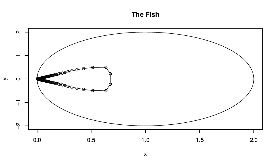
We now list several properties of the system in Example 4 that hold without the symmetry assumptions in Proposition 1.
Theorem 2.
Let and be as in Example 4. Then
- (i)
is Lipschitz continuous;
- (ii)
and ;
- (iii)
There exists precisely two ergodic localized measures of maximal entropy at ;
- (iv)
The entropy function is real analytic in .
Proof.
(i) We will work with the metric (see (32)) on to show that is Lipschitz continuous. Set . Let with . If then for some . Hence,
| (46) |
The case is analogous. The case and with can be treated analogously as in (46). It remains to consider the case for some . Without loss of generality we assume that is further along on the path to as . Thus, where is defined by . Since for all , we conclude that
| (47) |
which completes the proof of (i).
(ii) Note that points and belong to and thus .
To prove that we apply again the result of Sigmund that the periodic point measures are weak∗ dense in . Suppose is a periodic point of period and that we have the decomposition (39). We use the notation
| (48) |
Then the rotation vector of any periodic orbit can be written as a convex combination of and . The fact that the set is strictly convex implies that for all . Also, it is easy to see that the converge to as . Indeed,
| (49) | ||||
Since and is their only accumulation point, we have and thus .
(iii) We will compute the logarithmic rate of growth of periodic orbits with rotation vectors in the neighborhood of . Fix . Suppose is a periodic point of period and . We may assume decomposition (39). Since there are blocks and each block contributes at least one to we have
| (50) |
Therefore, . Denote , the largest integer smaller than . Note that since .
The maximal number of points of period in is
| (51) |
We will estimate . We have
| (52) | ||||
In the last equality we used the sum of geometric progression with common ratio which is less than one since . We obtain
| (53) |
Using the well known fact that we obtain
| (54) |
To simplify the notation in the following computation we denote . Using , we estimate the growth rate of the periodic orbits of period in .
| (55) |
Passing to the limit as approaches infinity we obtain the growth rate of the periodic orbits
| (56) | ||||
Note that the last expression is greater than since . Since as , we have
| (57) |
Therefore, we have . Thus, the two distinct ergodic localized measures of maximal entropy at are the two ergodic measures of maximal entopy of .
Finally, (vi) is a result of [18].
∎
Remarks.
(i) The cardinality of ergodic localized equilibrium states at the boundary is in general not preserved under small changes of the potential . Indeed, for any pick a point such that and dist. Redefine within an -neighbourhood so that . Define
| (58) |
Clearly . However, has a unique (ergodic) localized measure of maximal entropy at and has precisely two ergodic localized measures of maximal entropy at .
(ii) In a forthcoming note we construct examples of Hölder continuous potentials with countable infinitely many ergodic localized equilibrium states at some boundary point of . We refer to [19] for details.
Next, we consider interior localized equilibrium states. Recall our standing assumptions that for some and that (i.e. no non-trivial linear combination is cohomologous to a constant). Let . We first consider the case . As noted before, this means that either is cohomologous to a constant or is cohomologous to some non-trivial linear combination . It follows from the convexity of that is a singleton. In particular, is a localized equilibrium state of with respect to and if and only if is a localized measure of maximal entropy at . For let us denote by the (classical) equilibrium state of the potential (which is well-defined by property 4 of (STP)). In [18] we proved the following result.
Theorem 3.
Let and assume is a singleton. Then there exits a unique localized measure of maximal entropy at . Moreover, for some uniquely defined .
We now consider the case . Let . It follows from the compactness and the convexity of that there exist such that
| (59) |
For let denote the uniquely defined (classical) equilibrium measure of the potential . In [18] we showed that the map defined by
| (60) |
is a real-analytic diffeomorphism and that is the unique measure satisfying
| (61) |
Moreover, the map is real-analytic. For we write .
Proposition 2.
Let . Then the map is a real-analytic diffeomorphism onto its image and is the unique measure satisfying
| (62) |
In particular, if is an interior ergodic localized equilibrium state of with respect to and , then there exists a unique with .
Finally, we present our main result about interior localized equilibrium states.
Theorem 4.
Supose that all localized equilibrium states of with respect to and are interior equilibrium states. Then there exists at least one and at most finitely many ergodic localized equilibrium states of with respect to and . All these ergodic localized equilibrium states are classical equilibrium states.
Proof.
Since there exists a localized equilibrium state of , we may conclude from Proposition 2 the existence of an ergodic localized equilibrium state of with respect to and . Suppose there exist infinitely many ergodic localized equilibrium states of . Again by Proposition 2 there exists a pairwise disjoint sequence such that each is an ergodic localized equilibrium state of . Let be a weak∗ accumulation point of the measures . It follows that is also a localized equilibrium state of . Recall that there are no localized equilibrium states at the boundary Thus, Proposition 2 implies that for some . We conclude that the function is constant on a non-discrete subset of . Hence, is constant by the identity theorem. Thus, is a localized equilibrium state of with respect to and for every . But this implies that there must exist a localized equilibrium state of with respect to and at the boundary which is a contradiction.
∎
References
- [1] L. Barreira and K. Gelfert, Dimension estimates in smooth dynamics: a survey of recent results, Ergodic Theory and Dynamical Systems 31 (2011), 641–-671.
- [2] L. Barreira, B. Saussol and J. Schmeling Higher-dimensional multifractal analysis, J. Math. Pures Appl. 9 (2002), 67–-91.
- [3] L. Barreira and B. Saussol, Variational principles and mixed multifractal spectra, Trans. Amer. Math. Soc. 353 (2001), 3919–-3944.
- [4] R. Bowen, Equilibrium states and the ergodic theory of Anosov diffeomorphisms, Lecture Notes in Math. 470, Springer-Verlag, Berlin, 1975.
- [5] R. Bowen, Hausdorff dimension of quasicircles, Inst. Hautes Études Sci. Publ. Math. 50 (1979), 11–25.
- [6] R. Bowen, Some systems with unique equilibrium states, Math. Systems Theory 8 (1974/75), 193–-202.
- [7] V. Climenhaga Topological pressure of simultaneous level sets, Nonlinearity 26, (2013), 241–-268.
- [8] V. Climenhaga and Thompson, Equilibrium states beyond specification and the Bowen property, Journal London Mathematical Society (2) 87 (2013), 401–-427.
- [9] M. Denker, C. Grillenberger and- K. Sigmund, Ergodic theory on compact spaces, Lecture Notes in Mathematics, Vol. 527. Springer-Verlag, Berlin-New York, 1976. iv+360 pp.
- [10] N. Haydn and D. Ruelle, Equivalence of Gibbs and equilibrium states for homeomorphisms satisfying expansiveness and specification, Comm. Math. Phys. 148 (1992), 155–-167.
- [11] H. Federer, Geometric measure theory, Springer-Verlag Berlin Heidelberg New York, 1996.
- [12] T. Fisher, L. Diaz, M. Pacifico and J. Vieitez, Entropy-expansiveness for partially hyperbolic diffeomorphisms, Discrete Contin. Dyn. Syst. 32 (2012), 4195–-4207.
- [13] L. He, J. Lv and L. Zhou, Definition of measure-theoretic pressure using spanning sets, Acta Math. Sinica, English series 20 (2004), 709–718.
- [14] O. Jenkinson, Rotation, entropy, and equilibrium states, Trans. Amer. Math. Soc. 353 (2001), 3713–3739.
- [15] A. Katok, Lyapunov exponents, entropy and periodic orbits for diffeomorphisms, Publ. Math., Inst. Hautes Étud. Sci. 51 (1980), 137–173.
- [16] A. Katok and B. Hasselblatt, Introduction to the modern theory of dynamical systems. With a supplementary chapter by Katok and Leonardo Mendoza, Encyclopedia of Mathematics and its Applications, 54, Cambridge University Press, Cambridge, 1995.
- [17] G. Keller, Equilibrium states in ergodic theory, London Mathematical Society Student Texts, 42, Cambridge University Press, Cambridge, 1998. x+178 pp.
- [18] T. Kucherenko and C. Wolf, Geometry and entropy of generalized rotation sets, Israel Journal of Mathematics, to appear.
- [19] T. Kucherenko and C. Wolf, On finitelness of localized equilibrium states, in preparation.
- [20] P. Loeb, On the Besicovitch covering theorem, SUT J. Math. 25 (1989), 51-–55.
- [21] A. Manning and H. McCluskey, Hausdorff dimension for horseshoes, Ergodic Theory Dynamical Systems 3 (1983), 251–260.
- [22] M. Misiurewicz, Rotation Theory, Misiurewicz’s webpage.
- [23] S. Newhouse, Continuity properties of entropy, Ann. of Math. (2) 129 (1989), 215–235.
- [24] Y. Pesin, Dimension Theory in Dynamical Systems: Contemporary Views and Applications, Chicago Lectures in Mathematics, Chicago University Press, Chicago, 1997.
- [25] Ya. Pesin and B. Pitskelʹ, Topological pressure and the variational principle for noncompact sets, (Russian) Funktsional. Anal. i Prilozhen. 18 (1984), 50–-63.
- [26] H. Poincaré, Sur les cousbes définies par les équations différentielles, Euvres Complètes, tome 1, Gauthier-Villars, Paris, (1952), 137-158.
- [27] F. Przytycki and M. Urbanski, Conformal fractals: ergodic theory methods, London Mathematical Society Lecture Note Series, 371. Cambridge University Press, Cambridge, 2010. x+354 pp.
- [28] D. Ruelle, Repellers for Real Analytic Maps, Ergodic Theory and Dynamical Systems 2 (1982), 99–107.
- [29] D. Ruelle, Thermodynamic Formalism, Cambridge: Cambridge Univ. Press, 2004.
- [30] F. Takens and E. Verbitskiy, On the variational principle for the topological entropy of certain non-compact sets, Ergodic Theory Dynam. Systems 23 (2003), 317–-348.
- [31] D. Thompson, A thermodynamic definition of topological pressure for non-compact sets, Ergodic Theory and Dynamical Systems 31 (2011), 527–547.
- [32] P. Walters, An introduction to ergodic theory, Graduate Texts in Mathematics 79, Springer, 1981.
- [33] K. Ziemian, Rotation sets for subshifts of finite type, Fund. Math. 146 (1995), 189–201.