Learning User-specific Latent Influence and
Susceptibility from
Information Cascades
Abstract
Predicting cascade dynamics has important implications for understanding information propagation and launching viral marketing. Previous works mainly adopt a pair-wise manner, modeling the propagation probability between pairs of users using independent parameters for users. Consequently, these models suffer from severe overfitting problem, especially for pairs of users without direct interactions, limiting their prediction accuracy. Here we propose to model the cascade dynamics by learning two low-dimensional user-specific vectors from observed cascades, capturing their influence and susceptibility respectively. This model requires much less parameters and thus could combat overfitting problem. Moreover, this model could naturally model context-dependent factors like cumulative effect in information propagation. Extensive experiments on synthetic dataset and a large-scale microblogging dataset demonstrate that this model outperforms the existing pair-wise models at predicting cascade dynamics, cascade size, and “who will be retweeted”.
Introduction
Social media is revolutionizing the dissemination of information via its great ease in information delivery, accessing and filtering. In social media, users could post original messages or forward messages that they see from other users. Information propagation proceeds along social relationships between users, explicit or implicit, forming cascade dynamics. Modeling and predicting the cascade dynamics has important implications to understanding information propagation and launching viral marketing in social media. The key for this problem is inferring the interpersonal influence between users or estimating the probability that information propagates between them, fundamental to influence maximization [\citeauthoryearKempe, Kleinberg, and Tardos2003, \citeauthoryearChen, Wang, and Yang2009, \citeauthoryearCheng et al.2013], social recommendation [\citeauthoryearHuang et al.2012, \citeauthoryearMa, King, and Lyu2009], and viral marketing [\citeauthoryearRichardson and Domingos2002, \citeauthoryearLeskovec, Adamic, and Huberman2007].
Existing studies mainly aim to determine the propagation probability of information between all pairs of users, based on structure of social network, the record of information cascade, and demographic/content characteristics of users. Kempe et al. [\citeauthoryearKempe, Kleinberg, and Tardos2003] implemented the independent cascade model for information propagation, assuming a uniform propagation probability or a degree-modulated propagation probability. Goyal et al. [\citeauthoryearGoyal, Bonchi, and Lakshmanan2010] provided two static models in terms of Bernoulli distribution and Jaccard index, and learned temporal factors to maximize likelihood of cascades. Saito et al. [\citeauthoryearSaito, Nakano, and Kimura2008] learned the propagation probability for independent cascade model in terms of expectation maximization of cascades. Artzi et al. [\citeauthoryearArtzi, Pantel, and Gamon2012] estimated the propagation probability by exploiting demographic and content characteristics. These methods all adopt a pair-wise manner, modeling the propagation probability between pairs of users using independent parameters for users. Consequently, these models suffer from severe overfitting problem, limiting their prediction accuracy. For example, for a pair of users without observed interactions, these methods take the propagation probability between them as zero, indicating that it is never happened to propagate information between the two users in the future. To the best of our knowledge, we lack a model that could concisely model the interpersonal influence and accurately predict the cascade dynamics in large-scale social networks.
In this paper, we propose to model the cascade dynamics by learning two low-dimensional latent vectors for each user from observed cascades, capturing her influence and susceptibility respectively. In this latent influence and susceptibility (LIS) model, the propagation probability that one user forwards a piece of information is determined by the product of her activated neighbors’ influence vectors and her own susceptibility vector. The benefits of this model are three-fold: (1) It directly models user-specific influence and susceptibility, instead of the interpersonal influence between all pairs of users. Thus it requires much less parameters, and pairs of users are no longer independent, effectively combating the overfitting problem for pairs of users without direct interactions; (2) It could naturally capture context-dependent factors like cumulative effect in information propagation. For a target user, context means her previous exposures to the same message. In this model, one user’s previous exposures to a message improve the probability that she propagates the message, flexibly combining the benefits of both cascade model and threshold model; (3) It is applicable to scenarios with explicit or implicit social networks, since it learns user-specific influence and susceptibility from the observed information cascades rather than the underlying social networks like many existing methods.
We evaluate the proposed LIS model by extensive experiments on synthetic dataset and a large-scale microblogging dataset from Sina Weibo, the largest social media in China. Compared with several widely-used methods that work in pair-wise manner, LIS model consistently outperforms them at predicting the dynamics of cascades. Moreover, the learned user-specific influence and susceptibility vectors provide us a quantitative way to understand topic-related interpersonal influence in information propagation.
Problem formulation
In this paper, we focus on the problem of inferring users’ influence and susceptibility from detailed records of message cascades. Before diving into the details of the proposed model, we first clarify the two main motivations underlying our model.
First, existing models suffer from severe overfitting problem, especially for the pair of users without direct interactions. As shown in Fig. 1(a), when messages are forwarded by users along social links among them, not all social links matter in these message cascades. For example, no forwarding behavior occurs between users and , although they have direct social link. In this case, existing models take the propagation probability between them as zero, implying that it is never happened to propagate information between the two users in the future. This overfitting problem is actually caused by the hypothesis of existing models: interpersonal influence between different pairs of users is independent of each other. This motivates us to adopt a user-specific manner for modeling interpersonal influence among users, whose existence has been proved in [\citeauthoryearAral and Walker2012, \citeauthoryearAral, Muchnik, and Sundararajan2009]. Specifically, each user is modeled by two non-negative -dimensional vectors: an influence vector and a susceptibility vector , characterizing the influence and susceptibility of user over latent topics. For a pair of user , the interpersonal influence of on could be simply computed by the scalar product of and . This concise representation requires only parameters for users.
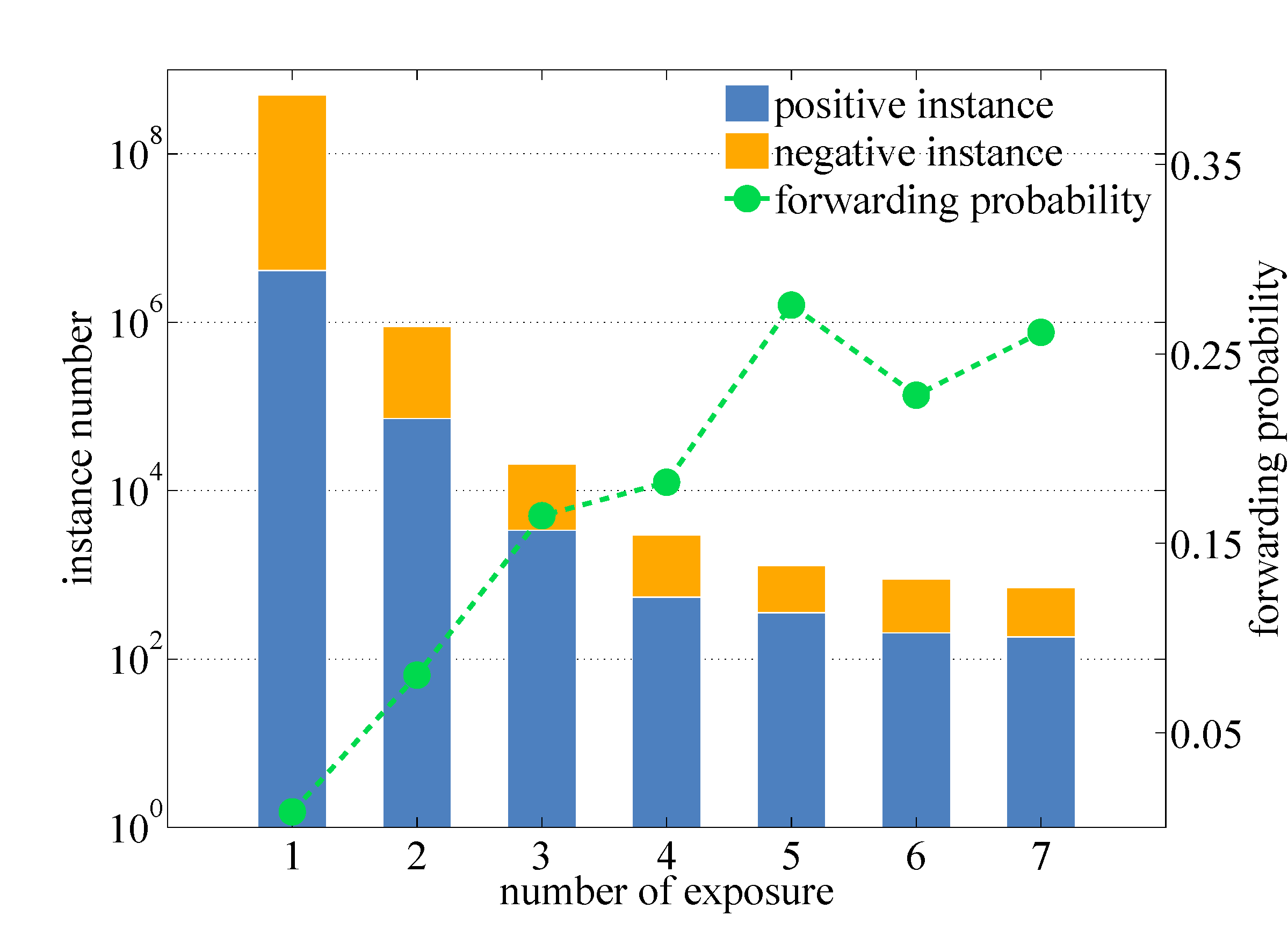
Second, the role of context in information propagation is rarely captured. Existing models mostly assume that users are memoryless, i.e., whether a user forwards one message is not affected by her previous exposures to the message. Indeed, this assumption is not supported by empirical observations from real cascades of messages. Fig. 1(b) depicts the relationship between the number of times that one user is exposed to a message and the probability that the user will forward the message when she is exposed to the message for the -th time. As the number of exposures increases, the forwarding probability increases accordingly: from 0.008 when the number of exposures is 1 to 0.261 when the number of exposures is 5. This observation clearly demonstrates that cumulative effect does exist in information propagation, an effect also observed in many other scenarios [\citeauthoryearBao et al.2013a, \citeauthoryearLeskovec, Adamic, and Huberman2007]. This motivates us to adopt a context-dependent way to model the cumulative effect.

Given a message , we denote its cascade with a chronological list of activated users , where users are ranked in the ascending order of the time they forward the message . Whenever one user is activated (i.e., she posts or forwards the message), she has one chance to attempt to activate other users. Whether her attempt succeeds depends on the cascade context at that time.
Cascade context: When one user () becomes activated and she attempts to activate a user , the cascade context for this attempt is defined as
| (1) |
where the indicator function means whether could be exposed to the message from . In other words, cascade context means ’s previous exposures to the message from other users.
In practice, it is difficult to exactly determine since there is no reliable mechanism to know whether user is exposed to a message forwarded by user , even when direct social link exists between them. In this paper, we circumvent this problem using a delegate of the function , i.e., the aggregate diffusion network of historical cascades of messages. Detailed discussions about diffusion network are given in experiments on real dataset. Diffusion network characterizes the actual flow of information between users in the past, providing us a good approximation for potential information propagation in the future. More importantly, diffusion network is always embedded in the collection of message cascades while social network is not explicitly available in many scenarios. Therefore, the proposed model is generally applicable to the scenarios with or without explicit social network.
With the above notations, we now model cascade dynamics of messages. For a message with the cascade , each user could be denoted by an -dimensional status vector , with its element indicating whether the user is in activated status right after she is exposed to the message from user . If user becomes activated when she is exposed to the message from user , we have and . If keeps inactivated during the cascade dynamics of message , for any .
The likelihood of is written as
| (2) |
where is introduced only for simplifying the notation. Here the first term depicts whether is the source of message , defined as
| (3) |
The second term characterizes the transition of user’s status, formally defined as
| (4) | ||||
where is a scaling factor, modulating the effect of cascade context. The first equation implies that a user cannot become inactivated as long as she is activated. The other two equations model how the transition probability is influenced by cascade context, reflected by a cumulative manner of interpersonal influence. The factor determines whether the user could be exposed to the message from user . For clarity, we give a graphical model representation in Fig. 2 to illustrate the process that user ’s status changes with the dynamics of message .
Assuming independent cascades, the likelihood of all cascades is a product of the likelihoods given by Eq. (2)
| (5) |

The parameters of the model are learned by minimizing the negative logarithmic likelihood, namely loss function, of all the collection of cascades as the following objective function
| (6) |
Note that is always 1, hence omitted in Eq. (6).
Parameter estimation
In this section, we develop algorithm to estimate the parameters of the proposed model. Generally speaking, parameter estimation could be completed via directly minimizing Eq. (6) with respect to and . However, the huge number of possible configurations of cascade contexts in Eq. (6) results in high computational cost. Indeed, one cascade context could repeatedly occur in many cascades, causing huge duplicated computation of Eq. (4).
Here we propose to reduce the duplicated computation by taking advantage of overlapped cascade contexts among multiple cascades. Firstly, we introduce some symbols to simplify the optimization. Let be the set of possible configurations of cascade contexts pertaining to , occurred in all cascades. For example, as shown in Fig. 1(a), , and are all the cascade contexts for user . We group cascade contexts in terms of users and re-organize the logarithmic likelihood in Eq. (6) as
|
|
(7) |
where refers to one configuration of cascade context for user , independent of specific cascade, and counts the frequency of the configuration emerged in all cascades, relative to user ’s status .
Parameters estimated by directly minimizing the logarithmic likelihood in Eq. (7) may suffer from overfitting problem, a common problem in likelihood maximization estimation. To combat this problem, we regularize the parameter vectors and and obtain the final objective function for parameter estimation
|
|
(8) |
where and are regularization parameters, and is Frobenius norm.
Finally, using Projected Gradient (PG) method [\citeauthoryearLin2007], we develop an iterative algorithm for parameter estimation, leveraging the gradients with respect to and as
|
|
(9) |
where is an indicator function, and is a concise form of . The algorithm for parameter estimation is described in Algorithm 1.
Experiments
We evaluate LIS model on both synthetic data and real world data, i.e. microblogging data from Sina Weibo. Here we only choose scalable modeling methods as baselines, i.e., expectation maximization estimation (EM) [\citeauthoryearSaito, Nakano, and Kimura2008], static Bernoulli model (SB), and static Jaccard model (SJ) [\citeauthoryearGoyal, Bonchi, and Lakshmanan2010]. To reduce the overfitting problem suffered from these models, we apply matrix factorization (MF) method [\citeauthoryearSalakhutdinov and Mnih2008] as a post-processing improvement, forming a stronger baseline. We demonstrate the benefit of the LIS model at predicting the cascade dynamics, cascade size, and “who will be retweeted”. Finally, we analyze the topics associated with the learned user-specific latent influence and susceptibility.
Experiments on synthetic data
To validate whether the proposed algorithm could obtain good estimation of user-specific influence and susceptibility, we first conduct tests on synthetic data, where cascades are generated according to parameters known a prior. These tests also offer us some intuitions about difficulties at predicting cascade dynamics.
Experimental setup.
We first generate two synthetic diffusion networks: one is constructed using Barabási-Albert (BA) model [\citeauthoryearBarabási and Albert1999], denoted as original network; the other is generated by shuffling the original network [\citeauthoryearMolloy and Reed1995], denoted as shuffle network. We set the dimensionality of user’s influence and susceptibility as 5, and sample and from , where refers to a uniform distribution. We then generate cascades over the two networks according to our LIS model with . We take 80% of the cascades generated from original network as training dataset, and the rest of cascades generated from the original network and the cascades from the shuffle network as test dataset. The two test datasets have equal size, offering a fair comparison.
Predicting cascade dynamics.
We deal with this problem as a set of binary classification problem, predicting whether one user will be activated under specific cascade context. Thus we use AUC (the area of under the ROC curve) as the evaluation metric [\citeauthoryearFawcett2006]. As a reference for the performance comparison, we offer an upper bound of our LIS model (denoted as UB): predicting cascade dynamics according to the parameters and that are used to generate cascades in test data.
Results are listed in Table 1. It is seen that LIS model consistently outperforms baselines, and its AUC value is very close to UB, when predicting on original network. Particularly, the performance of LIS model is stable on both original and shuffle networks, while baseline methods suffer from much performance reduction (some even close to 0.5, equal to random guess approach), resulted from the overfitting problem of pair-wise models.
| network | UB | LIS | SB | SJ | EM |
|---|---|---|---|---|---|
| original | 0.659 | 0.654 | 0.607 | 0.618 | 0.561 |
| shuffle | 0.659 | 0.608 | 0.509 | 0.525 | 0.507 |
Experiments on Microblog
Dataset.
The Microblog data from Sina Weibo website is published by WISE 2012 Challenge11 1 http://www.wise2012.cs.ucy.ac.cy/challenge.html, spanning from January 1, 2011 to Feburary 15, 2011. We extract the cascade records posted between January 1, 2011 and February 15, 2011, and split the extracted records into three training datasets, i.e., D1, D2, D3, each persisting a period of half a month. Furthermore, for each training dataset, we extract the cascade records in the following 5 days as test, i.e., T1, T2 and T3. We only consider the users who appear in all the three training datasets, obtaining 199,408 users. Dataset statistics are depicted in Table 2. We conduct an empirical study to demonstrate the severity of overfitting problem. Over 70% of forwarding traces—historical paths for information flows—in test data are never observed in training data, posing a big challenge to previous pair-wise models, when applied in real data.
| training data | test data | ||||
|---|---|---|---|---|---|
| cascades | period | cascades | period | ||
| D1 | 395,852 | 01/01-01/15 | T1 | 160,868 | 01/16-01/20 |
| D2 | 453,356 | 01/16-01/31 | T2 | 122,509 | 02/01-02/05 |
| D3 | 386,152 | 02/01-02/15 | T3 | 145,143 | 02/16-02/20 |
Diffusion network.
Exact diffusion network is hard to obtain, since there is no clear clues indicating whether a user is exposed to a message forwarded by her followee. Previous works focus on directly inferring diffusion networks, which is not applicable to large-scale scenarios [\citeauthoryearGomez-Rodriguez, Leskovec, and Krause2010, \citeauthoryearGomez-Rodriguez, Leskovec, and Schölkopf2013, \citeauthoryearDu et al.2012, \citeauthoryearKurashima et al.2014]. Here we estimate diffusion network according to a large collection of historical cascades: one cascade has a collection of forwarding traces over the period of observation, forming a directed graph. We aggregate these graphs of all cascades into a diffusion network, providing us a good approximation for potential information propagation in the future. Figure 3 gives an example to illustrate the construction of diffusion network.


Predicting cascade dynamics.
We introduce the length of cascade context to capture user’s context-dependent level for exploring context-dependent factors like cumulative effects in information propagation. When a user decides whether or not to forward a message, only the recent exposures take effects in cascade context. The case implies that users are memoryless, i.e., without cumulative effect, reproducing the independent assumption [\citeauthoryearKempe, Kleinberg, and Tardos2003]. To illustrate the difference of prediction performance at combating overfitting problem, we additionally evaluate the prediction only over observed forwarding traces. The experimental results are presented in Fig. 4. Despite that baselines can better handle prediction instances over observed forwarding traces, the AUCs decrease dramatically when applied to the prediction over all forwarding traces in test data. It means that pair-wise models, even with an improvement using matrix factorization, still suffer from overfitting problem when a large proportion of forwarding traces in test data are unobserved. LIS model shows stable performance, indicating that it works consistently better than baseline models, no matter whether the forwarding traces are happened in history. Furthermore, we explore the effects of different length of cascade context in LIS model. With different settings of , LIS model performs better as the increase of , shown in both two types of AUCs. It agrees with the empirical observation on cumulative effect of information propagation [\citeauthoryearUgander et al.2012, \citeauthoryearBao et al.2013a, \citeauthoryearLeskovec, Adamic, and Huberman2007], and LIS model can effectively capture the effects.
| LIS () | LIS () | LIS () | SB | SJ | EM | |
|---|---|---|---|---|---|---|
| T1 | 0.1630.0133 | 0.1400.0155 | 0.1410.0217 | 0.1910.0190 | 0.5240.0046 | 0.2580.0160 |
| T2 | 0.2870.0093 | 0.2800.0080 | 0.2860.0065 | 0.3330.0099 | 0.6210.0048 | 0.3380.0387 |
| T3 | 0.0950.0150 | 0.0940.0150 | 0.0970.0093 | 0.1710.0388 | 0.5050.0450 | 0.1890.0112 |
Cascade size prediction.
Cascade size prediction, as a key part of influence maximization and viral marketing, is one of the most important applications based on modeling cascade dynamics [\citeauthoryearBao et al.2013b, \citeauthoryearShen et al.2014]. To guarantee that all cascades propagate sufficiently from their message sources, we only choose such cascades that are initially posted at the first day in each test data for cascade size prediction. Starting from the true sources of cascades in training dataset, we simulate cascade dynamics using the learned LIS model as a prediction. We group simulated cascades into bins according to their cascade size. By counting the number of cascades in each bin, we get a vector of counts indexed by cascade sizes. In the same way, we also get the vector of counts from the real cascades in test data as the ground truth, and we smooth out those size bins containing few cascades for statistical significance. Thus the cascade size prediction can be evaluated by mean absolute percentage error (MAPE), where a smaller value indicates a better prediction. Since the cascades are generated by simulations, we repeat the prediction, recording the average values and standard deviations of MAPE in Table 3. It is seen that all LIS models with different settings of achieve better MAPE values than baselines on test data, indicating LIS model can estimate completed cascades propagation more efficiently than pair-wise models. Particularly, the MAPEs in test data T2 are much larger than the values in the other two test data. One possible explanation is that these cascades in test data T2 span Chinese New Year (from Jan. 2 to Jan. 8, 2011) when users were dominated by offline social activities. Thus, it is hardly to observe completed cascades in the short period, resulting in unexpected performance by simulating complete cascades without accounting these factors.
Prediction of “who will be retweeted”.
The problem “who will be retweeted” is a way to examine interpersonal influence under quantitative understanding. In the scene of multi-exposures, high interpersonal influence will have high probability to be forwarded. LIS model provides a direct quantitative metric for interpersonal influence by the scalar product of and between user and . Propagation probability is another metric of interpersonal influence for traditional pair-wise models. We therefore deal with the prediction task as a ranking problem of interpersonal influence. The user with higher rank is more probable to be retweeted. We evaluate the prediction performance by metrics of average Accuracy (Acc) of top-1 prediction and Mean Reciprocal Rank (MRR) [\citeauthoryearVoorhees1999]. The larger values of Acc and MRR indicate better predictions. The results are given in Table 4. It is seen that LIS model achieves a much better Acc and MRR than the baselines, which indicates that LIS model provides a more efficient perspective to inspect interpersonal influence in information cascades.
| LIS () | SB | SJ | EM | ||
|---|---|---|---|---|---|
| Acc() | T1 | 58.48 | 57.02 | 49.99 | 53.48 |
| T2 | 57.61 | 55.05 | 49.65 | 52.23 | |
| T3 | 59.58 | 55.38 | 50.85 | 55.41 | |
| MRR | T1 | 0.791 | 0.784 | 0.748 | 0.766 |
| T2 | 0.786 | 0.773 | 0.745 | 0.758 | |
| T3 | 0.797 | 0.775 | 0.752 | 0.775 |
Topic allocation in latent features
To explore topic allocation in LIS model, we select top 10,000 users for each dimension of latent influence and susceptibility features, according to their influence and susceptibility respectively. We use hashtags as the topic of these messages posted by the selected users. Messages without hashtags are discarded. We keep 8 hashtags with statistical significance in terms of message number. Then we calculate the distribution of each remained hashtags in latent features according to the frequency used by users. Next, we rank hashtags by the results of distribution in latent features and utilize kendall- rank correlation coefficient [\citeauthoryearKendall1938] to analyze the difference between pairs of features. Figure 5 shows the heat map of difference between pairs of features. Every grid represents the correlation between two features. The coefficient values close to 1 or -1 refer to positive and negative correlation between two features, depicted in deep blue or deep red respectively. If two features are independent, the coefficient value approaches to 0, colored by yellow. As shown in Fig. 5, most pairs of features are approximatively independent in both influence and susceptibility, indicating that the learned features are highly discriminative in topic level. Furthermore, we illustrate the top 3 hashtags in latent features shown in Table 5, containing four pairs of features and their hashtags. The influence features 3 and 7 are coherent well with high kendall- coefficients 0.93, as hashtag “Xiaomi release” is on the top of both. Those influence and susceptibility features with lower or zero kendall- coefficients have distinguished hashtags.


| kendall- | feature index | ranked hash tags |
| coefficients | ||
| 0.93 | 3 | 1. Xiaomi release; 2. Tang Jun education |
| qualification fake; 3. House prices | ||
| 7 | 1. Xiaomi release; 2. Qian Yunhui; | |
| 3. House prices | ||
| 0 | 2 | 1. Yao Ming retire; 2. Case of running fast |
| car in Heibei University; 3. Xiaomi release | ||
| 14 | 1. Xiaomi release; 2. Qian Yunhui; | |
| 3. House prices |
| kendall- | feature index | ranked hash tags |
| coefficients | ||
| 0.43 | 6 | 1. Incident of self-burning at Yancheng, |
| Jiangsu; 2. Tang Jun education qualifica- | ||
| tion fake; 3. Yao Ming retire | ||
| 11 | 1. Xiaomi release; 2. Qian Yunhui; | |
| 3. House prices | ||
| 0 | 4 | 1. Incident of self-burning at Yancheng, |
| Jiangsu; 2. Tang Jun education qualifica- | ||
| tion fake; 3. Case of running fast car in | ||
| Heibei University | ||
| 7 | 1. Qian Yunhui; 2. Incident of self-burn- | |
| ing at Yancheng, Jiangsu; 3. House prices |
Conclusions
In this paper, we proposed a concise probabilistic model for the information propagation on social network, explicitly characterizing the influence and susceptibility of each user with two low-dimensional vectors respectively. The proposed model distinguishes itself from previous models at its capability of modeling both the interpersonal influence between any pair of users and the cumulative effect in information propagation. We also designed effective algorithms to train the model based on maximizing logarithmic likelihood of information cascades. Our model does not require the knowledge of social network structure, hence having wide applicability to the scenarios with or without explicit social networks. We evaluated the effectiveness of our model on synthetic dataset and a large-scale microblogging dataset from Sina Weibo, the largest social media in China. Experimental results demonstrate that our model consistently outperforms existing methods at predicting cascade dynamics, cascade size, and “who will be retweeted”. Moreover, the learned user-specific influence and susceptibility vectors provide us a quantitative way to understand topic-related interpersonal influence in information propagation.
Acknowledgments
This work was funded by the National Basic Research Program of China under grant number 2012CB316303, the National High-tech R&D Program of China under grant number 2014AA015103, and the National Natural Science Foundation of China with Nos 61232010, 61472400, 61202213, 61272536. This work is also partly funded by the Beijing Natural Scientific Foundation of China under grant number 4122077. The authors thank to the members of NASC research group (www.groupnasc.org) for valuable discussions and suggestions.
References
- [Aral and Walker, 2012] Aral, S., and Walker, D. 2012. Identifying influential and susceptible members of social networks. Science 337(6092):337–341.
- [Aral, Muchnik, and Sundararajan, 2009] Aral, S.; Muchnik, L.; and Sundararajan, A. 2009. Distinguishing influence-based contagion from homophily-driven diffusion in dynamic networks. Proceedings of the National Academy of Sciences 106(51):21544–21549.
- [Artzi, Pantel, and Gamon, 2012] Artzi, Y.; Pantel, P.; and Gamon, M. 2012. Predicting responses to microblog posts. In Proceedings of the 2012 Conference of the North American Chapter of the Association for Computational Linguistics, 602–606.
- [Bao et al., 2013a] Bao, P.; Shen, H.; Chen, W.; and Cheng, X. 2013a. Cumulative effect in information diffusion: Empirical study on a microblogging network. PLoS ONE 8(10):e76027.
- [Bao et al., 2013b] Bao, P.; Shen, H.; Huang, J.; and Cheng, X. 2013b. Popularity prediction in microblogging network: a case study on sina weibo. In Proceedings of the 22nd International Conference on World Wide Web Companion, 177–178.
- [Barabási and Albert, 1999] Barabási, A., and Albert, R. 1999. Emergence of scaling in random networks. Science 286(5439):509–512.
- [Chen, Wang, and Yang, 2009] Chen, W.; Wang, Y.; and Yang, S. 2009. Efficient influence maximization in social networks. In Proceedings of the 15th ACM SIGKDD International Conference on Knowledge Discovery and Data Mining, 199–208.
- [Cheng et al., 2013] Cheng, S.; Shen, H.; Huang, J.; Zhang, G.; and Cheng, X. 2013. Staticgreedy: Solving the scalability-accuracy dilemma in influence maximization. In Proceedings of the 22nd ACM International Conference on Conference on Information & Knowledge Management, 509–518.
- [Du et al., 2012] Du, N.; Song, L.; Smola, A. J.; and Yuan, M. 2012. Learning networks of heterogeneous influence. In Advances in Neural Information Processing Systems, 2789–2797.
- [Fawcett, 2006] Fawcett, T. 2006. An introduction to roc analysis. Pattern Recognition Letters 27:861–874.
- [Gomez-Rodriguez, Leskovec, and Krause, 2010] Gomez-Rodriguez, M.; Leskovec, J.; and Krause, A. 2010. Inferring networks of diffusion and influence. In Proceedings of the 16th ACM SIGKDD International Conference on Knowledge Discovery and Data Mining, 1019–1028.
- [Gomez-Rodriguez, Leskovec, and Schölkopf, 2013] Gomez-Rodriguez, M.; Leskovec, J.; and Schölkopf, B. 2013. Modeling information propagation with survival theory. In Proceedings of the 30th International Conference on Machine Learning, 666–674.
- [Goyal, Bonchi, and Lakshmanan, 2010] Goyal, A.; Bonchi, F.; and Lakshmanan, L. V. 2010. Learning influence probabilities in social networks. In Proceedings of the 3rd ACM International Conference on Web Search and Data Mining, 241–250.
- [Huang et al., 2012] Huang, J.; Cheng, X.; Shen, H.; Zhou, T.; and Jin, X. 2012. Exploring social influence via posterior effect of word-of-mouth recommendations. In Proceedings of the 5th ACM International Conference on Web Search and Data Mining, 573–582.
- [Kempe, Kleinberg, and Tardos, 2003] Kempe, D.; Kleinberg, J.; and Tardos, É. 2003. Maximizing the spread of influence through a social network. In Proceedings of the 9th ACM SIGKDD International Conference on Knowledge Discovery and Data Mining, 137–146.
- [Kendall, 1938] Kendall, M. G. 1938. A new measure of rank correlation. Biometrika 81–93.
- [Kurashima et al., 2014] Kurashima, T.; Iwata, T.; Takaya, N.; and Sawada, H. 2014. Probabilistic latent network visualization: Inferring and embedding diffusion networks. In Proceedings of the 20th ACM SIGKDD International Conference on Knowledge Discovery and Data Mining, 1236–1245.
- [Leskovec, Adamic, and Huberman, 2007] Leskovec, J.; Adamic, L. A.; and Huberman, B. A. 2007. The dynamics of viral marketing. ACM Transactions on the Web 1(1).
- [Lin, 2007] Lin, C. J. 2007. Projected gradient methods for nonnegative matrix factorization. Neural Computation 19(10):2756–2779.
- [Ma, King, and Lyu, 2009] Ma, H.; King, I.; and Lyu, M. R. 2009. Learning to recommend with social trust ensemble. In Proceedings of the 32nd International ACM SIGIR Conference on Research and Development in Information Retrieval, 203–210. ACM.
- [Molloy and Reed, 1995] Molloy, M., and Reed, B. 1995. A critical point for random graphs with a given degree sequence. Random Structures & Algorithms 6(2-3):161–180.
- [Richardson and Domingos, 2002] Richardson, M., and Domingos, P. 2002. Mining knowledge-sharing sites for viral marketing. In Proceedings of the 8th ACM SIGKDD International Conference on Knowledge Discovery and Data Mining, 61–70.
- [Saito, Nakano, and Kimura, 2008] Saito, K.; Nakano, R.; and Kimura, M. 2008. Prediction of information diffusion probabilities for independent cascade model. In Knowledge-Based Intelligent Information and Engineering Systems, 67–75.
- [Salakhutdinov and Mnih, 2008] Salakhutdinov, R., and Mnih, A. 2008. Probabilistic matrix factorization. Advances in Neural Information Processing Systems 20:1257–1264.
- [Shen et al., 2014] Shen, H.; Wang, D.; Song, C.; and Barabási, A. 2014. Modeling and predicting popularity dynamics via reinforced poisson processes. In Proceedings of the 28th AAAI Conference on Artificial Intelligence, 291–297.
- [Ugander et al., 2012] Ugander, J.; Backstrom, L.; Marlow, C.; and Kleinberg, J. 2012. Structural diversity in social contagion. Proceedings of the National Academy of Sciences 109(16):5962–5966.
- [Voorhees, 1999] Voorhees, E. M. 1999. The TREC8 Question Answering Track Report. In Text REtrieval Conference.