跳到论文正文
W Papers独立论文阅读器 arXiv:1310.3902 论文正文 计算阅读时间 · 0%
引用这篇论文根据当前论文元数据生成,正式投稿前建议核对。


License: arXiv.org perpetual non-exclusive license
arXiv:1310.3902v2 [cs.IT] 29 May 2015

Message Authentication Code over a Wiretap Channel

Dajiang Chen    Shaoquan Jiang    Zhiguang Qin ††thanks: Dajiang Chen and Zhiguang Qin are with School of Computer Science and Engineering, University of Electronic Science and Technology of China, Chengdu 611731, China. Email: dajiangchen2010@gmail.com. ††thanks: Shaoquan Jiang is with Institute of Information Security, Mianyang Normal University, Mianyang 621000, China. Email: shaoquan.jiang@gmail.com
Abstract

Message Authentication Code (MAC) is a keyed function fKf_{K} such that when Alice, who shares the secret KK with Bob, sends fK​(M)f_{K}(M) to the latter, Bob will be assured of the integrity and authenticity of MM. Traditionally, it is assumed that the channel is noiseless. However, Maurer showed that in this case an attacker can succeed with probability 2−H⁡(K)ℓ+12^{-\frac{H(K)}{\ell+1}} after authenticating ℓ\ell messages. In this paper, we consider the setting where the channel is noisy. Specifically, Alice and Bob are connected by a discrete memoryless channel (DMC) W1W_{1} and a noiseless but insecure channel. In addition, an attacker Oscar is connected with Alice through DMC W2W_{2} and with Bob through a noiseless channel. In this setting, we study the framework that sends MM over the noiseless channel and the traditional MAC fK​(M)f_{K}(M) over channel (W1,W2)(W_{1},W_{2}). We regard the noisy channel as an expensive resource and define the authentication rate ρa​u​t​h\rho_{auth} as the ratio of message length to the number nn of channel W1W_{1} uses. The security of this framework depends on the channel coding scheme for fK​(M)f_{K}(M). A natural coding scheme is to use the secrecy capacity achieving code of Csiszár and Körner. Intuitively, this is also the optimal strategy. However, we propose a coding scheme that achieves a higher ρa​u​t​h.\rho_{auth}. Our crucial point for this is that in the secrecy capacity setting, Bob needs to recover fK​(M)f_{K}(M) while in our coding scheme this is not necessary. How to detect the attack without recovering fK​(M)f_{K}(M) is the main contribution of this work. We achieve this through random coding techniques.

Index Terms: 
Authentication, wiretap channel, information theoretical security

I Introduction

In cryptography, a Message Authentication Code (MAC) is a short piece of information used to authenticate a message that it was sent by a specified legitimate sender and to provide integrity assurance on the message. Toward this, we must first specify an adversary model. That is, what an attacker can do and how much power he has. A widely adopted model is to allow an attacker to play a man-in-the-middle attack. Under this, an attacker Oscar can send any message to receiver Bob in the name of legitimate sender Alice. Besides, any message from Alice must first go through Oscar, who can choose to block, modify or faithfully deliver it. Finally, Oscar is said to succeed if Bob accepts a source message MM while Alice has never authenticated it. To prevent attacks, Alice and Bob usually share a secret key K.K. If the attacker tries to authenticate a source message to Bob before seeing any communication between Alice and Bob, it is called an impersonation attack. If the attacker tries to modify the message from Alice so that Bob accepts it as an authentication of another source message, it is called a substitution attack. In this paper, we study the above general model where the attacker can play an arbitrary man-in-the-middle attack and see a polynomial number of message authentications.

An adversary power is usually defined in two classes: computationally bounded or unbounded. In the first class, an adversary only has a polynomial computing power. In the second class, an adversary has an infinite computing power. In this paper, we are interested in an unbounded adversary. In our work, the attacker Oscar attempts to fool Bob to accept a fake authentication. Since a legal Bob is always polynomially bounded, we will restricted Oscar to activate Bob with incoming messages for a polynomial number of times.

Usually, message authentication implicitly assumes the communication channel between Alice and Bob is noiseless. For a detailed treatment, see Simmons [10] and also Maurer [11]. However, under this model, any new authentication will cause an entropy loss of the secret key and the adversary success probability will increase. In fact, Maurer [11] showed that after ℓ\ell times of authentication, an adversary can succeed in an attack with probability at least 2−H(K)/(ℓ+1),2^{-H(K)/(\ell+1)}, which quickly approaches 1 with ℓ\ell. In this paper, we investigate the authentication problem where the channel is noisy.

I-A Related works

A noise in the real world usually plays an unwanted role. The task of digital communication is mainly to remove the effect of a channel noise. However, in 1975, Wyner [1] was trying to guarantee that the rate of leaked information went to zero as block-length goes to infinity. In his model, the channel from Alice to Bob is less noisy than one between Alice and the attacker. This result was generalized by Csiszár and Körner [6]. Since then, the secret sharing problem has been extensively studied (e.g., [12, 13, 14, 18]).

Even though secret sharing over noisy channels has been extensively studied, the attention to its sibling message authentication is far from enough. Korzhik et al [3] considered the authentication problem over a (noiseless) public discussion channel under the initialization from the noisy channels so that the sender, the receiver and the attacker hold some correlated data. So they essentially considered the authentication in the noiseless channel with a noisy initialization (or simply in the source model [8]). This framework was further studied in [19]. Lai, ElGamal and Poor [20] considered the authentication over a wiretap channel X→(Y,Z)X\rightarrow(Y,Z). When Alice sends XX, Bob will receive YY via a DMC W1:𝒳→𝒴W_{1}:\mathcal{X}\rightarrow\mathcal{Y} and the attacker will receive ZZ via DMC W2:𝒳→𝒵.W_{2}:\mathcal{X}\rightarrow\mathcal{Z}. Alice and Bob share a secret KK. The channel between the attacker and Bob is noiseless. They showed that as long as I⁡(X,Y)>I⁡(X,Z)I(X;Y)>I(X;Z), they can build an authentication protocol which can authenticate many source messages without significantly increasing an adversary success probability. From Maurer [11], this is impossible when the channel is completely noiseless. Baracca, Laurenti and Tomasin [2] studied the authentication problem over MIMO fading wiretap channels. They protocol assumes no shared key between Alice and Bob. They only considered an impersonation attack and also assume an authenticated way for a sender to send some preliminary data to a receiver. This framework was further studied in [4].

I-B Contribution

Refer to caption
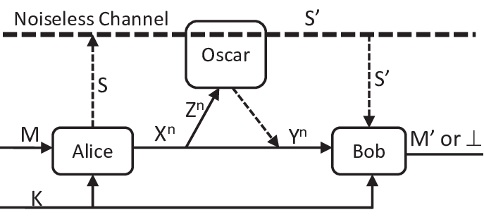
Fig. 1: The communication model.

In this paper, we consider an authentication model as follows. A legitimate transmitter Alice plans to send a message and authenticate it to receiver Bob in the presence of an adversary Oscar. It is assume that Alice and Bob share a secret key KK, and there is a DMC W1:𝒳→𝒴W_{1}:\mathcal{X}\rightarrow{\mathcal{Y}} from Alice to Bob and an one-way noiseless channel from Alice to Bob goes through Oscar. In addition, there is a DMC W2:𝒳→𝒵W_{2}:\mathcal{X}\rightarrow{\mathcal{Z}} from Alice to Oscar and a noiseless channel from Oscar to Bob (see Fig. 1 for an illustration). Practically, Internet, Telephone, or a wireless communication system with an error correcting-code can serve as this channel. We also assume that Oscar has unbounded computing resources, and can play an arbitrary man-in-the-middle attack and see a polynomial number of message authentications (details in Section III).

We study the message authentication code (MAC) in these noisy model (see Fig. 2 for an illustration): Alice encodes MM to a codeword (S,Xn)(S,X^{n}) with SS sent over the noiseless channel and XnX^{n} sent over the wiretap channel (W1,W2)(W_{1},W_{2}), which arrives at Bob as (S′,Yn)(S^{\prime},Y^{n}), where nn is the length of codeword over the noisy channel W1W_{1} and S′S^{\prime} is the received version of SS by Bob through Oscar. Upon (S′,Yn)(S^{\prime},Y^{n}), Bob decides to reject or accept the authentication by checking the consistency of (S′,Yn).(S^{\prime},Y^{n}). We regard the transmission over the wiretap channel as an expensive resource and define an efficiency measure for the MAC as authentication rate ρa​u​t​h=|M|n\rho_{auth}=\frac{|M|}{n}, where |M||M| denotes the bit length of MM.

Refer to caption
Fig. 2: The authentication model.

The goal of the paper is to propose a MAC protocol in the above model achieving a multi-messages authentication with the same secret key KK. The main efficiency criterion is a minimization of the wiretap channel usage while keeping the probability of Oscar mounting a successful attack negligible. To achieve the goal with high efficiency, we present a natural MAC scheme as follows. Alice first generates a traditional message authentication code TT of MM and uses an channel coding to encode TT to XnX^{n}. Finally, the codeword is (M,Xn)(M,X^{n}), where MM is for the noiseless channel and XnX^{n} is for channel (W1,W2)(W_{1},W_{2}). Upon (M′,Yn)(M^{\prime},Y^{n}), Bob’s verification is to check the consistency of M′M^{\prime} and YnY^{n}. The main challenge is how to design a channel coding with completeness and authentication (details of completeness and authentication in Section III). We addresses this issue by leveraging random coding techniques (details in Section IV).

In the proposed scheme, we can rewrite ρa​u​t​h=ρt​a​g⋅ρc​h​a​n\rho_{auth}=\rho_{tag}\cdot\rho_{chan}, where ρc​h​a​n=|T|n\rho_{chan}=\frac{|T|}{n} is called channel coding rate and ρt​a​g=|M||T|\rho_{tag}=\frac{|M|}{|T|} is called the rate of tag. ρt​a​g\rho_{tag} is mainly determined by purely cryptographic techniques while ρc​h​a​n\rho_{chan} is determined by channel coding techniques. The latter is our main focus. With secrecy capacity CsC_{s} of Csiszár and Körner [6] in mind, if we naturally encode TT to XnX^{n} using their code, we get ρa​u​t​h=ρt​a​g​Cs\rho_{auth}=\rho_{tag}C_{s}, which can be trivially generalized from Lai’s work [20]. This intuitively seems to be the best possible result as we have to protect TT in its full secrecy. However, we propose a new coding technique, achieving ρa​u​t​h=ρt​a​g​(H⁡(X|Z)−δ)\rho_{auth}=\rho_{tag}(H(X|Z)-\delta) for any small δ>0.\delta>0. As shown in [6], when channel W1W_{1} is less noisy than channel W2W_{2}, then Cs=H⁡(X|Z)−H⁡(X|Y)C_{s}=H(X|Z)-H(X|Y). So the ratio of authentication rate of the natural scheme to ours is arbitrarily close to 1−H⁡(X|Y)/H⁡(X|Z)<11-H(X|Y)/H(X|Z)<1. Our crucial point for this is that the secrecy capacity guarantees that Bob can recover TT while in the setting, this is unnecessary because in case of no attack, it can be computed from M′=MM^{\prime}=M and KK and in case of an attack, Bob only needs to detect the inconsistency of M′M^{\prime} and YnY^{n} and reject. How to detect the attack without fully recovering TT is the non-trivial part of our work. We achieve this through random coding techniques.

This paper is organized as follows. Section II introduces basic concepts and results that will be used in this paper. Section III introduces our authentication model. Section IV introduces our MAC. Section V proves an authentication theorem of our MAC. Section VI discusses the efficiency of our MAC. The last section is a conclusion.

II Preliminaries

In this paper, we use the following notations or conventions.

  • •

    A random variable (RV) is denoted by an upper case letter (e.g., X,YX,Y); its realization is denoted by a lower case letter (e.g., x,yx,y); its domain is denoted by a calligraphic letter (e.g., 𝒳,𝒴\mathcal{X},\mathcal{Y}); X←U𝒳X\leftarrow_{U}\mathcal{X} means that XX is chosen uniformly at random from 𝒳\mathcal{X}.

  • •

    xnx^{n} denotes a sequence x1,⋯,xnx_{1},\cdots,x_{n} of length nn. For a positive integer ss, define [s]={1,⋯,s}.[s]=\{1,\cdots,s\}.

  • •

    Probabilities P⁡(X=x)P(X=x) and P⁡(X=x|Y=y)P(X=x|Y=y) are denoted by PX​(x)P_{X}(x) and PX|Y​(x|y)P_{X|Y}(x|y). PY|Xn​(yn|xn)P^{n}_{Y|X}(y^{n}|x^{n}) is defined as ∏i=1nPY|X​(yi|xi)\prod_{i=1}^{n}P_{Y|X}(y_{i}|x_{i})

  • •

    Pxn​(⋅)P_{x^{n}}(\cdot) is a distribution over alphabet 𝒳\mathcal{X}, where for any a∈𝒳a\in\mathcal{X}, Pxn​(a)P_{x^{n}}(a) is the fraction of aa in sequence xnx^{n}. Similarly, Pxn​yn​(a,b)P_{x^{n}y^{n}}(a,b) is the fraction of (a,b)(a,b) in sequence (x1,y1),(x2,y2),⋯,(xn,yn)(x_{1},y_{1}),(x_{2},y_{2}),\cdots,(x_{n},y_{n}).

  • •

    Distance between RVs XX and X′X^{\prime} is SD​(X,X′)=∑x|PX​(x)−PX′​(x)|.\textsf{SD}(X;X^{\prime})=\sum_{x}|P_{X}(x)-P_{X^{\prime}}(x)|. Conditional distance between XX given YY and X′X^{\prime} is

    SD​(X|Y;X′)=∑y,xPY​(y)​|PX|Y​(x|y)−PX′​(x)|.\displaystyle\textsf{SD}(X|Y;X^{\prime})=\sum_{y,x}P_{Y}(y)|P_{X|Y}(x|y)-P_{X^{\prime}}(x)|.
  • •

    Entropy H(X)=−∑xPX(x)logPX(x)H(X)=-\sum_{x}P_{X}(x)\log P_{X}(x); mutual information I⁡(X,Y)=∑x,yPX​Y​(x,y)​log⁡PX​Y​(x,y)PX​(x)​PY​(y)I(X;Y)=\sum_{x,y}P_{XY}(x,y)\log\frac{P_{XY}(x,y)}{P_{X}(x)P_{Y}(y)}; conditional entropy

    H(X|Y)=−∑x,yPX​Y(x,y)logPX|Y(x|y).\displaystyle H(X|Y)=-\sum_{x,y}P_{XY}(x,y)\log P_{X|Y}(x|y).
  • •

    RVs X1,⋯,XmX_{1},\cdots,X_{m} form a Markov chain, denoted by X1→⋯→XmX_{1}\rightarrow\cdots\rightarrow X_{m}, if PXi|Xi−1⋯X1(xi|xi−1⋯x1)=PXi|Xi−1(xi|xi−1),P_{X_{i}|X_{i-1}\cdots X_{1}}(x_{i}|x_{i-1}\cdots x_{1})=P_{X_{i}|X_{i-1}}(x_{i}|x_{i-1}), for any i=2,⋯,m.i=2,\cdots,m.

The following lemma [7, Lemma 1] shows the relationship between mutual information and distance.

Lemma 1

[7] Let XX and YY be two RVs over 𝒳{\mathcal{X}} and 𝒴{\mathcal{Y}} respectively. |𝒳|≥4.|{\mathcal{X}}|\geq 4. Let Δ=SD​(X|Y;X).\Delta=\textsf{SD}(X|Y;X). Then

12​ln⁡2​Δ2≤I⁡(X,Y)≤Δ​log⁡|𝒳|Δ.\frac{1}{2\ln 2}\Delta^{2}\leq I(X;Y)\leq\Delta\log\frac{|{\mathcal{X}}|}{\Delta}. (1)

II-A ϵ\epsilon-almost strongly universal hash function

A universal hash function essentially is a family of compression functions that has an almost uniformly distributed output. It was introduced by Wegman and Carter [15] and further developed in [16, 17]. We now introduce the ϵ\epsilon-almost strongly-universal hash function.

Definition 1

A finite family of hash functions HH from alphabet ℳ\mathcal{M} to a finite alphabet 𝒯\mathcal{T} is ϵ\epsilon-almost strongly-universal (ϵ\epsilon-ASU) if the following holds

  • -

    |{h∈ℋ:h⁡(x)=t}|=|ℋ||𝒯||\{h\in\mathcal{H}:h(x)=t\}|=\frac{|\mathcal{H}|}{|\mathcal{T}|}, ∀x∈ℳ,∀t∈𝒯\forall x\in\mathcal{M},\forall t\in\mathcal{T},

  • -

    |{h∈ℋ:h(x1)=t1,h(x2)=t2}|≤ϵ​|ℋ||𝒯|,∀x1,x2∈ℳ|\{h\in\mathcal{H}:h(x_{1})=t_{1},h(x_{2})=t_{2}\}|\leq\frac{\epsilon|\mathcal{H}|}{|\mathcal{T}|},\forall x_{1},x_{2}\in\mathcal{M} (OPENx1≠x2),∀t1,t2∈𝒯.x_{1}\neq x_{2}),\forall t_{1},t_{2}\in\mathcal{T}.

We remark that domain ℳ\mathcal{M} is not necessarily finite but 𝒯\mathcal{T} and ℋ\mathcal{H} are both finite. In this paper, ℋ\mathcal{H} is indexed by elements in a set 𝒦.\mathcal{K}. We can write ℋ={hk}k∈𝒦.\mathcal{H}=\{h_{k}\}_{k\in\mathcal{K}}. So |𝒦|=|ℋ||\mathcal{K}|=|\mathcal{H}| and hkh_{k} is uniformly random in ℋ\mathcal{H} when kk is so in 𝒦.\mathcal{K}.

A construction of ϵ\epsilon-ASU hashing function with a good input/output ratio will be used in this paper. Stinson [17] showed that there exists a scheme that compresses 2s​log⁡q2^{s}\log q length to log⁡q\log q length. We state it as follows.

Lemma 2

[17] Let qq be a prime power and let s≥1s\geq 1 be an integer. Then there exists an sq\frac{s}{q}-ASU hash function from ℳ\mathcal{M} to 𝒯\mathcal{T} with key space 𝒦0\mathcal{K}_{0}, where |𝒦0|=qs|\mathcal{K}_{0}|=q^{s}, |ℳ|=q2s|\mathcal{M}|=q^{2^{s}}, |𝒯|=q|\mathcal{T}|=q.

II-B Discrete memoryless channel

A discrete memoryless channel (DMC) with input alphabet 𝒳\mathcal{X} and output alphabet 𝒴\mathcal{Y} is characterized by a stochastic matrix W={W⁡(y|x)}x∈𝒳,y∈𝒴W=\{W(y|x)\}_{x\in\mathcal{X},y\in\mathcal{Y}}, where W(⋅|x)W(\cdot|x) is the distribution of the channel output YY when the input is X=xX=x, i.e., W⁡(y|x)=PY|X​(y|x)W(y|x)=P_{Y|X}(y|x). In this case, we say XX and YY are connected by channel WW. If the input sequence is xnx^{n} and the output sequence is yny^{n}, then PYn|Xn​(yn|xn)=∏i=1nPY|X​(yi|xi)=∏i=1nW⁡(yi|xi).P_{Y^{n}|X^{n}}(y^{n}|x^{n})=\prod_{i=1}^{n}P_{Y|X}(y_{i}|x_{i})=\prod_{i=1}^{n}W(y_{i}|x_{i}). For simplicity, we denote ∏i=1nW⁡(yi|xi)\prod_{i=1}^{n}W(y_{i}|x_{i}) by W⁡(yn|xn)W(y^{n}|x^{n}).

A nn-length code 𝒞{\cal C} for a DMC W:𝒳→𝒴W:\mathcal{X}\rightarrow\mathcal{Y} with message space 𝒯\mathcal{T} is a pair of functions (f,ϕ)(f,\phi), where f:𝒯→𝒳nf:\mathcal{T}\rightarrow\mathcal{X}^{n} is the encoding function, ϕ:𝒴n→𝒯∪{⟂}\phi:\mathcal{Y}^{n}\rightarrow\mathcal{T}\cup\{\perp\} is the decoding function, and ⟂\perp denotes a detection of error. For t∈𝒯t\in\mathcal{T}, f⁡(t)∈𝒳nf(t)\in\mathcal{X}^{n} is called a codeword. When a sender wants to send message tt, he sends f⁡(t)f(t). When a receiver receives vector yn∈𝒴ny^{n}\in\mathcal{Y}^{n}, he decodes it to ϕ⁡(yn).\phi(y^{n}). If ϕ⁡(yn)≠t,\phi(y^{n})\neq t, an error occurs. The error probability of a code is defined e⁡(𝒞)=P⁡(ϕ⁡(Yn)≠T)e({\cal C})=P(\phi(Y^{n})\neq T), where YnY^{n} is the channel output with message TT that is uniformly random over 𝒯\mathcal{T}.

II-C Typical sequences

Let xnx^{n} be a sequence over 𝒳\mathcal{X}. Then the distribution Pxn​(⋅)P_{x^{n}}(\cdot) is called the type of xnx^{n} over 𝒳\mathcal{X}, where Pxn​(a)P_{x^{n}}(a) is the fraction of occurrences of aa in xnx^{n}. For a type PP over 𝒳\mathcal{X}, type set TPn\textsf{T}_{P}^{n} denotes the set of all nn-length sequences over 𝒳\mathcal{X} with type P.P.

Definition 2

Let XX be a RV over alphabet 𝒳\mathcal{X}. xn∈𝒳nx^{n}\in\mathcal{X}^{n} is ϵ\epsilon-typical if |Pxn​(a)−PX​(a)|≤ϵ|𝒳||P_{x^{n}}(a)-P_{X}(a)|\leq\frac{\epsilon}{|\mathcal{X}|} for all a∈𝒳a\in\mathcal{X}, and further it holds that Pxn​(a)=0P_{x^{n}}(a)=0 for any aa with PX​(a)=0P_{X}(a)=0. The set of ϵ\epsilon-typical sequences for XX is denoted by T[X]ϵn\textsf{T}_{[X]_{\epsilon}}^{n}.

Note that if xn∈T[X]ϵnx^{n}\in\textsf{T}_{[X]_{\epsilon}}^{n}, then the whole type set TPxnn\textsf{T}_{P_{x^{n}}}^{n} is included in T[X]ϵn.\textsf{T}_{[X]_{\epsilon}}^{n}. So T[X]ϵn\textsf{T}_{[X]_{\epsilon}}^{n} is a union of some type sets whose type is “close” to PX.P_{X}. Note the form of XX could be arbitrary. Especially, it could be a vector such as X=(Y,Z).X=(Y,Z). If xn=(yn,zn)x^{n}=(y^{n},z^{n}) is ϵ\epsilon-typical for X=(Y,Z)X=(Y,Z), we say (yn,zn)(y^{n},z^{n}) is jointly ϵ\epsilon-typical. The set of jointly ϵ\epsilon-typical sequences for YY and ZZ is denoted by T[Y​Z]ϵn.\textsf{T}_{[YZ]_{\epsilon}}^{n}.

Definition 3

Let XX and YY be RVs over alphabet 𝒳\mathcal{X} and 𝒴\mathcal{Y} respectively. yn∈𝒴ny^{n}\in\mathcal{Y}^{n} is conditionally ϵ\epsilon-typical given xn∈𝒳nx^{n}\in\mathcal{X}^{n}, if |Pxn​yn​(a,b)−Pxn​(a)​PY|X​(b|a)|≤ϵ|𝒳|⋅|𝒴||P_{x^{n}y^{n}}(a,b)-P_{x^{n}}(a)P_{Y|X}(b|a)|\leq\frac{\epsilon}{|\mathcal{X}|\cdot|\mathcal{Y}|} for all a∈𝒳a\in\mathcal{X} and b∈𝒴b\in\mathcal{Y}, and further it holds that Pxn​yn​(a,b)=0P_{x^{n}y^{n}}(a,b)=0 for any a,ba,b with PX​Y​(a,b)=0P_{XY}(a,b)=0. The set of conditionally ϵ\epsilon-typical sequences for YY, given xnx^{n}, is denoted T[Y|X]ϵn​(xn).\textsf{T}_{[Y|X]_{\epsilon}}^{n}(x^{n}). If XX and YY are connected by DMC WW, T[Y|X]ϵn​(xn)\textsf{T}_{[Y|X]_{\epsilon}}^{n}(x^{n}) is also denoted by T[W]ϵn​(xn).\textsf{T}_{[W]_{\epsilon}}^{n}(x^{n}).

We now introduce some basic properties of typical sequences, which are well-known and can be found in existing information theory books (e.g. [9, Chap 1.2]).

Lemma 3

Let X1,X2,XX_{1},X_{2},X be RVs over 𝒳\mathcal{X} and YY be a RV over 𝒴\mathcal{Y}. Then,

  • 1.

    For any type QQ of 𝒳n\mathcal{X}^{n},

    (n+1)−|𝒳|⋅2n​H​(Q)≤|TQn|≤2n​H​(Q).(n+1)^{-|\mathcal{X}|}\cdot 2^{nH(Q)}\leq|\textsf{T}_{Q}^{n}|\leq 2^{nH(Q)}.
  • 2.

    There exists constant c>0c>0 s.t. for ∀ϵ>0\forall\epsilon>0, ∀xn∈T[X]ϵn\forall x^{n}\in\textsf{T}_{[X]_{\epsilon}}^{n},

    2−n⁡[H⁡(X)+c​ϵ]≤PXn​(xn)≤2−n⁡[H⁡(X)−c​ϵ],\displaystyle 2^{-n[H(X)+c\epsilon]}\leq P_{X}^{n}(x^{n})\leq 2^{-n[H(X)-c\epsilon]},
    (1−ϵ)​2n⁡[H⁡(X)−c​ϵ]≤∗|T[X]ϵn|≤2n⁡[H⁡(X)+c​ϵ].\displaystyle(1-\epsilon)2^{n[H(X)-c\epsilon]}\stackrel{{\scriptstyle*}}{{\leq}}|\textsf{T}_{[X]_{\epsilon}}^{n}|\leq 2^{n[H(X)+c\epsilon]}.

    where inequality (∗*) holds when nn large enough.

  • 3.

    There exists constant c>0c>0 s.t. for ∀ϵ>0\forall\epsilon>0, ∀xn∈T[X]ϵn\forall x^{n}\in\textsf{T}_{[X]_{\epsilon}}^{n}, ∀yn∈T[Y|X]ϵ​(xn)\forall y^{n}\in\textsf{T}_{[Y|X]_{\epsilon}}(x^{n}),

    2−n⁡[H⁡(Y|X)+c​ϵ]≤PY|Xn​(yn|xn)≤2−n⁡[H⁡(Y|X)−c​ϵ],\displaystyle 2^{-n[H(Y|X)+c\epsilon]}\leq P_{Y|X}^{n}(y^{n}|x^{n})\leq 2^{-n[H(Y|X)-c\epsilon]},
    (1−ϵ)​2n⁡[H⁡(Y|X)−c​ϵ]≤∗|T[Y|X]ϵn​(xn)|≤2n⁡[H⁡(Y|X)+c​ϵ].\displaystyle(1-\epsilon)2^{n[H(Y|X)-c\epsilon]}\stackrel{{\scriptstyle*}}{{\leq}}|\textsf{T}_{[Y|X]_{\epsilon}}^{n}(x^{n})|\leq 2^{n[H(Y|X)+c\epsilon]}.

    where inequality (*) holds when nn large enough.

  • 4.

    There exists constants λ1\lambda_{1} and λ2>0\lambda_{2}>0 such that when nn large enough, for any xn∈T[X]ϵnx^{n}\in\textsf{T}_{[X]_{\epsilon}}^{n}

    PYn​(T[Y]ϵn)\displaystyle P_{Y}^{n}(\textsf{T}^{n}_{[Y]_{\epsilon}}) ≥\displaystyle\geq 1−2−n​λ1​ϵ2,\displaystyle 1-2^{-n\lambda_{1}\epsilon^{2}},
    PY|Xn​(T[Y|X]ϵn​(xn)|xn)\displaystyle P_{Y|X}^{n}(\textsf{T}^{n}_{[Y|X]_{\epsilon}}(x^{n})|x^{n}) ≥\displaystyle\geq 1−2−n​λ2​ϵ2.\displaystyle 1-2^{-n\lambda_{2}\epsilon^{2}}.

III MAC for a wiretap channel: the model

Syntax Model.  Assume that there is a DMC W1:𝒳→𝒴W_{1}:\mathcal{X}\rightarrow{\mathcal{Y}} from Alice to Bob. There is also an one-way noiseless channel from Alice to Bob. There is a DMC W2:𝒳→𝒵W_{2}:\mathcal{X}\rightarrow{\mathcal{Z}} from Alice to Oscar and a noiseless channel from Oscar to Bob. In this section, we will formulate the message authentication code in this channel model. It allows Alice to authenticate a message to Bob while preventing attacks from Oscar. Let ℳ{\mathcal{M}} be the message space. The system is described by an encoding function F:ℳ×𝒦→𝒮×𝒳nF:\mathcal{M}\times\mathcal{K}\rightarrow\mathcal{S}\times{\mathcal{X}^{n}} and a decoding function G:𝒦×𝒮×𝒴n→ℳ∪{⊥}G:\mathcal{K}\times\mathcal{S}\times\mathcal{Y}^{n}\rightarrow\mathcal{M}\cup\{\bot\}. The authentication syntax is as follows.

  • •

    If Alice wishes to authenticate M∈ℳM\in\mathcal{M} to Bob, she computes (S,Xn)=F⁡(M,K).(S,X^{n})=F(M,K). She then sends SS over a noiseless channel to Bob, and sends XnX^{n} over a wiretap channel (W1,W2)(W_{1},W_{2}). Through Oscar, SS will arrive at Bob as S′S^{\prime}. Let XnX^{n}, through W1W_{1}, arrive at Bob as YnY^{n} and, through W2W_{2}, arrive at Oscar as Zn.Z^{n}.

  • •

    Upon (S′,Yn)(S^{\prime},Y^{n}), Bob computes M′=G⁡(K,S′,Yn)M^{\prime}=G(K,S^{\prime},Y^{n}). If M′≠⟂M^{\prime}\neq\perp, he outputs M′M^{\prime} as the authenticated message from Alice; otherwise, he rejects.

Note if Alice does not use the noisy channel, then our model degenerates to a traditional MAC model. So naturally, we call (F,G)(F,G) a message authentication code (MAC) over channel (W1,W2)(W_{1},W_{2}) and call (S,Xn)(S,X^{n}) the codeword of MM. For our convenience, we define a decision bit D:𝒦×𝒮×𝒴n→{0,1}D:\mathcal{K}\times\mathcal{S}\times\mathcal{Y}^{n}\rightarrow\{0,1\} such that D⁡(K,S′,Yn)=0D(K,S^{\prime},Y^{n})=0 if and only if G(K,S′,Yn)=⊥G(K,S^{\prime},Y^{n})=\bot (i.e., Bob rejects).

Adversary Model.  An authentication failure could come from a completeness error or an attack from Oscar. If MAC is designed properly, the completeness error is negligible. So we focus on attacks. In our model, Oscar can arbitrarily modify SS over the noiseless channel. We assume that the channel from Oscar to Bob is noiseless and hence Oscar can launch impersonation attacks. We also allow Oscar to learn the decision bit for each authentication. Granting Oscar to learn this is not artificial. For instance, if Bob rejects the authentication, he could request Alice to re-authenticate the message. This allows Oscar to learn the decision bit b=0b=0. For another instance, if MM is one message in a serial authentication procedure (such as a stream authentication), Bob could feedback an updated message index that represents the current successfully authenticated message. This implicitly allows Oscar to learn the decision bit. We also wish to capture the concern that even if Oscar has adaptively attacked many authentication instances, he still cannot cheat Bob to accept a false authentication. The formal model is as follows.

  • I.

    Let Mi,i=1,2,⋯,M_{i},i=1,2,\cdots, be the sequence of messages authenticated by Alice. Let (Si,Xin)(S_{i},X_{i}^{n}) be the codeword of MiM_{i}. Alice sends SiS_{i} over the noiseless channel to Bob and XinX^{n}_{i} over channel (W1,W2)(W_{1},W_{2}). Oscar can revise SiS_{i} to arbitrary Si′∈𝒮.S_{i}^{\prime}\in\mathcal{S}. Let XinX_{i}^{n} arrive at Bob as YinY^{n}_{i} and at Oscar as ZinZ_{i}^{n}. Let Mi′=G⁡(K,Si′,Yin)M_{i}^{\prime}=G(K,S_{i}^{\prime},Y^{n}_{i}) and bi=D⁡(K,Si′,Yin)b_{i}=D(K,S_{i}^{\prime},Y^{n}_{i}). Besides (Si,Zin)(S_{i},Z_{i}^{n}), Oscar also learns bi.b_{i}.

    Note here we consider an adaptive Oscar. So he determines Si′S_{i}^{\prime} based on SiS_{i}, his local random source RR and the information collected previously: {(Sj,Zjn)}j=1i−1\{(S_{j},Z^{n}_{j})\}_{j=1}^{i-1} and decision bits {bj}j=1i−1\{b_{j}\}_{j=1}^{i-1} in stage I and decision bits {b^j}\{\hat{b}_{j}\} in stage II below.

  • II.

    Oscar can adaptively send S^t∈𝒮\hat{S}_{t}\in{\mathcal{S}} and Y^tn∈𝒴n\hat{Y}^{n}_{t}\in{\mathcal{Y}}^{n} to Bob noiselessly. Oscar will learn Bob’s decision bit b^t=D⁡(K,S^t,Y^n)\hat{b}_{t}=D(K,\hat{S}_{t},\hat{Y}^{n}). He succeeds if b^t=1.\hat{b}_{t}=1.

    Here (S^t,Y^tn)(\hat{S}_{t},\hat{Y}^{n}_{t}) is computed based on RR and the information collected previously: {(Sj,Zjn,bj)}\{(S_{j},Z^{n}_{j},b_{j})\} and {b^j}j=1t−1.\{\hat{b}_{j}\}_{j=1}^{t-1}.

In the model, Oscar can arbitrarily interleave Type I attacks and Type II attacks. We use succ to denote the success in a Type I or Type II attack.

Authentication Property.  After introducing the adversary model, we now define the authentication property formally. It consists of completeness and authentication. Completeness essentially states that when Oscar does not present, Bob should accept MM with high probability. Authentication states that Oscar can succeed in the above two types of attacks only with a negligible probability.

Definition 4

A message authentication code (F,G)(F,G) over channel W1:𝒳→𝒴,W2:𝒳→𝒵W_{1}:{\mathcal{X}}\rightarrow{\mathcal{Y}},W_{2}:{\mathcal{X}}\rightarrow{\mathcal{Z}} is secure if the following holds (where nn is the number of channel W1W_{1} uses).

  • 1.

    Completeness.  If Oscar does not present, then Bob rejects with exponentially (in nn) small probability.

  • 2.

    Authentication. If the number of Type II attacks is polynomially bounded (in nn), Pr⁡(s​u​c​c)\Pr({succ}) is negligible.

Remark. Restriction on the number of Type II attacks is unavoidable as Oscar can always choose a message MM and impersonate with every possible (s,yn)∈𝒮×𝒴n(s,y^{n})\in\mathcal{S}\times\mathcal{Y}^{n} to Bob. As 𝒮\mathcal{S} and 𝒴n\mathcal{Y}^{n} are finite sets, he can always succeed for some pair (s,yn).(s,y^{n}). The number of Type II attacks is chosen as be polynomially bounded as each attack will involve Bob (as a verifier) and it is impractical to require him to be in a complexity class beyond a polynomial. For the same reason, the number of Type I attacks is also polynomially bounded (implicitly), although we do not require this.

Efficiency.  We regard the communication over a wiretap channel as an expensive resource. It is desired to minimize the use of it. For convenience of analysis, we define the efficiency measure for a MAC. It is called authentication rate, defined as ρa​u​t​h=log⁡|ℳ|n\rho_{auth}=\frac{\log|\mathcal{M}|}{n}, which is the ratio of the source message length to the codeword length.

IV Our Scheme

IV-A Random coding theorem

To construct our scheme, we will prove the existence of a channel coding scheme that satisfies many strong properties. It essentially states that, there exists a set 𝒞⊆TPn\mathcal{C}\subseteq\textsf{T}_{P}^{n} such that:

(1) 𝒞\mathcal{C} can be divided into subsets {Ci​j}i,j\{C_{ij}\}_{i,j} (as shown in Fig. 3) such that each column C1​j∪⋯∪C𝕀​jC_{1j}\cup\cdots\cup C_{\mathbb{I}j} is a code for channel W1W_{1};

(2) If II is uniform random and JJ is an arbitrary RV but independent for I, then for X^n\hat{X}^{n} uniformly random over 𝒞I​J\mathcal{C}_{IJ} that is transmitted over a wiretap channel (W1,W2CLOSE(W_{1},W_{2}), the output Z^n\hat{Z}^{n} of channel W2W_{2} is almost independent of (I,J)(I,J);

(3) In item 2, if the output of W1W_{1} is Y^n\hat{Y}^{n}, then for any adversarially chosen J′J^{\prime} (that satisfies certain properties), it is unlikely that Y^n\hat{Y}^{n} can be decoded using gJ′g_{J^{\prime}} into a codeword in 𝒞I​J′.{\cal C}_{IJ^{\prime}}. The formal statement is as follows.

C11C_{11} ⋯\cdots C1​jC_{1j} ⋯\cdots C1​𝕁C_{1\mathbb{J}}
⋮\vdots ⋱\ddots ⋮\vdots ⋱\ddots ⋮\vdots
Ci​1C_{i1} ⋯\cdots Ci​jC_{ij} ⋯\cdots Ci​𝕁C_{i\mathbb{J}}
⋮\vdots ⋱\ddots ⋮\vdots ⋱\ddots ⋮\vdots
C𝕀​1C_{\mathbb{I}1} ⋯\cdots C𝕀​jC_{\mathbb{I}j} ⋯\cdots C𝕀​𝕁C_{\mathbb{I}\mathbb{J}}
Fig. 3: The codebook used in our construction.
Theorem 1

Let X,Y,ZX,Y,Z be RVs over 𝒳,𝒴,𝒵\mathcal{X,Y,Z} respectively such that PY|X=W1,PZ|X=W2P_{Y|X}=W_{1},P_{Z|X}=W_{2} for DMCs W1,W2W_{1},W_{2} and that PX=PP_{X}=P for a type PP over 𝒳\mathcal{X} with P⁡(x)>0,∀x∈𝒳P(x)>0,\forall x\in\mathcal{X}. Assume I⁡(X,Y)>I⁡(X,Z)+τI(X;Y)>I(X;Z)+\tau for some τ>0\tau>0. Then, for any integers 𝕀,𝕁{\mathbb{I}},{\mathbb{J}} with

0\displaystyle 0 ≤\displaystyle\leq 1n​log⁡𝕁<H⁡(X|Y)+τ,\displaystyle\frac{1}{n}\log{\mathbb{J}}<H(X|Y)+\tau, (2)
0\displaystyle 0 ≤\displaystyle\leq 1n​log⁡𝕀<I⁡(X,Y)−I⁡(X,Z)−τ,\displaystyle\frac{1}{n}\log{\mathbb{I}}<{I(X;Y)-I(X;Z)-\tau}, (3)

there exists disjoint subsets 𝒞i​j⊂TPn{\mathcal{C}}_{ij}\subset{\textsf{T}_{P}^{n}}, i∈[𝕀],j∈[𝕁]i\in[{\mathbb{I}}],j\in[{\mathbb{J}}] s.t. when nn large enough

  • 1.

    For each jj, 𝒞⋅j=d​e​f⋃i𝒞i​j\mathcal{C}_{\cdot j}\stackrel{{\scriptstyle def}}{{=}}\bigcup_{i}{{\mathcal{C}}_{ij}} is a code (fj,gj)(f_{j},g_{j}) for channel W1W_{1} that has an exponentially small average error probability, where fjf_{j} encodes a message mm to the mmth codeword in 𝒞⋅j\mathcal{C}_{\cdot j}.

  • 2.

    For any RV JJ over [𝕁][{\mathbb{J}}] and II over [𝕀][{\mathbb{I}}] with PI​J=PJ𝕀,P_{IJ}=\frac{P_{J}}{{\mathbb{I}}}, let Z^n\hat{Z}^{n} be the output of channel W2W_{2} with input X^n←U𝒞I​J\hat{X}^{n}\leftarrow_{U}\mathcal{C}_{IJ}. Then, I⁡(I,J,Z^n)≤2−n​β2I(I,J;\hat{Z}^{n})\leq{2^{-n\beta_{2}}}, for some β2>0\beta_{2}>0 (not depending on OPENPJ).P_{J}).

  • 3.

    For any RV JJ over [𝕁][{\mathbb{J}}] and II over [𝕀][{\mathbb{I}}] with PI​J=PJ𝕀,P_{IJ}=\frac{P_{J}}{{\mathbb{I}}}, let Y^n\hat{Y}^{n} be the output of channel W1W_{1} with input X^n←U𝒞I​J\hat{X}^{n}\leftarrow_{U}\mathcal{C}_{IJ}. Assume RV J′J^{\prime} over [𝕁][{\mathbb{J}}] with J′≠JJ^{\prime}\neq J satisfying

    • a.

      SD​(PJ′​J,PJ′​J|I)≤δ1\textsf{SD}(P_{J^{\prime}J};P_{J^{\prime}J|I})\leq\delta_{1};

    • b.

      J′→I​J→X^n→Y^nJ^{\prime}\rightarrow IJ\rightarrow\hat{X}^{n}\rightarrow\hat{Y}^{n} is a Markov chain;

    • c.

      PJ′​J​(j′,j)≤2nω𝕁⁡(𝕁−1)+d⁡(j′,j)P_{J^{\prime}J}(j^{\prime},j)\leq{\frac{2^{n^{\omega}}}{{\mathbb{J}}({\mathbb{J}}-1)}+d(j^{\prime},j)} for any j,j′j,j^{\prime} and a function d⁡(⋅,⋅)d(\cdot,\cdot) s.t. ∑j′,jd⁡(j′,j)<δ2\sum_{j^{\prime},j}d(j^{\prime},j)<\delta_{2}, where ω\omega is a constant in (0,1)(0,1).

    Then, when nn large enough,

    P⁡(gJ′​(Y^n)∈𝒞I​J′)\displaystyle P\Big(g_{J^{\prime}}(\hat{Y}^{n})\in\mathcal{C}_{IJ^{\prime}}\Big) ≤2−nω+δ1+δ2.\displaystyle\leq 2^{-{n}^{\omega}}+\delta_{1}+\delta_{2}.
Proof:

Please refer to the Appendix. ∎

IV-B Construction

Now we describe the construction of our MAC. Let W1:𝒳→𝒴W_{1}:\mathcal{X}\rightarrow{\mathcal{Y}}, W2:𝒳→𝒵W_{2}:\mathcal{X}\rightarrow{\mathcal{Z}} be the wiretap channel. Assume I⁡(X,Y)>I⁡(X,Z)+τI(X;Y)>I(X;Z)+\tau for some τ>0\tau>0 and PXP_{X} be a type PP with P⁡(x)>0P(x)>0 for any x∈𝒳x\in\mathcal{X}. Let 𝒞i​j,i=1,⋯,𝕀,j=1,⋯,𝕁{\mathcal{C}}_{ij},i=1,\cdots,{\mathbb{I}},j=1,\cdots,{\mathbb{J}} be the subsets of TPn\textsf{T}_{P}^{n} obtained in Theorem 1. Set 𝒦1={1,⋯,𝕀}.\mathcal{K}_{1}=\{1,\cdots,{\mathbb{I}}\}. Let h:ℳ×𝒦0→𝒯h:\mathcal{M}\times\mathcal{K}_{0}\rightarrow\mathcal{T} be a ϵ\epsilon-ASU hash function with key space 𝒦0\mathcal{K}_{0}, where range 𝒯⊂{1,⋯,𝕁}\mathcal{T}\subset\{1,\cdots,{\mathbb{J}}\}. Alice and Bob share a secret key K=(K0,K1)∈𝒦0×𝒦1.K=(K_{0},K_{1})\in{\mathcal{K}}_{0}\times{\mathcal{K}}_{1}. We now describe the encoding and decoding procedures.

  • 1.

    Encode. To authenticate MM, Alice computes T=hK0​(M)T=h_{K_{0}}(M), and randomly takes Xn{X}^{n} from 𝒞K1​T{\mathcal{C}}_{K_{1}T}. Then the codeword of MM is (M,Xn)(M,X^{n}), where MM is sent over the noiseless channel and Xn{X}^{n} is sent over channel (W1,W2)(W_{1},W_{2}).

  • 2.

    Decode. Upon (M′,Yn)(M^{\prime},{Y}^{n}), Bob computes T′=hK0​(M′)T^{\prime}=h_{K_{0}}(M^{\prime}). If gT′​(Yn)∈𝒞K1​T′g_{T^{\prime}}(Y^{n})\in\mathcal{C}_{K_{1}T^{\prime}}, he accepts M′M^{\prime}; otherwise, he rejects, where gjg_{j} is the decoder of code 𝒞⋅j\mathcal{C}_{\cdot j}.

    Note: In the code 𝒞⋅j\mathcal{C}_{\cdot j} at Theorem 1, encoder fjf_{j} encodes message ℓ\ell to the ℓ\ellth codeword in 𝒞⋅j\mathcal{C}_{\cdot j}, gj​(Yn)g_{j}(Y^{n}) must decode to ⟂\perp or a codeword’s index in 𝒞⋅T′\mathcal{C}_{\cdot T^{\prime}}. As an index is 1-1 correspondent to its codeword, we assume gj​(Yn)g_{j}(Y^{n}) decodes to ⟂\perp or the codeword itself.

V Security Analysis

In this section, we prove the authentication property of our MAC. We begin with two lemmas. The first lemma shows that Oscar obtains no significant amount of information about secret key (K0,K1)(K_{0},K_{1}), after eavesdropping JJ times of authentications that gives Oscar information M1Z1n⋯MJZJnM_{1}Z_{1}^{n}\cdots M_{J}Z_{J}^{n}. The idea is as follows. Let Tj=hK0​(MJ)T_{j}=h_{K_{0}}(M_{J}). From Theorem 1(2), it is easy to see that I⁡(K1​Tj;Zjn|Mj=mj)≈0.I(K_{1}T_{j};Z_{j}^{n}|M_{j}=m_{j})\approx 0. Note that given Mj=mjM_{j}=m_{j}, K0​K1→K1​Tj→ZjnK_{0}K_{1}\rightarrow K_{1}T_{j}\rightarrow Z_{j}^{n} forms a Markov chain as ZjnZ_{j}^{n} is decided by K1​TjK_{1}T_{j} and some randomness independent of K0​K1K_{0}K_{1}. So by data processing inequality, I⁡(K0​K1;Zjn|Mj=mj)≤I⁡(K1​Tj;Zjn|Mj=mj)≈0.I(K_{0}K_{1};Z_{j}^{n}|M_{j}=m_{j})\leq I(K_{1}T_{j};Z_{j}^{n}|M_{j}=m_{j})\approx 0. As K0​K1K_{0}K_{1} is independent of MJM^{J}, I(K0K1;MJZ1n⋯ZJn)=I(K0K1;Z1n⋯ZJn|MJ).I(K_{0}K_{1};M^{J}Z^{n}_{1}\cdots Z_{J}^{n})=I(K_{0}K_{1};Z_{1}^{n}\cdots Z_{J}^{n}|M^{J}). Finally, by standard information theory techniques, we can show that this is bounded by ∑j=1JI⁡(K0​K1;Zjn|MJ=mJ)\sum_{j=1}^{J}I(K_{0}K_{1};Z_{j}^{n}|M^{J}=m^{J}), which is now known small. The lemma follows by averaging on MJ.M^{J}. We implement the strategy formally in the following lemma.

Lemma 4

Let (K0,K1)(K_{0},K_{1}) be uniformly distributed over 𝒦0×𝒦1\mathcal{K}_{0}\times{\mathcal{K}_{1}} and M1,⋯,MJM_{1},\cdots,M_{J} be JJ arbitrary messages in ℳ{\cal M} authenticated by Alice. For j=1,⋯,J,j=1,\cdots,J, let ZjnZ^{n}_{j} be the output of W2W_{2} when Alice sends XjnX^{n}_{j} (w.r.t. MjM_{j}). Then, there exists β2>0\beta_{2}>0 such that when nn large enough,

I(K0K1;M1Z1n⋯MJZJn)≤J⋅2−n​β2.I(K_{0}K_{1};M_{1}Z^{n}_{1}\cdots M_{J}Z^{n}_{J})\leq{J\cdot 2^{-n\beta_{2}}}. (4)
Proof:

For j=1,⋯,J,j=1,\cdots,J, let Tj=hK0​(Mj).T_{j}=h_{K_{0}}(M_{j}). Define MJ=M1⋯MJM^{J}=M_{1}\cdots M_{J} and mJ=m1⋯mJm^{J}=m_{1}\cdots m_{J} for mj∈ℳ.m_{j}\in{\cal M}. Then, PK1​Tj|MJ​(k1,tj|mJ)=PK1​(k1)​PTj|MJ​(tj|mJ)P_{K_{1}T_{j}|M^{J}}(k_{1},t_{j}|m^{J})=P_{K_{1}}(k_{1})P_{T_{j}|M^{J}}(t_{j}|m^{J}) as K1K_{1} is independent of MJM^{J} and K0.K_{0}. Reformatting this, we have PK1​Tj|MJ=mJ​(k1,tj)=PK1​(k1)​PTj|MJ=mJ​(tj)=PTj|MJ=mJ​(tj)/|𝒦1|.P_{K_{1}T_{j}|M^{J}=m^{J}}(k_{1},t_{j})=P_{K_{1}}(k_{1})P_{T_{j}|M^{J}=m^{J}}(t_{j})=P_{T_{j}|M^{J}=m^{J}}(t_{j})/|\mathcal{K}_{1}|. That is, if we rewrite the joint distribution of K1,TjK_{1},T_{j} when MJ=mJM^{J}=m^{J}, as PK1​TjmJP^{m^{J}}_{K_{1}T_{j}}, then PK1​TjmJ=PTjmJ/|𝒦1|.P^{m^{J}}_{K_{1}T_{j}}=P_{T_{j}}^{m^{J}}/|\mathcal{K}_{1}|. Hence, by Theorem 1 (property 2), when nn sufficiently large, we have I⁡(K1,Tj;Zn|MJ=mJ)≤2−n​β2I(K_{1},T_{j};Z^{n}|M^{J}=m^{J})\leq{2^{-n\beta_{2}}} for some β2>0\beta_{2}>0, where β2\beta_{2} does not depend on mJ.m^{J}.

Given MJ=mJ,M^{J}=m^{J}, we have that (K0,K1)→(Tj,K1)→Zjn(K_{0},K_{1})\rightarrow(T_{j},K_{1})\rightarrow Z_{j}^{n} forms a Markov chain. Hence, by data processing inequality, we have I⁡(K0​K1;Zjn|MJ=mJ)≤I⁡(K1​Tj;Zjn|MJ=mJ)≤2−n​β2.I(K_{0}K_{1};Z^{n}_{j}|M^{J}=m^{J})\leq I(K_{1}T_{j};Z^{n}_{j}|M^{J}=m^{J})\leq 2^{-n\beta_{2}}. Thus, averaging over mJm^{J}, we have I⁡(K0​K1;Zjn|MJ)≤I⁡(K1​Tj;Zjn|MJ)≤2−n​β2.I(K_{0}K_{1};Z^{n}_{j}|M^{J})\leq I(K_{1}T_{j};Z_{j}^{n}|M^{J})\leq 2^{-n\beta_{2}}.

Further, for any j∈{1,⋯,J}j\in\{1,\cdots,J\} and when MJ=mJM^{J}=m^{J},

Zn1⋯Znj−1→K0K1→ZnjZ^{n}_{1}\cdots Z^{n}_{j-1}\rightarrow K_{0}K_{1}\rightarrow Z^{n}_{j}

forms a Markov chain as XjnX^{n}_{j} is determined by (K0​K1K_{0}K_{1}, mJm^{J}) and the randomness of sampling XjnX^{n}_{j} from 𝒞K1​Tj\mathcal{C}_{K_{1}T_{j}}, and ZjnZ_{j}^{n} is determined by XjnX_{j}^{n} and the noise in channel W2W_{2}. Hence,

I(K0K1;Zjn|Z1n⋯Zj−1n,MJ=mJ)\displaystyle I(K_{0}K_{1};Z^{n}_{j}|Z^{n}_{1}\cdots Z^{n}_{j-1},M^{J}=m^{J})
≤I⁡(K0​K1;Zjn|MJ=mJ).\displaystyle\leq{I(K_{0}K_{1};Z_{j}^{n}|M^{J}=m^{J})}.

Averaging over mJm^{J}, we have

I(K0K1;Zjn|Z1n⋯Zj−1nMJ)≤I(K0K1;Zjn|MJ).\displaystyle I(K_{0}K_{1};Z^{n}_{j}|Z^{n}_{1}\cdots Z^{n}_{j-1}M^{J})\leq{I(K_{0}K_{1};Z_{j}^{n}|M^{J})}. (5)

Hence, by chain rule of mutual information,

I(K0K1;Z1n⋯ZJnMJ)\displaystyle I(K_{0}K_{1};Z^{n}_{1}\cdots Z^{n}_{J}M^{J})
=\displaystyle= I(K0K1;MJ)+I(K0K1;Z1n⋯ZJn|MJ)\displaystyle I(K_{0}K_{1};M^{J})+I(K_{0}K_{1};Z^{n}_{1}\cdots Z^{n}_{J}|M^{J})
=\displaystyle= I(K0K1;Z1n⋯ZJn|MJ),(K0​K1 is indep of MJ)\displaystyle I(K_{0}K_{1};Z^{n}_{1}\cdots Z^{n}_{J}|M^{J}),\quad(\mbox{$K_{0}K_{1}$ is indep of $M^{J}$})
≤\displaystyle\leq ∑jI⁡(K0​K1;Zjn|MJ)≤J​2−n​β2.\displaystyle\sum_{j}{I(K_{0}K_{1};Z_{j}^{n}|M^{J})}\leq J2^{-n\beta_{2}}.

This concludes our proof. ∎

The second lemma will be used to show that the conditional distribution of secret key on the decision bit is almost uniform.

Lemma 5

Let KK and VV be RVs over 𝒦\mathcal{K} and 𝒱\mathcal{V} respectively. Then for any v∈𝒱v\in\mathcal{V} and any 𝒦v⊆𝒦\mathcal{K}_{v}\subseteq\mathcal{K},

|PK|V=v​(𝒦v)−PK​(𝒦v)|≤12​SD​(PK|V=v,PK).{|}P_{K|V=v}{(}\mathcal{K}_{v}{)}-P_{K}{(}\mathcal{K}_{v}{)}{|}\leq\frac{1}{2}\textsf{SD}(P_{K|V=v};P_{K}). (6)
Proof:

As SD​(PX1,PX2)=2​maxA⊆𝒳​{PX1​(A)−PX2​(A)}\textsf{SD}(P_{X_{1}};P_{X_{2}})=2\max_{A\subseteq\mathcal{X}}\{P_{X_{1}}(A)-P_{X_{2}}(A)\} for any RVs X1,X2X_{1},X_{2} over 𝒳\mathcal{X}, PK|V=v​(𝒦v)−PK​(𝒦v)≤12​SD​(PK|V=v,PK).P_{K|V=v}(\mathcal{K}_{v})-P_{K}(\mathcal{K}_{v})\leq\frac{1}{2}\textsf{SD}(P_{K|V=v};P_{K}). Similarly, −PK|V=v​(𝒦v)+PK​(𝒦v)≤12​SD​(PK|V=v,PK).-P_{K|V=v}(\mathcal{K}_{v})+P_{K}(\mathcal{K}_{v})\leq\frac{1}{2}\textsf{SD}(P_{K|V=v};P_{K}). Hence, the lemma follows. ∎

The following lemmas will useful in our security proof later. Lemma 6 means that T′​TT^{\prime}T and KK are almost independent. It will be used to assign a value for δ1\delta_{1} in Theorem 1 (3-a).

Lemma 6

Let {hk0}k0∈𝒦0\{h_{k_{0}}\}_{k_{0}\in\mathcal{K}_{0}} be any family of functions from ℳ\mathcal{M} to 𝒯\mathcal{T}. Let K0,K1,U,M′,MK_{0},K_{1},U,M^{\prime},M be RVs over 𝒦0,𝒦1,𝒰,ℳ\mathcal{K}_{0},\mathcal{K}_{1},\mathcal{U},\mathcal{M} and ℳ\mathcal{M} respectively with M′,MM^{\prime},M being deterministic in UU. Assume K1K_{1} is independent of (K0,M)(K_{0},M). Let T′=hK0​(M′)T^{\prime}=h_{K_{0}}(M^{\prime}) and T=hK0​(M)T=h_{K_{0}}(M). Then, for Δ=SD​(K0​K1|U;K0​K1),\Delta=\textsf{SD}(K_{0}K_{1}|U;K_{0}K_{1}),

SD​(PT′​T|K1,PT′​T)≤2​Δ​ln⁡|𝒦0|​|𝒦1|Δ.\displaystyle\textsf{SD}(P_{T^{\prime}T|K_{1}};P_{T^{\prime}T})\leq\sqrt{2\Delta\ln\frac{|\mathcal{K}_{0}||\mathcal{K}_{1}|}{\Delta}}. (7)
Proof:

We have

I⁡(T′;K1|T)≤I⁡(U​K0;K1|T)\displaystyle I(T^{\prime};K_{1}|T)\leq{I(UK_{0};K_{1}|T)}
=\displaystyle= I⁡(U;K1|T​K0), (as I⁡(K0;K1|T)=0)\displaystyle I(U;K_{1}|TK_{0}),\quad\mbox{ (as $I(K_{0};K_{1}|T)=0$)}
=\displaystyle= H⁡(K1|T​K0)−H⁡(K1|U​T​K0)\displaystyle H(K_{1}|TK_{0})-H(K_{1}|UTK_{0})
=\displaystyle= H⁡(K1)−H⁡(K1|U​K0),\displaystyle H(K_{1})-H(K_{1}|UK_{0}),
(K1K_{1} is ind. of T​K0TK_{0}; K0​UK_{0}U determines TT)
=\displaystyle= I⁡(K1,U​K0)\displaystyle I(K_{1};UK_{0})
=\displaystyle= I⁡(K1;U|K0),(K0 and K1 are ind.)\displaystyle I(K_{1};U|K_{0}),\quad\mbox{($K_{0}$ and $K_{1}$ are ind.)}
≤\displaystyle\leq I⁡(K0​K1,U).\displaystyle I(K_{0}K_{1};U).

On the other hand, by Lemma 1,

I⁡(T′;K1|T=t)\displaystyle I(T^{\prime};K_{1}|T=t)
≥\displaystyle\geq (∑k1PK1|T=t​(k1)​SD​(PT′|T=t,PT′|K1​T=k1​t))22​ln⁡2.\displaystyle\frac{\left(\sum_{k_{1}}P_{K_{1}|T=t}(k_{1})\textsf{SD}(P_{T^{\prime}|T=t};P_{T^{\prime}|K_{1}T=k_{1}t})\right)^{2}}{2\ln 2}.

By the convexity of f⁡(x)=x2,f(x)=x^{2}, we have

I⁡(T′;K1|T)=∑tPT​(t)​I​(T′;K1|T=t)\displaystyle I(T^{\prime};K_{1}|T)=\sum_{t}P_{T}(t)I(T^{\prime};K_{1}|T=t)
≥(∑k1,tPK1​T​(k1,t)​SD​(PT′|T=t,PT′|K1​T=k1​t))22​ln⁡2.\displaystyle\geq\frac{\left(\sum_{k_{1},t}P_{K_{1}T}(k_{1},t)\textsf{SD}(P_{T^{\prime}|T=t};P_{T^{\prime}|K_{1}T=k_{1}t})\right)^{2}}{2\ln 2}.

So

∑k1,tPK1​T​(k1,t)​SD​(PT′|T=t,PT′|K1​T=k1​t)\displaystyle\sum_{k_{1},t}P_{K_{1}T}(k_{1},t)\textsf{SD}(P_{T^{\prime}|T=t};P_{T^{\prime}|K_{1}T=k_{1}t})
≤\displaystyle\leq 2​I​(K0​K1,U)​ln⁡2.\displaystyle\sqrt{2I(K_{0}K_{1};U)\ln 2}.

Independence between K1K_{1} and TT together with Lemma 1 gives the result (after reformatting the left side). ∎

The following lemma will be used to assign a value for δ2\delta_{2} in Theorem 1 (3-c) and to show that the third condition in Theorem 1 (3) can be satisfied.

Lemma 7

Let {hk0}k0∈𝒦0\{h_{k_{0}}\}_{k_{0}\in\mathcal{K}_{0}} be a family of ϵ\epsilon-ASU hash functions from ℳ\mathcal{M} to 𝒯\mathcal{T}. Let U,M′,MU,M^{\prime},M be RVs over 𝒰,ℳ\mathcal{U},\mathcal{M} and ℳ\mathcal{M} respectively s.t. M′,MM^{\prime},M are deterministic in UU. Let K0K_{0} be uniformly random over 𝒦0\mathcal{K}_{0}, T′=hK0​(M′)T^{\prime}=h_{K_{0}}(M^{\prime}) and T=hK0​(M)T=h_{K_{0}}(M). If P⁡(M′=M)=0P({M^{\prime}}=M)=0, then there exists function d⁡(t′,t)d(t^{\prime},t) s.t. ∑t′,td⁡(t′,t)≤SD​(K0|U;K0)\sum_{t^{\prime},t}d(t^{\prime},t)\leq\textsf{SD}(K_{0}|U;K_{0}) and

PT′​T​(t′,t)≤d⁡(t′,t)+ϵ|𝒯|.\displaystyle P_{T^{\prime}T}(t^{\prime},t)\leq d(t^{\prime},t)+\frac{\epsilon}{|\mathcal{T}|}.
Proof:

Let 𝒦0​(u,t′,t)\mathcal{K}_{0}(u,t^{\prime},t) be the set of k0k_{0} so that hk0​(m′)=t′h_{k_{0}}(m^{\prime})=t^{\prime} and hk0​(m)=th_{k_{0}}(m)=t, where m′,mm^{\prime},m are the values of M′M^{\prime} and MM determined by U=u.U=u. Let d⁡(t′,t)=∑u|PK0​U​(𝒦0​(u,t′,t),u)−PK0​(𝒦0​(u,t′,t))​PU​(u)|.d(t^{\prime},t)=\sum_{u}|P_{K_{0}U}(\mathcal{K}_{0}(u,t^{\prime},t),u)-P_{K_{0}}(\mathcal{K}_{0}(u,t^{\prime},t))P_{U}(u)|. Then,

PT′​T​(t′,t)\displaystyle P_{T^{\prime}T}(t^{\prime},t) =\displaystyle= ∑uPK0​U​(𝒦0​(u,t′,t),u)\displaystyle\sum_{u}P_{K_{0}U}(\mathcal{K}_{0}(u,t^{\prime},t),u)
≤\displaystyle\leq d⁡(t′,t)+∑uPK0​(𝒦0​(u,t′,t)​PU​(u)CLOSE\displaystyle d(t^{\prime},t)+\sum_{u}P_{K_{0}}(\mathcal{K}_{0}(u,t^{\prime},t)P_{U}(u)
≤\displaystyle\leq d⁡(t′,t)+ϵ|𝒯|,as |𝒦0​(u,t′,t)|≤ϵ​|𝒦0||𝒯|\displaystyle d(t^{\prime},t)+\frac{\epsilon}{|\mathcal{T}|},\quad\mbox{as $|\mathcal{K}_{0}(u,t^{\prime},t)|\leq\frac{\epsilon|\mathcal{K}_{0}|}{|\mathcal{T}|}$}

For any uu, {𝒦0​(u,t,t′)}t,t′\{\mathcal{K}_{0}({u},t,t^{\prime})\}_{t,t^{\prime}} are disjoint. Hence,

SD​(K0|U;K0)\displaystyle\textsf{SD}(K_{0}|U;K_{0})
=\displaystyle= ∑k0,u|PK0​U​(k0,u)−PK0​(k0)​PU​(u)|\displaystyle\sum_{k_{0},u}|P_{K_{0}U}(k_{0},u)-P_{K_{0}}(k_{0})P_{U}(u)|
≥\displaystyle\geq ∑t,t′,u|PK0​U​(𝒦0​(u,t′,t),u)−PK0​(𝒦0​(u,t′,t))​PU​(u)|\displaystyle\sum_{t,t^{\prime},u}|P_{K_{0}U}(\mathcal{K}_{0}(u,t^{\prime},t),u)-P_{K_{0}}(\mathcal{K}_{0}(u,t^{\prime},t))P_{U}(u)|
=\displaystyle= ∑t,t′d⁡(t′,t).\displaystyle\sum_{t,t^{\prime}}d(t^{\prime},t).

This completes the proof. ∎

V-A Authentication Theorem

Now we prove our authentication theorem. We need to show that sender Alice can authenticate polynomial number of messages using (K0,K1)(K_{0},K_{1}), where the attacker Oscar can adaptively interleave two types of attacks. In Type I attack, when Alice sends out (M,Xn)(M,X^{n}), Oscar can revise MM to M′(≠M)M^{\prime}(\neq M); in Type II attack, Oscar can send any pair (M^,Y^n)(\hat{M},\hat{Y}^{n}) to Bob noiselessly. Oscar succeeds, if gT′​(Yn)∈𝒞K1​T′g_{T^{\prime}}(Y^{n})\in{\cal C}_{K_{1}T^{\prime}} in a Type I attack (where T′=hK0​(M′)T^{\prime}=h_{K_{0}}(M^{\prime})), or gT^​(Y^n)∈𝒞K1​T^g_{\hat{T}}(\hat{Y}^{n})\in{\cal C}_{K_{1}\hat{T}} in a Type II attack (where T^=hK0​(M^)\hat{T}=h_{K_{0}}(\hat{M})). Our proof idea is as follows. We use bit bℓ=1b_{\ell}=1 to denote the success of Oscar in the ℓ\ellth attack (either Type I or Type II). In a type I attack, there are two cases: (1) hK0​(M′)=hK0​(M)h_{K_{0}}(M^{\prime})=h_{K_{0}}(M) (i.e., T=T′T=T^{\prime}), in which case Oscar succeeds with high probability by the completeness of the coding scheme (f,g);(f,g); (2) gT′​(Yn)∈𝒞K1​T′g_{T^{\prime}}(Y^{n})\in{\cal C}_{K_{1}T^{\prime}} but T≠T′T\neq T^{\prime}. For case (1), if M′M^{\prime} is independent of K0K_{0}, then the success of Oscar occurs with probability ϵ\epsilon by the property of hh. Conceivably, if M′M^{\prime} is almost independent of K0K_{0} (i.e., SD​(K0|M′;K0)\textsf{SD}(K_{0}|M^{\prime};K_{0}) is small), Oscar still succeeds with a small probability. Notice that M′M^{\prime} is determined by the view UℓU_{\ell} of Oscar. Hence, it suffices to show that SD​(K0|Uℓ;K0)\textsf{SD}(K_{0}|U_{\ell};K_{0}) is small. For case (2), we can use Theorem 1 (3) to show that the success probability is small. For type II attack, if (M^,Y^)(\hat{M},\hat{Y}) (determined by OPENUℓ)U_{\ell}) is independent of K1K_{1}, then gT^​(Y^n)∈𝒞K1​T^g_{\hat{T}}(\hat{Y}^{n})\in{\cal C}_{K_{1}\hat{T}} holds with probability 1|𝕂1|\frac{1}{|\mathbb{K}_{1}|}. Conceivably, if SD​(K1|Uℓ;K1)\textsf{SD}(K_{1}|U_{\ell};K_{1}) is small, then this should hold with a small success probability change. As SD​(Kc|Uℓ;Kc)≤SD​(K0​K1|Uℓ;K0​K1)\textsf{SD}(K_{c}|U_{\ell};K_{c})\leq\textsf{SD}(K_{0}K_{1}|U_{\ell};K_{0}K_{1}) for c=0,1,c=0,1, we only need to prove that SD​(K0​K1|Uℓ;K0​K1)\textsf{SD}(K_{0}K_{1}|U_{\ell};K_{0}K_{1}) is small, which can be done by properly combining Lemmas 4-7.

Theorem 2

Let I⁡(X,Y)≥I⁡(X,Z)+τI(X;Y)\geq I(X;Z)+\tau, where Y,ZY,Z are the outputs of W1,W2W_{1},W_{2} with input XX and PXP_{X} is a type PP with P⁡(x)>0,∀x∈𝒳P(x)>0,\forall x\in\mathcal{X}. Assume h:ℳ×𝒦0→𝒯h:{\mathcal{M}}\times{\mathcal{K}}_{0}\rightarrow{\mathcal{T}} is an ϵ\epsilon-ASU hash function with ϵ=min⁡{2−Ω⁡(log⁡n),2nω|𝒯|}\epsilon=\min\{2^{-\Omega(\log n)},\frac{2^{n^{\omega}}}{|\mathcal{T}|}\} for some ω∈(0,1)\omega\in(0,1) and |𝒦1|=2Ω⁡(log⁡n)|\mathcal{K}_{1}|=2^{\Omega(\log n)}, where g⁡(n)=Ω⁡(log⁡n)g(n)=\Omega(\log n) if limn→∞g⁡(n)log⁡n=∞\lim_{n\rightarrow\infty}\frac{g(n)}{\log n}=\infty. Then, our MAC is secure.

Proof:

From Theorem 1 (1), the completeness of the MAC holds. Now we concentrate on the authentication property.

Let Mν=M1⋯MνM^{\nu}=M_{1}\cdots M_{\nu} be the sequence of messages authenticated from Alice to Bob and Xin,ZinX_{i}^{n},Z_{i}^{n} be the input and output w.r.t. MiM_{i} over channel W2W_{2}. Note MνM^{\nu} is chosen by Alice according to distribution PMνP_{M^{\nu}} (especially independent of Oscar’s random tape RR); XinX_{i}^{n} is determined by (K0​K1,Mi)(K_{0}K_{1},M_{i}) together with the randomness of sampling XinX_{i}^{n} from 𝒞K1​T\mathcal{C}_{K_{1}T}; ZinZ_{i}^{n} is determined by XinX_{i}^{n} together with the noise in channel W2W_{2}. It follows that (Mν,K0K1,X1nZ1n⋯XνnZνn)(M^{\nu},K_{0}K_{1},X^{n}_{1}Z_{1}^{n}\cdots X_{\nu}^{n}Z_{\nu}^{n}) is independent of RR and hence has the same distribution as when Oscar does not present. Hence, by Lemma 4, I(K0K1;MjZ1n⋯Zjn)≤j2−n​β2,I(K_{0}K_{1};M^{j}Z_{1}^{n}\cdots Z_{j}^{n})\leq j2^{-n\beta_{2}}, for a constant β2>0\beta_{2}>0 and any j≤νj\leq\nu.

As (Mj,K0K1,X1nZ1n⋯XjnZjn)(M^{j},K_{0}K_{1},X^{n}_{1}Z_{1}^{n}\cdots X_{j}^{n}Z_{j}^{n}) is independent of RR, I(K0K1;RMjZ1n⋯Zjn)≤j2−n​β2I(K_{0}K_{1};RM^{j}Z_{1}^{n}\cdots Z_{j}^{n})\leq j2^{-n\beta_{2}}. Let K=d​e​fK0​K1K\stackrel{{\scriptstyle def}}{{=}}K_{0}K_{1} and Vj=d​e​fRMjZ1n⋯ZjnV_{j}\stackrel{{\scriptstyle def}}{{=}}RM^{j}Z_{1}^{n}\cdots Z_{j}^{n}. By Lemma 1,

SD(K|Vj;K)≤2​j​ln⁡2⋅2−nβ2/2.\displaystyle\textsf{SD}(K|V_{j};K)\leq\sqrt{2j\ln 2}\cdot 2^{-n\beta_{2}/2}. (8)

According to the adversary model, Oscar can adaptively interleave the following attacks.

  • I.

    When Alice sends out (Mj,Xjn)(M_{j},X_{j}^{n}), Oscar can revise MjM_{j} to Mj′(≠Mj)M_{j}^{\prime}(\neq M_{j}). He succeeds if Bob accepts (Mj′,Yjn)(M_{j}^{\prime},Y_{j}^{n}).

  • II.

    At any time, Oscar can send a pair (M^,Y^n)(\hat{M},\hat{Y}^{n}) to Bob noiselessly. He succeeds if Bob accepts this pair.

We use bit bℓb_{\ell} to denote the result of the ℓ\ellth attack (either type I or type II above) and set bℓ=1b_{\ell}=1 if and only if he succeeds.

Assume the authentication of Mjℓ−1M^{j_{\ell}-1} by Alice has been completed before Oscar launches the ℓ\ellth attack. Then, the view of Oscar right before the ℓ\ellth attack is Uℓ:=(Vjℓ−1,b1,⋯,bℓ−1),U_{\ell}:=(V_{j_{\ell}-1},b_{1},\cdots,b_{\ell-1}), where a party’s view is defined as his random tape RR and the data received externally.

If the ℓ\ellth attack is Type I, then bℓ=1b_{\ell}=1 iff gTjℓ′​(Yjℓn)∈𝒞K1​Tjℓ′g_{T_{j_{\ell}}^{\prime}}(Y^{n}_{j_{\ell}})\in\mathcal{C}_{K_{1}T_{j_{\ell}}^{\prime}} for Tjℓ′=hK0​(Mjℓ′)T^{\prime}_{j_{\ell}}=h_{K_{0}}(M_{j_{\ell}}^{\prime}). If we define event Tjℓ′=Tjℓ(:=hK0​(Mjℓ))T^{\prime}_{j_{\ell}}=T_{j_{\ell}}(:=h_{K_{0}}(M_{j_{\ell}})) by colℓ, and event gTjℓ′​(Yjℓn)∈𝒞K1​Tjℓ′g_{T_{j_{\ell}}^{\prime}}(Y^{n}_{j_{\ell}})\in\mathcal{C}_{K_{1}T_{j_{\ell}}^{\prime}} with Tjℓ≠Tjℓ′T_{j_{\ell}}\neq T_{j_{\ell}}^{\prime}, by misℓ\textsf{mis}_{\ell}, then P⁡(bℓ=1)=P⁡(colℓ)+P⁡(misℓ).P(b_{\ell}=1)=P(\textsf{col}_{\ell})+P(\textsf{mis}_{\ell}).

If the ℓ\ellth attack is Type II, then bℓ=1b_{\ell}=1 iff gT^ℓ​(Y^ℓn)∈𝒞K1​T^ℓg_{\hat{T}_{\ell}}(\hat{Y}^{n}_{\ell})\in\mathcal{C}_{K_{1}\hat{T}_{\ell}} for T^ℓ=hK0​(M^ℓ),\hat{T}_{\ell}=h_{K_{0}}(\hat{M}_{\ell}), where (M^ℓ,Y^ℓn)(\hat{M}_{\ell},\hat{Y}^{n}_{\ell}) is Oscar’s output in this attack.

If LL is the upper bound on the number of attacks by Oscar, then his success probability is Pr(∨ℓ=1Lbℓ=1).\Pr\left(\vee_{\ell=1}^{L}b_{\ell}=1\right).

As every successful attacker must experience the first successful attack, we restrict to an attacker who will stop after the first successful attack. So bℓ=1b_{\ell}=1 implies b1=⋯=bℓ−1=0.b_{1}=\cdots=b_{\ell-1}=0.

Denote the original authentication game by Γ\Gamma. Now we modify Γ\Gamma to Γ′\Gamma^{\prime} such that in Type I attack, bℓ=d​e​fcolℓb_{\ell}\stackrel{{\scriptstyle def}}{{=}}\textsf{col}_{\ell} (instead of bℓ=d​e​fcolℓ∨misℓb_{\ell}\stackrel{{\scriptstyle def}}{{=}}\textsf{col}_{\ell}\vee\textsf{mis}_{\ell}).

Consider an adversary Oscar′ for Γ′\Gamma^{\prime} who simply follows the code of Oscar by setting each (unknown) misℓ as 0 (even if it is 1). The view of Oscar′ in Γ′\Gamma^{\prime} differs from that of Oscar in Γ\Gamma only if misℓ=1\textsf{mis}_{\ell}=1 in Γ′\Gamma^{\prime} for some ℓ\ell. Thus,

P⁡(s​u​c​c​(Γ))≤P⁡(s​u​c​c​(Γ′))+∑ℓP⁡(misℓ​(Γ′)).P(succ(\Gamma))\leq P(succ(\Gamma^{\prime}))+\sum_{\ell}P(\textsf{mis}_{\ell}(\Gamma^{\prime})). (9)

As P⁡(s​u​c​c​(Γ′))≤∑ℓ=1LP⁡(bℓ​(Γ′)=1)P(succ(\Gamma^{\prime}))\leq\sum_{\ell=1}^{L}P(b_{\ell}(\Gamma^{\prime})=1), we only need to bound P⁡(bℓ​(Γ′)=1)P(b_{\ell}(\Gamma^{\prime})=1) and P⁡(misℓ​(Γ′))P(\textsf{mis}_{\ell}(\Gamma^{\prime})).

Bounding P⁡(misℓ​(Γ′))P(\textsf{mis}_{\ell}(\Gamma^{\prime})).  We have the following lemma.

Lemma 8

P⁡(misℓ​(Γ′))≤2−ς​nω+2​Δ​ln⁡|𝒦0|​|𝒦1|Δ+ΔP(\textsf{mis}_{\ell}(\Gamma^{\prime}))\leq 2^{-\varsigma{n}^{\omega}}+\sqrt{2\Delta\ln\frac{|\mathcal{K}_{0}||\mathcal{K}_{1}|}{\Delta}}+\Delta for a constant ς>0\varsigma>0, where Δ=SD​(K|Uℓ;K)\Delta=\textsf{SD}(K|U_{\ell};K).

Proof. We first show that Uℓ​Mjℓ→K1​Tjℓ→Xjℓn→YjℓnU_{\ell}M_{j_{\ell}}\rightarrow K_{1}T_{j_{\ell}}\rightarrow X^{n}_{j_{\ell}}\rightarrow Y^{n}_{j_{\ell}} forms a Markov chain. This follows from two facts:

(a)  Given XjℓnX^{n}_{j_{\ell}}, YjℓnY^{n}_{j_{\ell}} is completely determined by the noise in channel W1W_{1} while this noise occurs after fixing (Xjℓn,K1​Tjℓ​Uℓ​Mjℓ)(X^{n}_{j_{\ell}},K_{1}T_{j_{\ell}}U_{\ell}M_{j_{\ell}}) and hence is independent of the latter;

(b)  Given K1​TjℓK_{1}T_{j_{\ell}}, XjℓnX_{j_{\ell}}^{n} is determined by the randomness for sampling it from 𝒞K1​Tjℓ\mathcal{C}_{K_{1}T_{j_{\ell}}}, which is independent of Uℓ​MjℓU_{\ell}M_{j_{\ell}}.

By Theorem 1(3) with δ1\delta_{1} from Lemma 7 and δ2\delta_{2} from Lemma 6, together with the fact SD​(K0|Uℓ;K0)≤SD​(K0​K1|Uℓ;K0​K1)\textsf{SD}(K_{0}|U_{\ell};K_{0})\leq\textsf{SD}(K_{0}K_{1}|U_{\ell};K_{0}K_{1}) (from triangle inequality), the lemma follows. □\hfill\square

Bounding P⁡(bℓ​(Γ′)=1)P(b_{\ell}(\Gamma^{\prime})=1).  Our analysis is for Γ′\Gamma^{\prime}. Let U¯ℓ=(V,b1,⋯,bℓ−1)\bar{U}_{\ell}=(V,b_{1},\cdots,b_{\ell-1}), where V=RMνZ1n⋯ZνnV=RM^{\nu}Z_{1}^{n}\cdots Z_{\nu}^{n}. We use 𝒰¯ℓ0\bar{\mathcal{U}}_{\ell}^{0} to denote the set of possible values for U¯ℓ\bar{U}_{\ell} with b1⋯bℓ−1=0ℓ−1b_{1}\cdots b_{\ell-1}=0^{\ell-1}. So P⁡(bℓ=1)=∑uℓ∈𝒰¯ℓ0P⁡(bℓ=1,U¯ℓ=uℓ).P(b_{\ell}=1)=\sum_{u_{\ell}\in\mathcal{\bar{U}}_{\ell}^{0}}P(b_{\ell}=1,\bar{U}_{\ell}=u_{\ell}).

For given V=v,V=v, let uℓ=v|0ℓ−1,ℓ=1,⋯,Lu_{\ell}=v|0^{\ell-1},\ell=1,\cdots,L.

Type I attack case:  In this case, bℓ=colℓb_{\ell}=\textsf{col}_{\ell}. As Mjℓ′,MjℓM_{j_{\ell}}^{\prime},M_{j_{\ell}} are deterministic in UℓU_{\ell} (part of U¯ℓ\bar{U}_{\ell}),

ℰuℓ=d​e​f{(k0,k1)∈𝒦:hk0​(Mj′)≠hk0​(Mj)}\displaystyle\mathcal{E}_{u_{\ell}}\stackrel{{\scriptstyle def}}{{=}}\{(k_{0},k_{1})\in\mathcal{K}:h_{k_{0}}(M_{j}^{\prime})\neq h_{k_{0}}(M_{j})\}

is completely determined by U¯ℓ=uℓ\bar{U}_{\ell}=u_{\ell}. Hence,

Pr⁡(bℓ=1|U¯ℓ=uℓ)=PK|U¯ℓ=uℓ​(ℰuℓc)\displaystyle\Pr(b_{\ell}=1|\bar{U}_{\ell}=u_{\ell})=P_{K|\bar{U}_{\ell}=u_{\ell}}(\mathcal{E}_{u_{\ell}}^{c})
≤\displaystyle\leq PK​(ℰuℓc)+12​SD​(PK|U¯ℓ=uℓ,PK)(by Lemma 6)\displaystyle P_{K}(\mathcal{E}_{u_{\ell}}^{c})+\frac{1}{2}\textsf{SD}(P_{K|\bar{U}_{\ell}=u_{\ell}};P_{K})\quad(\mbox{by Lemma \ref{le: reduc_prob}})
≤\displaystyle\leq ϵ+12​SD​(PK|U¯ℓ=uℓ,PK).\displaystyle\epsilon+\frac{1}{2}\textsf{SD}(P_{K|\bar{U}_{\ell}=u_{\ell}};P_{K}).

Averaging over U¯ℓ\bar{U}_{\ell}, Pr⁡(bℓ=1)≤ϵ+12​SD​(PK|U¯ℓ,PK).\Pr(b_{\ell}=1)\leq\epsilon+\frac{1}{2}\textsf{SD}(P_{K|\bar{U}_{\ell}};P_{K}).

Type II attack case:  In this case, given U¯ℓ=uℓ\bar{U}_{\ell}=u_{\ell}, since view Uℓ{U}_{\ell} of Oscar′ is part of U¯ℓ\bar{U}_{\ell}, it follows (M^ℓ,Y^ℓn)(\hat{M}_{\ell},\hat{Y}_{\ell}^{n}) is deterministic in uℓu_{\ell}. Since 𝒞⋅t\mathcal{C}_{\cdot t} is a code with decoder gt​(⋅)g_{t}(\cdot), gT^ℓ​(Y^ℓn)∈𝒞K1​T^ℓg_{\hat{T}_{\ell}}(\hat{Y}^{n}_{\ell})\in\mathcal{C}_{K_{1}\hat{T}_{\ell}} holds for at most one K1K_{1} when K0K_{0} and uℓu_{\ell} are fixed. Thus, given U¯ℓ=uℓ\bar{U}_{\ell}=u_{\ell}, bℓ=1b_{\ell}=1 holds for at most |𝒦0||\mathcal{K}_{0}| choices of (K0,K1).(K_{0},K_{1}). Let ℰuℓ={(k0,k1):gT^ℓ​(Y^ℓn)=⟂}\mathcal{E}_{u_{\ell}}=\{(k_{0},k_{1}):g_{\hat{T}_{\ell}}(\hat{Y}_{\ell}^{n})=\perp\}. Then

Pr⁡(bℓ=1|U¯ℓ=uℓ)\displaystyle\Pr(b_{\ell}=1|\bar{U}_{\ell}=u_{\ell})
≤\displaystyle\leq PK|U¯ℓ=uℓ​(ℰuℓc)\displaystyle P_{K|\bar{U}_{\ell}=u_{\ell}}(\mathcal{E}_{u_{\ell}}^{c})
≤\displaystyle\leq 1|𝒦1|+12​SD​(PK|U¯ℓ=uℓ,PK)(by Lemma 6)\displaystyle\frac{1}{|\mathcal{K}_{1}|}+\frac{1}{2}\textsf{SD}(P_{K|\bar{U}_{\ell}=u_{\ell}};P_{K})\quad(\mbox{by Lemma \ref{le: reduc_prob}})

Averaging over U¯ℓ\bar{U}_{\ell}, Pr⁡(bℓ=1)≤1|𝒦1|+12​SD​(PK|U¯ℓ,PK).\Pr(b_{\ell}=1)\leq\frac{1}{|\mathcal{K}_{1}|}+\frac{1}{2}\textsf{SD}(P_{K|\bar{U}_{\ell}};P_{K}).

Bounding SD​(PK|U¯ℓ,PK)\textsf{SD}(P_{K|\bar{U}_{\ell}};P_{K}).  Given U¯ℓ=uℓ=v​0ℓ−1\bar{U}_{\ell}=u_{\ell}=v0^{\ell-1}, we must have K∈ℰuiK\in\mathcal{E}_{u_{i}} for any i<ℓi<\ell. So K∈𝒦vℓ=d​e​f∩i=1ℓ−1ℰui.K\in\mathcal{K}_{v}^{\ell}\stackrel{{\scriptstyle def}}{{=}}\cap_{i=1}^{\ell-1}\mathcal{E}_{u_{i}}. In Type I attack, bℓb_{\ell} in Γ′\Gamma^{\prime} is determined by (K0,Mjℓ′,Mjℓ)(K_{0},M_{j_{\ell}}^{\prime},M_{j_{\ell}}), which is further determined by (K0,Vjℓ,b1,⋯,bℓ−1).(K_{0},V_{j_{\ell}},b_{1},\cdots,b_{\ell-1}). In Type II attack, bℓb_{\ell} in Γ′\Gamma^{\prime} is determined by (K,M^ℓ,Y^ℓ)(K,\hat{M}_{\ell},\hat{Y}_{\ell}), which is further determined by (K,Vjℓ,b1,⋯,bℓ−1).(K,V_{j_{\ell}},b_{1},\cdots,b_{\ell-1}). It follows that (b1,⋯,bℓ)(b_{1},\cdots,b_{\ell}) is deterministic in (K,V).(K,V). As U¯ℓ=(V,b1,⋯,bℓ−1)\bar{U}_{\ell}=(V,b_{1},\cdots,b_{\ell-1}), from rule PA​B=PA​PB|AP_{AB}=P_{A}P_{B|A}, we have PK​U¯ℓ​(k,uℓ)=PK​V​(k,v)P_{K\bar{U}_{\ell}}(k,u_{\ell})=P_{KV}(k,v) if (b1,⋯,bℓ−1)(b_{1},\cdots,b_{\ell-1}) determined by (k,v)(k,v) is 0ℓ−10^{\ell-1}; 0 otherwise. Note 𝒦vℓ\mathcal{K}_{v}^{\ell} is the set of all possible kk such that (b1,⋯,bℓ−1)(b_{1},\cdots,b_{\ell-1}) determined by (k,v)(k,v) is 0ℓ−10^{\ell-1}. Thus,

PU¯ℓ​(uℓ)=∑k∈𝒦vℓPK​V​(k,v)=PK​V​(𝒦vℓ,v).\displaystyle P_{\bar{U}_{\ell}}(u_{\ell})=\sum_{k\in\mathcal{K}_{v}^{\ell}}P_{KV}(k,v)=P_{KV}(\mathcal{K}_{v}^{\ell},v). (10)

Hence,

SD​(PK|U¯ℓ,PK)\displaystyle\textsf{SD}(P_{K|\bar{U}_{\ell}};P_{K})
=\displaystyle= ∑v∑k∈𝒦vℓ|PK​V​(k,v)−PK​V​(𝒦vℓ,v)​PK​(k)|\displaystyle\sum_{v}\sum_{k\in\mathcal{K}_{v}^{\ell}}|P_{KV}(k,v)-P_{KV}(\mathcal{K}_{v}^{\ell},v)P_{K}(k)|
+∑v∑k∉𝒦vℓ|PK​V(𝒦vℓ,v)PK(k)|\displaystyle+\sum_{v}\sum_{k\not\in\mathcal{K}_{v}^{\ell}}|P_{KV}(\mathcal{K}_{v}^{\ell},v)P_{K}(k)|
≤\displaystyle\leq SD​(K|V;K)+2​∑vPK​V​(𝒦\𝒦vℓ,v)\displaystyle\textsf{SD}(K|V;K)+2\sum_{v}P_{KV}(\mathcal{K}\backslash\mathcal{K}_{v}^{\ell},v)
≤\displaystyle\leq 2​SD​(K|V;K)+2​∑vPK​(𝒦\𝒦vℓ)​PV​(v),(Lemma 6)\displaystyle 2\textsf{SD}(K|V;K)+2\sum_{v}P_{K}(\mathcal{K}\backslash\mathcal{K}_{v}^{\ell})P_{V}(v),(\mbox{Lemma \ref{le: reduc_prob}})
≤\displaystyle\leq 2​SD​(K|V;K)+2​(ℓ−1)​ϵ′,\displaystyle 2\textsf{SD}(K|V;K)+2(\ell-1)\epsilon^{\prime},

where ϵ′=max⁡(ϵ,1|𝒦1|).\epsilon^{\prime}=\max(\epsilon,\frac{1}{|\mathcal{K}_{1}|}).

Finalizing the bound on P⁡(s​u​c​c​(Γ))P(succ(\Gamma)).  As UℓU_{\ell} is part of U¯ℓ\bar{U}_{\ell}, it follows that SD​(K|Uℓ;K)≤SD​(K|U¯ℓ;K).\textsf{SD}(K|U_{\ell};K)\leq\textsf{SD}(K|\bar{U}_{\ell};K). Notice SD(K|V;K)≤2​ν​ln⁡2⋅2−nβ2/2\textsf{SD}(K|V;K)\leq\sqrt{2\nu\ln 2}\cdot 2^{-n\beta_{2}/2}. By Lemma 8 and calculus analysis, there exists ς′>0\varsigma^{\prime}>0 and ω′<ω\omega^{\prime}<\omega such that P⁡(misℓ​(Γ′))P(\textsf{mis}_{\ell}(\Gamma^{\prime})) is bounded by

2−ς′​nω′+4​(ℓ−1)​ϵ′​ln⁡|𝒦0|​|𝒦1|2​(ℓ−1)​ϵ′+2​(ℓ−1)​ϵ′.\displaystyle 2^{-\varsigma^{\prime}{n}^{\omega^{\prime}}}+\sqrt{4(\ell-1)\epsilon^{\prime}\ln\frac{|\mathcal{K}_{0}||\mathcal{K}_{1}|}{2(\ell-1)\epsilon^{\prime}}}+2(\ell-1)\epsilon^{\prime}.

Summarizing the bound on P⁡(bℓ=1)P(b_{\ell}=1), we have P(bℓ=1)≤2​ν​ln⁡2⋅2−nβ2/2+ℓϵ′.P(b_{\ell}=1)\leq\sqrt{2\nu\ln 2}\cdot 2^{-n\beta_{2}/2}+\ell\epsilon^{\prime}.

As P⁡(s​u​c​c​(Γ′))≤∑ℓP⁡(bℓ​(Γ′)=1)P(succ(\Gamma^{\prime}))\leq\sum_{\ell}P(b_{\ell}(\Gamma^{\prime})=1) and ν\nu is polynomially bounded, Eq. (9) gives

P⁡(s​u​c​c​(Γ))\displaystyle P(succ(\Gamma))
≤\displaystyle\leq ∑ℓP⁡(misℓ​(Γ′))+∑ℓP⁡(bℓ​(Γ′)=1)\displaystyle\sum_{\ell}P(\textsf{mis}_{\ell}(\Gamma^{\prime}))+\sum_{\ell}P(b_{\ell}(\Gamma^{\prime})=1)
≤\displaystyle\leq 2−ς′′​nω′+∑ℓ=1L(4​(ℓ−1)​ϵ′​ln⁡|𝒦0|​|𝒦1|2​(ℓ−1)​ϵ′+3​ℓ​ϵ′)\displaystyle 2^{-\varsigma^{\prime\prime}{n}^{\omega^{\prime}}}+\sum_{\ell=1}^{L}(\sqrt{4(\ell-1)\epsilon^{\prime}\ln\frac{|\mathcal{K}_{0}||\mathcal{K}_{1}|}{2(\ell-1)\epsilon^{\prime}}}+3\ell\epsilon^{\prime})
≤\displaystyle\leq 2−ς′′​nω′+2​L​L​ϵ′​ln⁡|𝒦0|​|𝒦1|ϵ′+3​L2​ϵ′,\displaystyle 2^{-\varsigma^{\prime\prime}{n}^{\omega^{\prime}}}+2L\sqrt{L\epsilon^{\prime}\ln\frac{|\mathcal{K}_{0}||\mathcal{K}_{1}|}{\epsilon^{\prime}}}+{3L^{2}\epsilon^{\prime}},

for some ς′′>0\varsigma^{\prime\prime}>0. This is negligible as LL is polynomial in nn and ϵ′\epsilon^{\prime} is negligible. This completes our theorem. ∎

VI Efficiency

The following definitions are defined in the introduction and we repeat them here for convenience. In the proposed MAC scheme, the authentication rate ρa​u​t​h\rho_{auth} can be rewritten as ρa​u​t​h=ρt​a​g⋅ρc​h​a​n\rho_{auth}=\rho_{tag}\cdot\rho_{chan}, where ρt​a​g=log⁡|ℳ|log⁡|𝒯|\rho_{tag}=\frac{\log|\mathcal{M}|}{\log|\mathcal{T}|} and ρc​h​a​n=log⁡|𝒯|n\rho_{chan}=\frac{\log|\mathcal{T}|}{n}. We call ρt​a​g\rho_{tag} the tag rate and ρc​h​a​n\rho_{chan} the channel coding rate. Tag rate ρt​a​g\rho_{tag} is mainly determined by cryptographic techniques.

For our construction, the constraint for 𝒯\mathcal{T} is 𝒯⊂[𝕁]\mathcal{T}\subset[{\mathbb{J}}]. The constraint for 𝕁{\mathbb{J}} is log⁡𝕁n<H⁡(X|Y)+τ\frac{\log{\mathbb{J}}}{n}<H(X|Y)+\tau (Theorem 1), where τ\tau only has the constraint H⁡(X|Z)>H⁡(X|Y)+τH(X|Z)>H(X|Y)+\tau (Theorem 1 and Theorem 2). So for any δ∈(0,H⁡(X|Z)−H⁡(X|Y))\delta\in(0,H(X|Z)-H(X|Y)), we can define τ=H⁡(X|Z)−H⁡(X|Y)−δ/2\tau=H(X|Z)-H(X|Y)-\delta/2 and then set |𝒯|=𝕁=2n⁡(H⁡(X|Z)−δ)|\mathcal{T}|={\mathbb{J}}=2^{n(H(X|Z)-\delta)}. Under this, log⁡|𝒯|n=H⁡(X|Z)−δ\frac{\log|\mathcal{T}|}{n}=H(X|Z)-\delta. We can summarize this observation as follows.

Corollary 1

Keep conditions in Theorem 2. For any δ∈(0,H⁡(X|Z)−H⁡(X|Y))\delta\in(0,H(X|Z)-H(X|Y)), let τ=H⁡(X|Z)−H⁡(X|Y)−δ/2\tau=H(X|Z)-H(X|Y)-\delta/2. Then our MAC is secure with ρa​u​t​h=[H⁡(X|Z)−δ]⋅ρt​a​g\rho_{auth}=[H(X|Z)-\delta]\cdot\rho_{tag}.

VI-A Comparison with A Natural Scheme

In our MAC construction, we first compute TT and then encode it to XnX^{n} using the code in Theorem 1. A natural variant scheme is similar to ours, except that TT is encoded to XnX^{n} using the classic secrecy code of Csiszár and Körner [6], where the decoding is simply to decode TT and check its consistency with M′M^{\prime}. The security of this scheme is straightforward as TT is fully protected. Let the secrecy capacity of the wiretap channel (W1,W2)(W_{1},W_{2}) is CsC_{s}. Then the authentication rate of this scheme is ρa​u​t​h=ρt​a​g​Cs.\rho_{auth}=\rho_{tag}C_{s}. According to [6], if channel W1W_{1} is less noisy than channel W2W_{2}, then Cs=H⁡(X|Z)−H⁡(X|Y)C_{s}=H(X|Z)-H(X|Y). Under this, the ratio of the authentication rate of this scheme to ours is arbitrarily close to 1−H⁡(X|Y)/H⁡(X|Z)<1{1-H(X|Y)/H(X|Z)}<1 (as δ\delta can be arbitrarily small).

The above observation is surprising. Indeed, since TT in the natural scheme is encoded using the capacity achieving code, the above comparison seems to signify that our MAC does not protect TT in its full secrecy because we have achieved a higher rate. Our explanation for this is as follows. The secrecy capacity of a wiretap channel has two tasks: (a) the adversary has no information about the secret message; (b) the legal receiver Bob should be able to recover the secret message. In our setting, we only need to handle task (a) but not (b), as Bob can recover TT from M′M^{\prime} in the noiseless channel (if M′=MM^{\prime}=M) while when M′≠MM^{\prime}\neq M, his job is only to realize and reject the authentication. So in our scheme, there is no guarantee that Bob can recover TT from Yn.Y^{n}.

VI-B Realization of our MAC

To realize our scheme, we only need to specify hkh_{k} and 𝒦0,𝒦1\mathcal{K}_{0},\mathcal{K}_{1} and τ.\tau. Let τ=H⁡(X|Z)−H⁡(X|Y)−δ/2\tau=H(X|Z)-H(X|Y)-\delta/2 as in Corollary 1. Then, ρa​u​t​h=[H⁡(X|Z)−δ]⋅ρt​a​g.\rho_{auth}=[H(X|Z)-\delta]\cdot\rho_{tag}. Further, we realize hkh_{k} with sq\frac{s}{q}-ASU in Lemma 2, where |𝒦0|=qs|\mathcal{K}_{0}|=q^{s}, |ℳ|=q2s|\mathcal{M}|=q^{2^{s}} and |𝒯|=q|\mathcal{T}|=q. Let |𝒦1|=2log2⁡n.|\mathcal{K}_{1}|=2^{\log^{2}n}. It is easy to verify that under this setup, the security condition in our authentication theorem is satisfied as long as s<2nωs<2^{n^{\omega}} for some ω∈(0,1)\omega\in(0,1). As a result, ρt​a​g=2s\rho_{tag}=2^{s} and hence ρa​u​t​h=[H⁡(X|Z)−δ]​2s\rho_{auth}=[H(X|Z)-\delta]2^{s}, where s<2nωs<2^{n^{\omega}} for some ω∈(0,1)\omega\in(0,1).

VII Conclusion

We considered an authentication problem, in which Alice authenticated a source MM over a wiretap channel (W1,W2)(W_{1},W_{2}) under the assistant of a noiseless channel. Alice and Bob shared a secret key. We studied the framework, where Alice sent the insecure information SS over the noiseless channel and an encoded tag TT over the wiretap channel. We proposed an efficient MAC scheme for wiretap channel (W1,W2)(W_{1},W_{2}), in which the authentication rate beat the intuitively best possible result. An immediate open problem is how to construct a computationally efficient protocol (instead of channel efficient one studied in this paper).

Acknowledgments

Shaoquan Jiang would like to thank Huaxiong Wang for suggesting this topic. This work is supported by National 973 Program of China (No. 2013CB834203), NSFC (No. 60973161, No. 61133016) and the National High Technology Joint Research Program of China (863 Program, Grant No. 2011AA010706).

In this Appendix we provide the proof of Theorem 1.

-A Preparation

Let X,YX,Y be RVs over 𝒳\mathcal{X} and 𝒴\mathcal{Y} respectively with a joint distribution PX​Y.P_{XY}. Let (Xn,Yn)(X^{n},Y^{n}) be nn independent outputs according to PX​YP_{XY}. In this case, (Xn,Yn)(X^{n},Y^{n}) is called a discrete memoryless multiple source (DMMS) with generic variables X,YX,Y. For 𝒜⊆𝒳n\mathcal{A}\subseteq{\mathcal{X}}^{n}, let P~Xn​Yn\widetilde{P}_{X^{n}Y^{n}} be the joint distribution of (Xn,Yn)(X^{n},Y^{n}), conditional on Xn∈𝒜X^{n}\in\mathcal{A}. That is, P~Xn​Yn​(xn,yn)=d​e​fPX​Yn​(xn,yn)/PXn​(𝒜)\widetilde{P}_{X^{n}Y^{n}}(x^{n},y^{n})\stackrel{{\scriptstyle def}}{{=}}P^{n}_{XY}(x^{n},y^{n})/P_{X}^{n}(\mathcal{A}) for any xn∈𝒜,yn∈𝒴n.x^{n}\in{\mathcal{A}},y^{n}\in{{\mathcal{Y}}^{n}}. Marginal distributions P~Xn​(xn)=∑yn∈𝒴nPX​Yn​(xn,yn)/PXn​(𝒜)=PXn​(xn)/PXn​(𝒜)\widetilde{P}_{X^{n}}(x^{n})=\sum_{y^{n}\in\mathcal{Y}^{n}}P^{n}_{XY}(x^{n},y^{n})/P_{X}^{n}(\mathcal{A})=P_{X}^{n}(x^{n})/P_{X}^{n}(\mathcal{A}) and P~Yn​(yn)=∑xn∈𝒜PX​Yn​(xn,yn)/PXn​(𝒜)\widetilde{P}_{Y^{n}}(y^{n})=\sum_{x^{n}\in\mathcal{A}}P^{n}_{XY}(x^{n},y^{n})/P_{X}^{n}(\mathcal{A}).

For any index set ℬ\mathcal{B}, any collection of disjoint subsets {𝒜b}b∈ℬ\{\mathcal{A}_{b}\}_{b\in\mathcal{B}} with ∪b∈ℬ𝒜b=𝒜\cup_{b\in\mathcal{B}}\mathcal{A}_{b}=\mathcal{A} forms a partition of 𝒜.\mathcal{A}. Of course, a partition of 𝒜\mathcal{A} does not depend on the index set ℬ\mathcal{B}. The generality of ℬ\mathcal{B} is only for our ease of presentation.

For a partition {𝒜b}b∈ℬ\{\mathcal{A}_{b}\}_{b\in\mathcal{B}} of 𝒜\mathcal{A}, let P~Yn|b​(yn)=d​e​fP~​(Yn=yn|Xn∈𝒜b).\widetilde{P}_{Y^{n}|b}(y^{n})\stackrel{{\scriptstyle def}}{{=}}\widetilde{P}(Y^{n}=y^{n}|X^{n}\in\mathcal{A}_{b}). That is,

P~Yn|b​(yn)\displaystyle\widetilde{P}_{Y^{n}|b}(y^{n}) =\displaystyle= ∑xn∈𝒜bP~Xn​Yn​(xn,yn)/P~Xn​(𝒜b)\displaystyle\sum_{x^{n}\in\mathcal{A}_{b}}{{\widetilde{P}_{X^{n}Y^{n}}(x^{n},y^{n})}/{\widetilde{P}_{X^{n}}({\mathcal{A}}_{b})}} (11)
=\displaystyle= ∑xn∈𝒜bPX​Yn​(xn,yn)/PXn​(𝒜b).\displaystyle\sum_{x^{n}\in\mathcal{A}_{b}}P^{n}_{XY}(x^{n},y^{n})/P_{X}^{n}(\mathcal{A}_{b}). (12)

In other words, P~Yn|b\widetilde{P}_{Y^{n}|b} equals the marginal distribution of YnY^{n} in PX​YnP^{n}_{XY}, conditional on Xn∈𝒜b.X^{n}\in\mathcal{A}_{b}.

A partition can also be characterized through a mapping. Specifically, for mapping σ:𝒜→ℬ\sigma:\mathcal{A}\rightarrow\mathcal{B}, let 𝒜b=d​e​fσ−1​(b)\mathcal{A}_{b}\stackrel{{\scriptstyle def}}{{=}}\sigma^{-1}(b) for b∈ℬb\in\mathcal{B}. Then {𝒜b}b∈ℬ\{\mathcal{A}_{b}\}_{b\in\mathcal{B}} forms a partition of 𝒜\mathcal{A}. On the other hand, given a partition {𝒜}b∈ℬ\{\mathcal{A}\}_{b\in\mathcal{B}}, we can define σ:𝒜→ℬ\sigma:\mathcal{A}\rightarrow\mathcal{B} by σ⁡(x)=b\sigma(x)=b for all x∈𝒜b.x\in\mathcal{A}_{b}. Thus, when the context is clear, we will simply call a mapping σ\sigma a partition of size |ℬ||\mathcal{B}| for 𝒜\mathcal{A}.

For any partition σ:𝒜→ℬ\sigma:\mathcal{A}\rightarrow\mathcal{B}, σ⁡(Xn)\sigma(X^{n}) has a distribution induced by random variable XnX^{n}. As σ⁡(xn)=b\sigma(x^{n})=b if and only if xn∈𝒜bx^{n}\in\mathcal{A}_{b}, we have Pr⁡(σ⁡(Xn)=b)=P~Xn​(𝒜b)=PXn​(𝒜b)/PXn​(𝒜).\Pr(\sigma(X^{n})=b)=\widetilde{P}_{X^{n}}(\mathcal{A}_{b})=P_{X}^{n}(\mathcal{A}_{b})/P_{X}^{n}(\mathcal{A}). Thus, under P~Xn​Yn\widetilde{P}_{X^{n}Y^{n}} for (Xn,Yn)(X^{n},Y^{n}),

SD​(Yn|σ⁡(Xn);Yn)\displaystyle\textsf{SD}(Y^{n}|\sigma(X^{n});Y^{n}) (13)
=\displaystyle= ∑b∈ℬP~Xn​(𝒜b)​∑yn∈𝒴n|P~Yn|b​(yn)−P~Yn​(yn)|\displaystyle\sum_{b\in\mathcal{B}}\widetilde{P}_{X^{n}}(\mathcal{A}_{b})\sum_{y^{n}\in{\mathcal{Y}^{n}}}{|\widetilde{P}_{Y^{n}|b}(y^{n})-\widetilde{P}_{Y^{n}}(y^{n})|}
=\displaystyle= ∑b∈ℬP~Xn​(𝒜b)​SD​(P~Yn|b,P~Yn).\displaystyle\sum_{b\in\mathcal{B}}\widetilde{P}_{X^{n}}(\mathcal{A}_{b})\textsf{SD}(\widetilde{P}_{Y^{n}|b};\widetilde{P}_{Y^{n}}).

If PX=PP_{X}=P for a type PP and 𝒜=TPn\mathcal{A}=\textsf{T}_{P}^{n}, Csiszár [7] showed that when kk is not too large, there exists a partition σ\sigma that partitions TPn\textsf{T}_{P}^{n} into kk subsets of almost equal size so that σ⁡(Xn)\sigma(X^{n}) is almost independent of YnY^{n}. This is the following.

Lemma 9

[7] DMC W:𝒳→𝒴W:\mathcal{X}\rightarrow\mathcal{Y} has input XX and output YY, where XX is according to a type PP with P⁡(x)>0,∀x∈𝒳P(x)>0,\forall x\in\mathcal{X}. Then, for any τ>0\tau>0, there exists β>0\beta>0 such that when nn large enough and k≤|TPn|​2−n⁡(I⁡(X,Y)+τ)k\leq|\textsf{T}_{P}^{n}|2^{-n(I(X;Y)+\tau)}, TPn\textsf{T}_{P}^{n} has a partition σ:TPn→{1,⋯,k}\sigma:\textsf{T}_{P}^{n}\rightarrow\{1,\cdots,k\} satisfying

|𝒜i|=|TPn|k​(1+ϵi),SD​(Yn|σ⁡(Xn);Yn)<2−n​β,|\mathcal{A}_{i}|=\frac{|\textsf{T}_{P}^{n}|}{k}(1+\epsilon_{i}),~~~~~~~~\textsf{SD}(Y^{n}|\sigma(X^{n});Y^{n})<2^{-n\beta}, (14)

where 𝒜i=σ−1​(i)\mathcal{A}_{i}=\sigma^{-1}(i) and |ϵi|≤2−n​β.|\epsilon_{i}|\leq 2^{-n\beta}. Moreover, if σ\sigma is uniformly random among all possible partitions, then Eq. (14) holds, except for an exponentially small (in nn) probability.

Remark. This lemma can be trivially generalized to the setting σ′:TPn→ℬ\sigma^{\prime}:\textsf{T}_{P}^{n}\rightarrow\mathcal{B} with |ℬ|=k|\mathcal{B}|=k as the result does not depend on the choice of ℬ\mathcal{B}. Specifically, for any σ\sigma in the lemma and ℬ={b1,⋯,bk}\mathcal{B}=\{b_{1},\cdots,b_{k}\}, define σ′=σ∘π\sigma^{\prime}=\sigma\circ\pi, where mapping π:ℬ→{1,⋯,k}\pi:\mathcal{B}\rightarrow\{1,\cdots,k\} with π⁡(bi)↦i\pi(b_{i})\mapsto i is one-one. With 𝒜bi=𝒜i\mathcal{A}_{b_{i}}=\mathcal{A}_{i}, σ\sigma satisfies Eq. (14) if and only if σ∘π\sigma\circ\pi satisfies the corresponding properties with index set ℬ\mathcal{B}. Later, we will reference this lemma for a general ℬ\mathcal{B} without a justification.

For any set 𝒜\mathcal{A}, there are k|𝒜|k^{|\mathcal{A}|} partitions of size kk. One can sample a uniformly random partition σ:𝒜→ℬ\sigma:\mathcal{A}\rightarrow\mathcal{B} by assigning σ⁡(x)\sigma(x) to a uniformly random element bb in ℬ\mathcal{B} for each x∈𝒜,b∈ℬ.x\in\mathcal{A},b\in\mathcal{B}. This view will be used in the following theorem.

-B Useful lemmas

Now, we present some lemmas that will be used to prove theorem 1 later. The first lemma bounds E[|(T[W]ϵ(Z1n)∩T[W]ϵ(Z1n)|]E[|(\textsf{T}_{[W]_{\epsilon}}(Z_{1}^{n})\cap\textsf{T}_{[W]_{\epsilon}}(Z_{1}^{n})|] for randomly chosen Z1n,Z2nZ_{1}^{n},Z_{2}^{n} with type PX.P_{X}. Our idea is to notice that for a random subset BB of SS, E⁡(|B|)=∑y∈SP⁡(y∈B).E(|B|)=\sum_{y\in S}P(y\in B). So we only need to bound

∑ynP⁡(yn∈T[W]ϵ​(Z1n)∩T[W]ϵ​(Z1n)).\displaystyle\sum_{y^{n}}P(y^{n}\in\textsf{T}_{[W]_{\epsilon}}(Z_{1}^{n})\cap\textsf{T}_{[W]_{\epsilon}}(Z_{1}^{n})). (15)

It is easy to show that yn∈T[W]ϵ​(Zn)y^{n}\in\textsf{T}_{[W]_{\epsilon}}(Z^{n}) for a typical ZnZ^{n} (ZnZ^{n} with type PXP_{X} satisfies this) implies Zn∈T[X|Y]ϵn​(yn).Z^{n}\in\textsf{T}^{n}_{[X|Y]_{\epsilon}}(y^{n}). So Eq. (15) is bounded by ∑ynP⁡(Z1n,Z2n∈T[X|Y]ϵn​(yn)).\sum_{y^{n}}P(Z_{1}^{n},Z_{2}^{n}\in\textsf{T}^{n}_{[X|Y]_{\epsilon}}(y^{n})). Notice that Z1n,Z2nZ_{1}^{n},Z_{2}^{n} are independent and P⁡(Zn∈T[X|Y]ϵn​(yn))≈2−n​I​(X,Y).P(Z^{n}\in\textsf{T}^{n}_{[X|Y]_{\epsilon}}(y^{n}))\approx 2^{-nI(X;Y)}. The desired bound for Eq. (15) can be obtained by direct calculations.

Lemma 10

Assume RVs XX and YY are connected by DMC W:𝒳→𝒴W:\mathcal{X}\rightarrow\mathcal{Y} where PX=PP_{X}=P for some type PP. Let (Z1n,Z2n)(Z_{1}^{n},Z_{2}^{n}) be a uniformly randomly pair from TPn\textsf{T}^{n}_{P}. Then, there exists a constant c>0c>0 such that for any ϵ>0\epsilon>0, when nn large enough,

E⁡(|T[W]ϵn​(Z1n)∩T[W]ϵn​(Z2n)|)≤2n⁡[H⁡(Y|X)−I⁡(X,Y)+c​ϵ].\displaystyle E\Big(|\textsf{T}_{[W]_{\epsilon}}^{n}({Z}^{n}_{1})\cap\textsf{T}_{[W]_{\epsilon}}^{n}({Z}^{n}_{2})|\Big)\leq 2^{n[H(Y|X)-I(X;Y)+c\epsilon]}. (16)
Proof:

For a fixed set SS and its random subset B⊆SB\subseteq S, E⁡(|B|)=E⁡(∑y∈S𝟏B​(y))=∑y∈SP⁡(y∈B),E(|B|)=E(\sum_{y\in S}{\bf 1}_{B}(y))=\sum_{y\in S}P(y\in B), where 𝟏B​(y)=1{\bf 1}_{B}(y)=1 if y∈By\in B and 0 otherwise. Thus,

E⁡(|T[W]ϵn​(Z1n)∩T[W]ϵn​(Z2n)|)\displaystyle E\Big(|\textsf{T}_{[W]_{\epsilon}}^{n}({Z}^{n}_{1})\cap\textsf{T}_{[W]_{\epsilon}}^{n}({Z}^{n}_{2})|\Big) (17)
=\displaystyle= ∑yn∈𝒴nP⁡(yn∈T[W]ϵn​(Z1n)∩T[W]ϵn​(Z2n)).\displaystyle\sum_{y^{n}\in\mathcal{Y}^{n}}P(y^{n}\in\textsf{T}_{[W]_{\epsilon}}^{n}({Z}^{n}_{1})\cap\textsf{T}_{[W]_{\epsilon}}^{n}({Z}^{n}_{2})). (18)

Notice that yn∈T[W]ϵ​(xn)y^{n}\in\textsf{T}_{[W]_{\epsilon}}(x^{n}) for xn∈TPnx^{n}\in\textsf{T}_{P}^{n} implies

|Pxn​yn​(a,b)−PX​(a)​PY|X​(b|a)|≤ϵ|𝒳|​|𝒴|\displaystyle|P_{x^{n}y^{n}}(a,b)-P_{X}(a){P}_{Y|X}(b|a)|\leq\frac{\epsilon}{|\mathcal{X}||\mathcal{Y}|}

for all a,ba,b as PX=PP_{X}=P. Summation over aa implies

|Pyn​(b)−PY​(b)|≤ϵ|𝒴|.\displaystyle|P_{y^{n}}(b)-P_{Y}(b)|\leq\frac{\epsilon}{|\mathcal{Y}|}. (19)

This further implies that |Pxn​yn​(a,b)−Pyn​(b)​PX|Y​(a|b)|≤c′​ϵ|𝒳|​|𝒴||P_{x^{n}y^{n}}(a,b)-P_{y^{n}}(b)P_{X|Y}(a|b)|\leq\frac{c^{\prime}\epsilon}{|\mathcal{X}||\mathcal{Y}|} for some constant c′>0c^{\prime}>0. So for xn∈TPnx^{n}\in\textsf{T}_{P}^{n}, yn∈T[W]ϵ​(xn)y^{n}\in\textsf{T}_{[W]_{\epsilon}}(x^{n}) implies xn∈T[X|Y]c′​ϵn​(yn).x^{n}\in\textsf{T}^{n}_{[X|Y]_{c^{\prime}\epsilon}}(y^{n}). It follows that {xn∈TPn:yn∈T[W]ϵn​(xn)}⊆{xn∈TPn:xn∈T[X|Y]c′​ϵn​(yn)}⊆T[X|Y]c′​ϵn​(yn),\{x^{n}\in\textsf{T}_{P}^{n}:y^{n}\in\textsf{T}_{[W]_{\epsilon}}^{n}(x^{n})\}\subseteq\{x^{n}\in\textsf{T}_{P}^{n}:x^{n}\in\textsf{T}^{n}_{[X|Y]_{c^{\prime}\epsilon}}(y^{n})\}\subseteq\textsf{T}_{[X|Y]_{c^{\prime}\epsilon}}^{n}(y^{n}), which has a size at most 2n⁡[H⁡(X|Y)+c′′​ϵ]2^{n[H(X|Y)+c^{\prime\prime}\epsilon]} for some constant c′′>0c^{\prime\prime}>0 by Lemma 3 (3). So Eq. (18) gives

∑yn∈𝒴nP⁡(yn∈T[W]ϵn​(Z1n)∩T[W]ϵn​(Z2n))\displaystyle\sum_{y^{n}\in\mathcal{Y}^{n}}P(y^{n}\in\textsf{T}_{[W]_{\epsilon}}^{n}({Z}^{n}_{1})\cap\textsf{T}_{[W]_{\epsilon}}^{n}({Z}^{n}_{2}))
=\displaystyle= ∑yn∈T[Y]ϵnP⁡(yn∈T[W]ϵn​(Z1n)∩T[W]ϵn​(Z2n))​(by Eq. (19))\displaystyle\sum_{y^{n}\in\textsf{T}_{[Y]_{\epsilon}}^{n}}P(y^{n}\in\textsf{T}_{[W]_{\epsilon}}^{n}({Z}^{n}_{1})\cap\textsf{T}_{[W]_{\epsilon}}^{n}({Z}^{n}_{2}))(\mbox{by Eq. (\ref{eq: TY})})
≤\displaystyle\leq ∑yn∈T[Y]ϵnP⁡(Z1n,Z2n∈T[X|Y]c′​ϵn​(yn))\displaystyle\sum_{y^{n}\in\textsf{T}_{[Y]_{\epsilon}}^{n}}P(Z_{1}^{n},Z_{2}^{n}\in\textsf{T}_{[X|Y]_{c^{\prime}\epsilon}^{n}}(y^{n}))
≤∗\displaystyle\stackrel{{\scriptstyle*}}{{\leq}} ∑yn∈T[Y]ϵn2n⁡[H⁡(X|Y)+c′′​ϵ]|TPn|×2n⁡[H⁡(X|Y)+c′′​ϵ]|TPn|−1\displaystyle\sum_{y^{n}\in\textsf{T}_{[Y]_{\epsilon}}^{n}}\frac{2^{n[H(X|Y)+c^{\prime\prime}\epsilon]}}{|\textsf{T}_{P}^{n}|}\times\frac{2^{n[H(X|Y)+c^{\prime\prime}\epsilon]}}{|\textsf{T}_{P}^{n}|-1}
≤\displaystyle\leq 2​(n+1)2​|𝒳|​∑yn∈T[Y]ϵn2−2​n​[I⁡(X,Y)−c′′​ϵ]​(Lemma 3(1))\displaystyle 2(n+1)^{2|\mathcal{X}|}\sum_{y^{n}\in\textsf{T}_{[Y]_{\epsilon}}^{n}}2^{-2n[I(X;Y)-c^{\prime\prime}\epsilon]}\ (\mbox{Lemma \ref{le: basicH}(1)})
≤\displaystyle\leq 2−n⁡[I⁡(X,Y)−H⁡(Y|X)−(2​c′′+c∗+1)​ϵ]​(Lemma 3(2)),\displaystyle 2^{-n[I(X;Y)-H(Y|X)-(2c^{\prime\prime}+c^{*}+1)\epsilon]}\ (\mbox{Lemma \ref{le: basicH}(2)}),

for some c∗>0.c^{*}>0. Ineq (*) holds as Z1n,Z2nZ_{1}^{n},Z_{2}^{n} is a uniformly random pair in TPn\textsf{T}_{P}^{n}. The lemma holds with c=2​c′′+c∗+1c=2c^{\prime\prime}+c^{*}+1. ∎

The second lemma essentially states that if we randomly sample a subset AA of size at most 2n⁡(I⁡(X,Y)−τ)2^{n(I(X;Y)-\tau)} from TPn\textsf{T}_{P}^{n} for some τ>0\tau>0, then most likely AA is an error-correcting code with an exponentially small error. The basic idea is simple. By the previous lemma, if the sampled set is {Z1n,⋯,Zℓn}\{Z_{1}^{n},\cdots,Z_{\ell}^{n}\}, then T[W]ϵn(Zin)∩∪j≠iT[W]ϵn(Zjn)\textsf{T}_{[W]_{\epsilon}}^{n}(Z_{i}^{n})\cap\cup_{j\neq i}\textsf{T}_{[W]_{\epsilon}}^{n}(Z_{j}^{n}) has a size of roughly 2n⁡(H⁡(Y|X)−τ)2^{n(H(Y|X)-\tau)}, which is an exponentially small part of T[W]ϵn​(Zin).\textsf{T}_{[W]_{\epsilon}}^{n}(Z_{i}^{n}). So AA is a code under a typical decoding that has an exponentially small error. The formal proof is to make the above rough idea rigorous through probability arguments.

Lemma 11

Let PP be a type over 𝒳\mathcal{X}. Assume integer ℓ≤2n⁡(I⁡(X,Y)−τ)\ell\leq 2^{n(I(X;Y)-\tau)} for some τ>0\tau>0 and RVs XX and YY are connected by DMC W:𝒳→𝒴W:\mathcal{X}\rightarrow\mathcal{Y} with PX=PP_{X}=P. Let A:={Z1n,⋯,Zℓn}A:=\{Z_{1}^{n},\cdots,Z_{\ell}^{n}\} (indexed randomly) be a purely random subset of TPn\textsf{T}_{P}^{n} of size ℓ\ell. Let (f,g)(f,g) be a code with codebook AA, where encoding f:[ℓ]→A,f⁡(i)↦Zinf:[\ell]\rightarrow A,f(i)\mapsto Z^{n}_{i}, and decoding g⁡(Yn)=ig(Y^{n})=i if there exists a unique ii s.t. Yn∈T[W]ϵn​(Zin)Y^{n}\in\textsf{T}_{[W]_{\epsilon}}^{n}(Z_{i}^{n}) and g⁡(Yn)=⟂g(Y^{n})=\perp otherwise. Then, there exist constants λ>0,ϵ0>0\lambda>0,\epsilon_{0}>0 (not depending on ℓ\ell) such that with probability at least 1−2−nτ/21-2^{-n\tau/2} (over the choice of AA), we have e⁡(A)≤2−n​λ​ϵ2e(A)\leq 2^{-n\lambda\epsilon^{2}}, for any ϵ<ϵ0\epsilon<\epsilon_{0} and when nn large enough.

Proof:

We first compute

E(|T[W]ϵn(Zin)∩∪j≠iT[W]ϵn(Zjn)|)\displaystyle E(|\textsf{T}_{[W]_{\epsilon}}^{n}({Z}^{n}_{i})\cap\cup_{j\neq i}\textsf{T}_{[W]_{\epsilon}}^{n}({Z}^{n}_{j})|)
≤\displaystyle\leq ∑j∈[ℓ]\{i}E⁡(|T[W]ϵn​(Zin)∩T[W]ϵn​(Zjn)|)\displaystyle\sum_{j\in[\ell]\backslash\{i\}}E\Big(|\textsf{T}_{[W]_{\epsilon}}^{n}({Z}^{n}_{i})\cap\textsf{T}_{[W]_{\epsilon}}^{n}({Z}^{n}_{j})|\Big)
≤\displaystyle\leq ℓ⋅E⁡(|T[W]ϵn​(Z1n)∩T[W]ϵn​(Z2n)|)\displaystyle\ell\cdot E\Big(|\textsf{T}_{[W]_{\epsilon}}^{n}({Z}^{n}_{1})\cap\textsf{T}_{[W]_{\epsilon}}^{n}({Z}^{n}_{2})|\Big)
OPEN(Z1n,⋯,Zℓn are symmetric)\displaystyle\mbox{($Z_{1}^{n},\cdots,Z_{\ell}^{n}$ are symmetric})
≤\displaystyle\leq ℓ⋅2−n⁡[I⁡(X,Y)−H⁡(Y|X)−c​ϵ](by Lemma 10)\displaystyle\ell\cdot 2^{-n[I(X;Y)-H(Y|X)-c\epsilon]}\quad\mbox{(by Lemma \ref{le: intersec})}
≤\displaystyle\leq 2n⁡[H⁡(Y|X)−τ+c​ϵ],n large enough\displaystyle 2^{n[H(Y|X)-\tau+c\epsilon]},\quad\mbox{$n$ large enough}

for some constant c>0.c>0. Hence,

∑i=1n1ℓE(|T[W]ϵn(Zin)∩∪j≠iT[W]ϵn(Zjn)|)≤2n⁡[H⁡(Y|X)−τ+c​ϵ].\displaystyle\sum_{i=1}^{n}\frac{1}{\ell}E(|\textsf{T}_{[W]_{\epsilon}}^{n}({Z}^{n}_{i})\cap\cup_{j\neq i}\textsf{T}_{[W]_{\epsilon}}^{n}({Z}^{n}_{j})|)\leq 2^{n[H(Y|X)-\tau+c\epsilon]}.

By Markov inequality, with probability 1−2−nτ/21-2^{-n\tau/2} (over AA),

∑i=1n1ℓ|T[W]ϵn(Zin)∩∪j≠iT[W]ϵn(Zjn)|≤2n⁡[H⁡(Y|X)−τ2+c​ϵ].\displaystyle\sum_{i=1}^{n}\frac{1}{\ell}|\textsf{T}_{[W]_{\epsilon}}^{n}({Z}^{n}_{i})\cap\cup_{j\neq i}\textsf{T}_{[W]_{\epsilon}}^{n}({Z}^{n}_{j})|\leq 2^{n[H(Y|X)-\frac{\tau}{2}+c\epsilon]}.

Denote the collection of such AA by 𝒜{\cal A}.

By Lemma 3 (3), there exists constant c^>0\hat{c}>0 s.t. PY|Xn​(yn|xn)≤2−n⁡[H⁡(Y|X)−c^​ϵ],P_{Y|X}^{n}(y^{n}|x^{n})\leq 2^{-n[H(Y|X)-\hat{c}\epsilon]}, ∀ϵ>0,∀xn∈TPn,∀yn∈T[W]ϵ​(xn)\forall\epsilon>0,\forall x^{n}\in\textsf{T}_{P}^{n},\forall y^{n}\in\textsf{T}_{[W]_{\epsilon}}(x^{n}). So there exists constant c′>0c^{\prime}>0 s.t. for any A∈𝒜A\in{\cal A}, when II is uniformly random in [ℓ][\ell],

P(Yn∈T[W]ϵn(ZIn)∩∪j≠IT[W]ϵn(Zjn))≤2−n⁡(τ/2−c′​ϵ).\displaystyle P\Big(Y^{n}\in\textsf{T}_{[W]_{\epsilon}}^{n}(Z^{n}_{I})\cap\cup_{j\neq I}\textsf{T}_{[W]_{\epsilon}}^{n}({Z}^{n}_{j})\Big)\leq 2^{-n(\tau/2-c^{\prime}\epsilon)}. (20)

Note an error occurs only if Yn∈T[W]ϵn(ZIn)∩∪j≠IT[W]ϵn(Zjn)Y^{n}\in\textsf{T}_{[W]_{\epsilon}}^{n}(Z^{n}_{I})\cap\cup_{j\neq I}\textsf{T}_{[W]_{\epsilon}}^{n}({Z}^{n}_{j}) or if Yn∉T[W]ϵn​(ZIn).Y^{n}\not\in\textsf{T}_{[W]_{\epsilon}}^{n}({Z}^{n}_{I}). Thus, by Lemma 3 (4), there exists constant λ0>0\lambda_{0}>0 s.t. e⁡(A)≤2−n⁡(τ/2−c′​ϵ)+2−n​λ0​ϵ2e(A)\leq 2^{-n(\tau/2-c^{\prime}\epsilon)}+2^{-n\lambda_{0}\epsilon^{2}}. Lemma follows with λ<λ0\lambda<\lambda_{0} and ϵ0\epsilon_{0} small enough (dependent on τ,c′,λ0\tau,c^{\prime},\lambda_{0}). ∎

The lemma below states that a random subset A{A} of TPn\textsf{T}_{P}^{n} with |A|=ℓ|{A}|=\ell is uniformly random over all subsets with size ℓ\ell.

Lemma 12

For a type PP and integer ss, a subset A⊆TPn{A}\subseteq\textsf{T}_{P}^{n} is sampled by including each xn∈TPnx^{n}\in\textsf{T}_{P}^{n} with probability 1/s1/s. Then given |A|=ℓ|A|=\ell, AA is uniformly random over all possible subsets of TPn\textsf{T}_{P}^{n} of size ℓ.\ell.

Proof. Let N=|TPn|.N=|\textsf{T}_{P}^{n}|. Then, a particular set AA of size ℓ\ell is sampled with probability s−ℓ​(1−1/s)N−ℓs^{-\ell}(1-1/s)^{N-\ell}, which does not depend on the specific element of AA. So given |A|=ℓ|A|=\ell, AA occurs with probability 1/(Nℓ).{1}/{{N\choose\ell}}. □\hfill\square

For s<|TPn|​2−n⁡(I⁡(X,Y)−θ)s<|\textsf{T}_{P}^{n}|2^{-n(I(X;Y)-\theta)}, in the following lemma, we want to claim that for a random partition 𝒜1,⋯,𝒜s\mathcal{A}_{1},\cdots,\mathcal{A}_{s} of TPn\textsf{T}_{P}^{n}, with high probability, most of 𝒜j\mathcal{A}_{j}’s are codes. Our proof strategy is mainly to repeatedly use the following fact: if E⁡(X)≤LE(X)\leq L for L>0L>0 and RV XX, then P⁡(X>u​L)≤1/uP(X>uL)\leq 1/u for any u>0.u>0. This fact is a simple consequence of Markov inequality.

Lemma 13

Let RVs X,YX,Y be connected by DMC WW. For a type PP and s=|TPn|​2−n⁡(I⁡(X,Y)−θ)s=|\textsf{T}_{P}^{n}|2^{-n(I(X;Y)-\theta)}, 𝒜1,⋯,𝒜s\mathcal{A}_{1},\cdots,\mathcal{A}_{s} is a random partition of TPn\textsf{T}_{P}^{n}: for each xn∈TPnx^{n}\in\textsf{T}_{P}^{n}, take a uniformly random i∈[s]i\in[s] and put xnx^{n} into 𝒜i\mathcal{A}_{i}. Regard 𝒜j\mathcal{A}_{j} with |𝒜j|≤2I⁡(X,Y)−θ/2|\mathcal{A}_{j}|\leq 2^{I(X;Y)-\theta/2} as a code in Lemma 11 and 𝒜j\mathcal{A}_{j} with |𝒜j|>2I⁡(X,Y)−θ/2|\mathcal{A}_{j}|>2^{I(X;Y)-\theta/2} as a code of error 1. Then, there exist constants λ>0,ϵ0>0\lambda>0,\epsilon_{0}>0 such that, with probability 1−2−nθ/8+11-2^{-n\theta/8+1} (over the randomness of partition), there are at most 2−nθ/8s2^{-n\theta/8}s possible jj’s with e⁡(𝒜j)>2−n​λ​ϵ2e(\mathcal{A}_{j})>2^{-n\lambda\epsilon^{2}}, for any ϵ<ϵ0\epsilon<\epsilon_{0}.

Proof:

By Lemma 12, given |𝒜j|=ℓ|\mathcal{A}_{j}|=\ell, 𝒜j\mathcal{A}_{j} is uniformly random over all possible subsets of TPn\textsf{T}_{P}^{n} of size ℓ\ell. So by Lemma 11, given |𝒜j|=ℓ≤2I⁡(X,Y)−θ/2|\mathcal{A}_{j}|=\ell\leq 2^{I(X;Y)-\theta/2}, there exist constants λ>0\lambda>0 and ϵ0>0\epsilon_{0}>0 (not depending on ℓ\ell) such that, with probability 1−2−nθ/41-2^{-n\theta/4}, 𝒜j\mathcal{A}_{j} is a code with

e⁡(𝒜j)≤2−n​λ​ϵ2,\displaystyle e(\mathcal{A}_{j})\leq 2^{-n\lambda\epsilon^{2}}, (21)

for any ϵ<ϵ0\epsilon<\epsilon_{0}. Here by symmetry of 𝒜1,⋯,𝒜s\mathcal{A}_{1},\cdots,\mathcal{A}_{s}, we have that ϵ0\epsilon_{0} and λ\lambda are invariant with j.j. On the other hand, as E⁡(|𝒜j|)=|TPn|/s=2n⁡(I⁡(X,Y)−θ)E(|\mathcal{A}_{j}|)=|\textsf{T}_{P}^{n}|/s=2^{n(I(X;Y)-\theta)}, from Markov inequality,

P(|𝒜j|>2n⁡(I⁡(X,Y)−θ2))≤2−nθ/2.\displaystyle P(|\mathcal{A}_{j}|>2^{n(I(X;Y)-\frac{\theta}{2})})\leq 2^{-n\theta/2}. (22)

Define Boolean function F⁡(𝒜j)=1F(\mathcal{A}_{j})=1 if and only if either 𝒜j\mathcal{A}_{j} violates Eq. (21) or |𝒜j|>2n⁡(I⁡(X,Y)−θ2).|\mathcal{A}_{j}|>2^{n(I(X;Y)-\frac{\theta}{2})}. In other words, F⁡(𝒜j)=1F(\mathcal{A}_{j})=1 if and only if e⁡(𝒜j)>2−n​λ​ϵ2e(\mathcal{A}_{j})>2^{-n\lambda\epsilon^{2}}. Then, P(F(𝒜j)=1)<2−nθ/4+1.P(F(\mathcal{A}_{j})=1)<2^{-n\theta/4+1}. Thus,

E(1s∑j=1sF(𝒜j))≤2−nθ/4+1.\displaystyle E\Big(\frac{1}{s}\sum_{j=1}^{s}F(\mathcal{A}_{j})\Big)\leq 2^{-n\theta/4+1}. (23)

Thus, by Markov inequality,

P(1s∑j=1sF(𝒜j)>2−nθ/8)≤2−nθ/8+1\displaystyle P\Big(\frac{1}{s}\sum_{j=1}^{s}F(\mathcal{A}_{j})>2^{-n\theta/8}\Big)\leq 2^{-n\theta/8+1} (24)

That is, with probability 1−2−nθ/8+11-2^{-n\theta/8+1} (over the randomness of a partition), 1s∑j=1sF(𝒜j)≤2−nθ/8\frac{1}{s}\sum_{j=1}^{s}F(\mathcal{A}_{j})\leq 2^{-n\theta/8}. In other words, with probability 1−2−nθ/8+11-2^{-n\theta/8+1}, there are at most 2−nθ/8s2^{-n\theta/8}s possible jj’s with e⁡(𝒜j)>2−n​λ​ϵ2e(\mathcal{A}_{j})>2^{-n\lambda\epsilon^{2}} (i.e., F⁡(𝒜j)=1F(\mathcal{A}_{j})=1). ∎

-C Proof of Theorem 1

Proof idea. We first explain the idea for properties 1 and 2. For 0<θ<τ0<\theta<\tau, 0<s1≤2n⁡[I⁡(X,Y)−I⁡(X,Z)−τ]0<s_{1}\leq 2^{n[I(X;Y)-I(X;Z)-\tau]} and s2=| TPn|​2−n⁡[I⁡(X,Y)−θ]s_{2}=|\textsf{ T}_{P}^{n}|2^{-n[I(X;Y)-\theta]}, consider independent and uniformly random partitions σ1:TPn→{1,⋯,s1}\sigma_{1}:{\textsf{T}_{P}^{n}}\rightarrow\{1,\cdots,s_{1}\} and σ2: TPn→{1,⋯,s2}\sigma_{2}:{\textsf{ T}_{P}^{n}}\rightarrow\{1,\cdots,s_{2}\} for TPn{\textsf{T}_{P}^{n}}. Then, σ=(σ1,σ2)\sigma=(\sigma_{1},\sigma_{2}) is a random partition of size s1​s2s_{1}s_{2} for TPn.\textsf{T}_{P}^{n}. Let 𝒜i​j=σ−1​(i,j){\cal A}_{ij}=\sigma^{-1}(i,j). Then by Lemma 9,

|𝒜i​j|=|TPn|s1​s2​(1+ϵi​j)\displaystyle{|{\mathcal{A}}_{ij}|}=\frac{|\textsf{T}_{P}^{n}|}{s_{1}s_{2}}(1+\epsilon_{ij}) (25)
SD​(Zn|σ⁡(Xn);Zn)<2−n​β1\displaystyle\textsf{SD}(Z^{n}|\sigma(X^{n});Z^{n})<2^{-n\beta_{1}} (26)

for some β1>0\beta_{1}>0 and small ϵi​j≥0\epsilon_{ij}\geq 0. As 𝒜⋅j:=𝒜1​j∪⋯∪𝒜s1​j=σ2−1​(j){\cal A}_{\cdot j}:={\cal A}_{1j}\cup\cdots\cup{\cal A}_{s_{1}j}=\sigma_{2}^{-1}(j) is a random subset of TPn\textsf{T}_{P}^{n}, by Lemma 13, most of 𝒜⋅1,⋯,𝒜⋅s2{\cal A}_{\cdot 1},\cdots,{\cal A}_{\cdot s_{2}} are codes with small errors. If all of 𝒜⋅1,⋯,𝒜⋅s2{\cal A}_{\cdot 1},\cdots,{\cal A}_{\cdot s_{2}} are codes with small errors and ϵi​j=0\epsilon_{ij}=0, then properties 1-2 follows by defining 𝒞i​j=𝒜i​j{\cal C}_{ij}={\cal A}_{ij}, as in this case, property 2 is just Eq. (26). For the general case, since ϵi​j\epsilon_{ij} is small and most of 𝒜⋅j{\cal A}_{\cdot j}’s are good codes, we can discard 𝒜⋅j{\cal A}_{\cdot j} (that is not a good code) and define 𝒞i​j{\cal C}_{ij} to be 𝒜i​j{\cal A}_{ij} (where 𝒜⋅j{\cal A}_{\cdot j} is a good code) except cutting off a small subset of 𝒜i​j{\cal A}_{ij} (to make 𝒞i​j{\cal C}_{ij} having an equal size). As the changes are minor, the resulting 𝒞⋅j{\cal C}_{\cdot j}’s will remain a good code and satisfy property 2. The main effort in the proof is to make the above idea rigorous.

Then, we explain the idea for property 3. We need a fact:
Fact 1.  For RVs U,VU,V over 𝒰,𝒱{\cal U},{\cal V} and function F:𝒰×𝒱→ℝ+F:{\cal U}\times{\cal V}\rightarrow\mathbb{R}^{+} with F⁡(u,v)≤αF(u,v)\leq\alpha for any u,vu,v and some α>0\alpha>0, let PU​V​(u,v)≤β​QU​V​(u,v)+δu​vP_{UV}(u,v)\leq\beta Q_{UV}(u,v)+\delta_{uv} for some β>0,δu​v>0\beta>0,\delta_{uv}>0 and any distributions PU​V,QU​VP_{UV},Q_{UV}. Then,

E⁡(F⁡(U,V))≤α​∑u,vδu​v+β​∑u,vQU​V​(u,v)​F​(u,v).E(F(U,V))\leq\alpha\sum_{u,v}\delta_{uv}+\beta\sum_{u,v}Q_{UV}(u,v)F(u,v).

Now we come back to the idea for property 3. Notice that Y^n\hat{Y}^{n} is obtained as follows. We sample I,JI,J and sample X^n\hat{X}^{n} from 𝒞I​J{\cal C}_{IJ} randomly and finally sends X^n\hat{X}^{n} through channel W1W_{1}. As Y^n\hat{Y}^{n} is typical with X^n\hat{X}^{n}, with high probability Y^n∈T[W1]ϵn​(𝒞I​J).\hat{Y}^{n}\in\textsf{T}_{[W_{1}]_{\epsilon}}^{n}({\cal C}_{IJ}). However, under the typicality decoding gg (in property 1), property 3 requires to bound P⁡(Y^n∈T[W1]ϵn​(𝒞I​J′))P(\hat{Y}^{n}\in\textsf{T}_{[W_{1}]_{\epsilon}}^{n}({\cal C}_{IJ^{\prime}})) (denoted by μ\mu). We can define F⁡(i,j,u,j′)=P⁡(Y^n∈T[W1]ϵn​(𝒞I​J′)|I​J​X^n​J′=i​j​u​j′).F(i,j,u,j^{\prime})=P(\hat{Y}^{n}\in\textsf{T}_{[W_{1}]_{\epsilon}}^{n}({\cal C}_{IJ^{\prime}})|IJ\hat{X}^{n}J^{\prime}=ijuj^{\prime}). Under this, μ=E⁡(F).\mu=E(F). By condition (b) in property 3, PJ′​I​J​X^n=PJ′|I​J​PI​J​X^nP_{J^{\prime}IJ\hat{X}^{n}}=P_{J^{\prime}|IJ}P_{IJ\hat{X}^{n}}, which is further equal to PJ′|I​J​PX^n|I​J​PI​PJ=PJ′​I​J/r,P_{J^{\prime}|IJ}P_{\hat{X}^{n}|IJ}P_{I}P_{J}=P_{J^{\prime}IJ}/r, where |𝒞i​j|=r|{\cal C}_{ij}|=r. By Fact 1 (with α=β=1,QU​V=PU​PV\alpha=\beta=1,Q_{UV}=P_{U}P_{V}) and condition (a) in property 3, μ≤δ1+μ∗\mu\leq\delta_{1}+\mu^{*}, where μ∗\mu^{*} is E⁡(F)E(F) with PI​J​X^n​J′P_{IJ\hat{X}^{n}J^{\prime}} defined as PI​PJ​J′/r.P_{I}P_{JJ^{\prime}}/r. Similarly, by condition (c) in property 3 and Fact 1 (with β=2nω,α=1\beta=2^{n^{\omega}},\alpha=1 and QJ​J′=1𝕁⁡(𝕁−1)Q_{JJ^{\prime}}=\frac{1}{\mathbb{J}(\mathbb{J}-1)}), we have μ≤δ1+δ2+2nω​μ′\mu\leq\delta_{1}+\delta_{2}+2^{n^{\omega}}\mu^{\prime}, where μ′=E⁡(F)\mu^{\prime}=E(F) with PI​J​X^n​J′=1r​𝕁​(𝕁−1)​𝕀.P_{IJ\hat{X}^{n}J^{\prime}}=\frac{1}{r\mathbb{J}(\mathbb{J}-1)\mathbb{I}}. In this case, PI​J​X^n​J′P_{IJ\hat{X}^{n}J^{\prime}} is now explicit and simple. We calculate based on Lemma 10 to show that μ′\mu^{\prime} is roughly r​2−n​I​(X,Y),r2^{-nI(X;Y)}, which is of 2−n​η2^{-n\eta} for some η>0\eta>0, as I⁡(X,Y)−I⁡(X,Z)>0I(X;Y)-I(X;Z)>0 and we can set r=2n⁡(I⁡(X,Z)−η)r=2^{n(I(X;Z)-\eta)}. Since n​η>nωn\eta>n^{\omega} for ω<1\omega<1, μ\mu is dominated by δ1+δ2\delta_{1}+\delta_{2}. This completes property 3.

With the above ideas in mind, we now implement the proof details rigorously.

Proof.  Part I (for properties 1-2). From our assumption, PX=PP_{X}=P. Hence, PX​Y​(x,y)=P⁡(x)​W1​(y|x)P_{XY}(x,y)=P(x)W_{1}(y|x) and PX​Z​(x,z)=P⁡(x)​W2​(z|x)P_{XZ}(x,z)=P(x)W_{2}(z|x). Let P~Xn​Zn​(xn,zn)=d​e​fPX​Zn​(xn,zn)/PXn​(TPn)\widetilde{P}_{X^{n}Z^{n}}(x^{n},z^{n})\stackrel{{\scriptstyle def}}{{=}}P_{XZ}^{n}(x^{n},z^{n})/P^{n}_{X}(\textsf{T}_{P}^{n}) for xn∈TPnx^{n}\in\textsf{T}_{P}^{n} and zn∈𝒵nz^{n}\in\mathcal{Z}^{n}. Then its marginal distribution P~Xn​(xn)\widetilde{P}_{X^{n}}(x^{n}) is P~Xn​(xn)=1|TPn|\widetilde{P}_{X^{n}}(x^{n})=\frac{1}{|{\textsf{T}_{P}^{n}}|} for xn∈TPn.x^{n}\in{\textsf{T}_{P}^{n}}.

For any θ∈(0,τ)\theta\in(0,\tau), let s1,s2s_{1},s_{2} be any integers with

1≤\displaystyle 1\leq s1\displaystyle s_{1} ≤2n⁡[I⁡(X,Y)−I⁡(X,Z)−τ],\displaystyle\leq 2^{n[I(X;Y)-I(X;Z)-\tau]},
s2\displaystyle s_{2} =| TPn|​2−n⁡[I⁡(X,Y)−θ].\displaystyle=|\textsf{ T}_{P}^{n}|2^{-n[I(X;Y)-\theta]}.

Consider independent and uniformly random partitions of TPn{\textsf{T}_{P}^{n}}, σ1:TPn→{1,⋯,s1}\sigma_{1}:{\textsf{T}_{P}^{n}}\rightarrow\{1,\cdots,s_{1}\} and σ2: TPn→{1,⋯,s2}\sigma_{2}:{\textsf{ T}_{P}^{n}}\rightarrow\{1,\cdots,s_{2}\}.

Then, σ=(σ1,σ2)\sigma=(\sigma_{1},\sigma_{2}) is a partition of size s1​s2s_{1}s_{2} for TPn.\textsf{T}_{P}^{n}. Let 𝒜=TPn\mathcal{A}=\textsf{T}_{P}^{n}. By Lemma 9 with ZZ in the role of YY and σ=(σ1,σ2)\sigma=(\sigma_{1},\sigma_{2}) (hence ℬ=[s1]×[s2]\mathcal{B}=[s_{1}]\times[s_{2}] in the remark after this lemma and notice that k=s1​s2≤|TPn|​2−n⁡(I⁡(X,Z)+(τ−θ))k=s_{1}s_{2}\leq|\textsf{T}_{P}^{n}|2^{-n(I(X;Z)+(\tau-\theta))}), there exists n1>0,α1>0n_{1}>0,\alpha_{1}>0 and β1>0\beta_{1}>{0} such that the following holds with probability 1−2−n​α11-2^{-n\alpha_{1}} (over σ\sigma),

|𝒜i​j|=|TPn|s1​s2​(1+ϵi​j)\displaystyle{|{\mathcal{A}}_{ij}|}=\frac{|\textsf{T}_{P}^{n}|}{s_{1}s_{2}}(1+\epsilon_{ij}) (27)
SD​(Zn|σ⁡(Xn);Zn)<2−n​β1\displaystyle\textsf{SD}(Z^{n}|\sigma(X^{n});Z^{n})<2^{-n\beta_{1}} (28)

for n≥n1n\geq{n_{1}}, where 𝒜i​j=σ1−1​(i)∩σ2−1​(j)\mathcal{A}_{ij}=\sigma_{1}^{-1}(i)\cap\sigma_{2}^{-1}(j) and |ϵi​j|≤2−n​β1|\epsilon_{ij}|\leq 2^{-n\beta_{1}}.

Let 𝒜⋅j=∪i𝒜i​j.\mathcal{A}_{\cdot j}=\cup_{i}\mathcal{A}_{ij}. Then, 𝒜⋅j=σ2−1​(j)\mathcal{A}_{\cdot j}=\sigma_{2}^{-1}(j) and hence {𝒜⋅j}j=1s2\{\mathcal{A}_{\cdot j}\}_{j=1}^{s_{2}} is the explicit representation of partition σ2\sigma_{2}. By Lemma 13, there exist constants λ>0\lambda>0 and ϵ0>0\epsilon_{0}>0 such that with probability 1−2−nθ/8+11-2^{-n\theta/8+1} (over σ\sigma), there are at most 2−nθ/8s22^{-n\theta/8}s_{2} possible jj’s with e⁡(𝒜⋅j)>2−n​λ​ϵ2e(\mathcal{A}_{\cdot j})>2^{-n\lambda\epsilon^{2}}, for any ϵ<ϵ0\epsilon<\epsilon_{0}.

Define Bad​(σ)\textsf{Bad}(\sigma) to the event: under σ\sigma, either Eqs. (27)(28) fails, or e⁡(𝒜⋅j)>2−n​λ​ϵ2e(\mathcal{A}_{\cdot j})>2^{-n\lambda\epsilon^{2}} occurs to more than s22−nθ/8s_{2}2^{-n\theta/8} possible jj’s. Then Pr⁡[Bad​(σ)]≤2−n​c+2\Pr[\textsf{Bad}(\sigma)]\leq 2^{-nc+2} for c=min⁡(α1,θ/8).c=\min(\alpha_{1},\theta/8).

From Eqs. (13)(28) and ℬ=[s1]×[s2]\mathcal{B}=[s_{1}]\times[s_{2}], noticing

P~Xn​(σ1−1​(i)∩σ2−1​(j))=P~Xn​(σ1−1​(i))⋅P~Xn​(σ2−1​(j))\widetilde{P}_{X^{n}}\Big(\sigma^{-1}_{1}(i)\cap\sigma^{-1}_{2}(j)\Big)=\widetilde{P}_{X^{n}}\Big(\sigma^{-1}_{1}(i)\Big)\cdot\widetilde{P}_{X^{n}}\Big(\sigma^{-1}_{2}(j)\Big)

(as σ1,σ2\sigma_{1},\sigma_{2} are independent), we have

SD​(Zn|σ⁡(Xn);Zn)\displaystyle\textsf{SD}(Z^{n}|\sigma(X^{n});Z^{n}) (29)
=\displaystyle= ∑i,jP~Xn​(𝒜i​j)​SD​(P~Zn|(i,j),P~Zn)\displaystyle\sum_{i,j}\widetilde{P}_{X^{n}}(\mathcal{A}_{ij})\textsf{SD}(\widetilde{P}_{Z^{n}|(i,j)};\widetilde{P}_{Z^{n}})
=\displaystyle= ∑j=1s2P~Xn(𝒜⋅j)(∑i=1s1P~Xn(𝒜i⋅)SD(P~Zn|(i,j);P~Zn))\displaystyle\sum_{j=1}^{s_{2}}\widetilde{P}_{X^{n}}(\mathcal{A}_{\cdot j})\left(\sum_{i=1}^{s_{1}}\widetilde{P}_{X^{n}}(\mathcal{A}_{i\cdot})\textsf{SD}(\widetilde{P}_{Z^{n}|(i,j)};\widetilde{P}_{Z^{n}})\right)
≤\displaystyle\leq 2−n​β1.\displaystyle 2^{-n\beta_{1}}.

where P~Xn​(𝒜i​j)=|𝒜i​j||TPn|=1s1​s2+ϵi​js1​s2\widetilde{P}_{X^{n}}(\mathcal{A}_{ij})=\frac{|\mathcal{A}_{ij}|}{|\textsf{T}_{P}^{n}|}=\frac{1}{s_{1}s_{2}}+\frac{\epsilon_{ij}}{s_{1}s_{2}} for |ϵi​j|≤2−n​β1|\epsilon_{ij}|\leq 2^{-n\beta_{1}}. Let ϵ¯⋅j=∑i=1s1ϵi​j/s1.\bar{\epsilon}_{\cdot j}=\sum_{i=1}^{s_{1}}\epsilon_{ij}/s_{1}. We have P~Xn​(𝒜⋅j)=1s2+ϵ¯⋅js2\widetilde{P}_{X^{n}}(\mathcal{A}_{\cdot j})=\frac{1}{s_{2}}+\frac{\bar{\epsilon}_{\cdot j}}{s_{2}} with |ϵ¯⋅j|≤2−n​β1.|\bar{\epsilon}_{\cdot j}|\leq 2^{-n\beta_{1}}. Thus, as SD​(Q1,Q2)≤2\textsf{SD}(Q_{1};Q_{2})\leq 2 for any distribution Q1,Q2Q_{1},Q_{2}, Eq. (29) implies

1s2∑j=1s2(∑i=1s1P~Xn(𝒜i⋅)SD(P~Zn|(i,j);P~Zn))<2−n​β1+2.\displaystyle\frac{1}{s_{2}}\sum_{j=1}^{s_{2}}\left(\sum_{i=1}^{s_{1}}\widetilde{P}_{X^{n}}(\mathcal{A}_{i\cdot})\textsf{SD}(\widetilde{P}_{Z^{n}|(i,j)};\widetilde{P}_{Z^{n}})\right)<2^{-n\beta_{1}+2}. (30)

Similarly, we obtain

1s1​s2​∑j=1s2(∑i=1s1SD​(P~Zn|(i,j),P~Zn))<2−n​β1+4.\displaystyle\frac{1}{s_{1}s_{2}}\sum_{j=1}^{s_{2}}\left(\sum_{i=1}^{s_{1}}\textsf{SD}(\widetilde{P}_{Z^{n}|(i,j)};\widetilde{P}_{Z^{n}})\right)<2^{-n\beta_{1}+4}. (31)

When Eq. (31) holds, Markov inequality implies the number of jj’s with

1s1∑i=1s1SD(P~Zn|(i,j);P~Zn)<2−nβ1/2+4\displaystyle\frac{1}{s_{1}}\sum_{i=1}^{s_{1}}\textsf{SD}(\widetilde{P}_{Z^{n}|(i,j)};\widetilde{P}_{Z^{n}})<2^{-n\beta_{1}/2+4} (32)

is at least s2(1−2−nβ1/2).s_{2}(1-2^{-n\beta_{1}/2}).

For any σ\sigma with ¬Bad\neg\textsf{Bad}, we already know that Eq. (31) holds and the number of jj’s with e⁡(𝒜⋅j)>2−n​λ​ϵ2e(\mathcal{A}_{\cdot j})>2^{-n\lambda\epsilon^{2}} is bounded by s22−nθ/8s_{2}2^{-n\theta/8}. Hence, if we let 𝒥′\mathcal{J}^{\prime} be the set of jj such that Eq. (32) holds and e⁡(𝒜⋅j)≤2−n​λ​ϵ2e(\mathcal{A}_{\cdot j})\leq 2^{-n\lambda\epsilon^{2}}, then for any σ\sigma with ¬Bad\neg\textsf{Bad},

|𝒥′|≥s2(1−2−nθ/8−2−nβ1/2).\displaystyle|\mathcal{J}^{\prime}|\geq s_{2}(1-2^{-n\theta/8}-2^{-n\beta_{1}/2}).

For each j∈𝒥′j\in\mathcal{J}^{\prime}, make |𝒜i​j|=|TPn|s1​s2​(1−2−n​β1)|\mathcal{A}_{ij}|=\frac{|\textsf{T}_{P}^{n}|}{s_{1}s_{2}}(1-2^{-n\beta_{1}}) by cutting a uniformly random subset of a proper size from 𝒜i​j\mathcal{A}_{ij}. After this, for j∈𝒥′j\in\mathcal{J}^{\prime} and i∈[s1]i\in[s_{1}], denote 𝒜i​j,𝒜i⋅,𝒜⋅j\mathcal{A}_{ij},\mathcal{A}_{i\cdot},\mathcal{A}_{\cdot j} respectively by 𝒞i​j,𝒞i⋅,𝒞⋅j\mathcal{C}_{ij},\mathcal{C}_{i\cdot},\mathcal{C}_{\cdot j}. Let 𝒞=∪i∈[s1],j∈𝒥′𝒞i​j\mathcal{C}=\cup_{i\in[s_{1}],j\in\mathcal{J}^{\prime}}\mathcal{C}_{ij}. Also update P~Xn​Zn​(xn,zn)=PX​Zn​(xn,zn)/PXn​(𝒜)\tilde{P}_{X^{n}Z^{n}}(x^{n},z^{n})=P_{XZ}^{n}(x^{n},z^{n})/P^{n}_{X}(\mathcal{A}) to P~Xn​Zn​(xn,zn)=PX​Zn​(xn,zn)/PXn​(𝒞).\tilde{P}_{X^{n}Z^{n}}(x^{n},z^{n})=P_{XZ}^{n}(x^{n},z^{n})/P^{n}_{X}(\mathcal{C}). Correspondingly update P~Xn​(xn),P~Zn\tilde{P}_{X^{n}}(x^{n}),\tilde{P}_{Z^{n}}. Then, we have P~Xn(𝒞i⋅)=1/s1\widetilde{P}_{X^{n}}(\mathcal{C}_{i\cdot})=1/s_{1}. Note now SD​(P~Zn|(i,j),P~Zn)\textsf{SD}(\widetilde{P}_{Z^{n}|(i,j)};\widetilde{P}_{Z^{n}}) is updated by a multiplicative factor PXn​(𝒜)/PXn​(𝒞)P_{X}^{n}(\mathcal{A})/P_{X}^{n}(\mathcal{C}). Hence, Eq. (32) is now updated to

1s1​∑i=1s1SD​(P~Zn|(i,j),P~Zn)<2−n​β1+5\displaystyle\frac{1}{s_{1}}\sum_{i=1}^{s_{1}}\textsf{SD}(\widetilde{P}_{Z^{n}|(i,j)};\widetilde{P}_{Z^{n}})<2^{-n\beta_{1}+5} (33)

for every j∈𝒥′j\in\mathcal{J}^{\prime}. Let 𝒥\mathcal{J} be a uniformly random subset of 𝒥′\mathcal{J}^{\prime} of size 𝕁{\mathbb{J}} and let 𝕀=s1{\mathbb{I}}=s_{1}. Then, with probability at least 1−2−n​c+21-2^{-nc+2} over σ\sigma (i.e., when ¬Bad\neg\textsf{Bad} occurs), we get 𝒥\mathcal{J} s.t.

  • 1.

    For any j∈𝒥j\in\mathcal{J}, 𝒞⋅j\mathcal{C}_{\cdot j} is a code (fj,gj)(f_{j},g_{j}) with average error probability at most 2−n​λ​ϵ2+12^{-n\lambda\epsilon^{2}+1} as the cutting treatment on 𝒜i​j\mathcal{A}_{ij} can increase the average error probability by at most 1+2−n​β11−2−n​β1<2.\frac{1+2^{-n\beta_{1}}}{1-2^{-n\beta_{1}}}<2.

  • 2.

    For any j∈𝒥j\in\mathcal{J}, 1s1​∑i=1s1SD​(P~Zn|(i,j),P~Zn)<2−n​β1+5\frac{1}{s_{1}}\sum_{i=1}^{s_{1}}\textsf{SD}(\widetilde{P}_{Z^{n}|(i,j)};\widetilde{P}_{Z^{n}})<2^{-n\beta_{1}+5}. So, for any PI​J=PJ/s1,P_{IJ}=P_{J}/s_{1}, SD​(P~Zn|(J,I),P~Zn)<2−n​β\textsf{SD}(\widetilde{P}_{Z^{n}|(J,I)};\widetilde{P}_{Z^{n}})<2^{-n\beta} for β<β1\beta<\beta_{1} (not depending on OPENPJ)P_{J}) and nn large enough.

Note that limn→∞1nlog(s2(1−2−nθ/8−2−nβ1/2))=H(X|Y)+θ\lim_{n\rightarrow\infty}\frac{1}{n}\log(s_{2}(1-2^{-n\theta/8}-2^{-n\beta_{1}/2}))=H(X|Y)+\theta and θ\theta is arbitrary in (0,τ)(0,\tau). So we can define 𝕁{\mathbb{J}} to be any value as long as 1n​log⁡𝕁<H⁡(X|Y)+τ.\frac{1}{n}\log{\mathbb{J}}<H(X|Y)+\tau. So 𝕁{\mathbb{J}} and 𝕀{\mathbb{I}} can take any value in the required condition.

So far we have proved that for 1−2−n​c+21-2^{-nc+2} fraction of σ\sigma (denoted by set Good), uniformly random 𝒥\mathcal{J} from 𝒥′\mathcal{J}^{\prime} and uniformly random 𝒞i​j\mathcal{C}_{ij} from 𝒜i​j\mathcal{A}_{ij} will satisfy properties 1-2. Note the uniformity of 𝒥\mathcal{J} and 𝒞i​j\mathcal{C}_{ij} is unnecessary for property 1-2 and it is for the proof of property 3 in the following.

Part II (continue for property 3). We continue to prove property 3, based on set Good, the uniformity of 𝒞i​j,𝒥\mathcal{C}_{ij},\mathcal{J} above and properties 1-2. We will show that for a large fraction of Good, there exists some choice of 𝒥\mathcal{J} and 𝒞i​j\mathcal{C}_{ij} (in properties 1-2) that further satisfies property 3.

Let r=|TPn|s1​s2​(1−2−n​β1),r=\frac{|\textsf{T}_{P}^{n}|}{s_{1}s_{2}}(1-2^{-n\beta_{1}}), 𝒞i​j={u1,⋯,ur}\mathcal{C}_{ij}=\{u_{1},\cdots,u_{r}\} and 𝒞i​j′={v1,⋯,vr}\mathcal{C}_{ij^{\prime}}=\{v_{1},\cdots,v_{r}\} where elements are ordered uniformly randomly. Since gjg_{j} uses typicality decoding (Lemma 11), for any σ\sigma,

P⁡(gJ′​(Y^n)∈𝒞I​J′)≤P⁡(Y^n∈T[W]ϵ​(𝒞I​J′))\displaystyle P\Big(g_{J^{\prime}}(\hat{Y}^{n})\in\mathcal{C}_{IJ^{\prime}}\Big)\leq P\Big(\hat{Y}^{n}\in\textsf{T}_{[W]_{\epsilon}}(\mathcal{C}_{IJ^{\prime}})\Big)
=\displaystyle= ∑i,j′,j,tPI​J​J′​X^n(i,j,j′,ut)×\displaystyle\sum_{i,j^{\prime},j,t}{P_{IJJ^{\prime}\hat{X}^{n}}(i,j,j^{\prime},u_{t})}\times
P⁡(Y^n∈T[W]ϵ​(𝒞i​j′)|I​J​J′​X^n=i​j​j′​ut)\displaystyle P\Big(\hat{Y}^{n}\in\textsf{T}_{[W]_{\epsilon}}(\mathcal{C}_{ij^{\prime}})|IJJ^{\prime}\hat{X}^{n}=ijj^{\prime}u_{t}\Big)
=\displaystyle= ∑i,j′,j,tPI​J​J′(i,j,j′)1r×\displaystyle\sum_{i,j^{\prime},j,t}{P_{IJJ^{\prime}}(i,j,j^{\prime})}\frac{1}{r}\times
P⁡(Y^n∈T[W]ϵ​(𝒞i​j′)|X^n=ut)\displaystyle P\Big(\hat{Y}^{n}\in\textsf{T}_{[W]_{\epsilon}}(\mathcal{C}_{ij^{\prime}})|\hat{X}^{n}=u_{t}\Big)
(J′→I​J→X^n→Y^nJ^{\prime}\rightarrow IJ\rightarrow\hat{X}^{n}\rightarrow\hat{Y}^{n} Markovity assumption)
≤\displaystyle\leq ∑i,j′,j,tPJ​J′​(j,j′)​P​(Y^n∈T[W]ϵ​(𝒞i​j′)|X^n=ut)r​𝕀\displaystyle\sum_{i,j^{\prime},j,t}\frac{P_{JJ^{\prime}}(j,j^{\prime})P\Big(\hat{Y}^{n}\in\textsf{T}_{[W]_{\epsilon}}(\mathcal{C}_{ij^{\prime}})|\hat{X}^{n}=u_{t}\Big)}{r{\mathbb{I}}}
+δ1,(from condition (a) in property 3)\displaystyle+\delta_{1},\quad(\mbox{from condition (a) in property 3})

Further by condition (c) in property 3, we have

P⁡(Y^n∈T[W]ϵ​(𝒞I​J′))−δ1−δ2\displaystyle P\Big(\hat{Y}^{n}\in\textsf{T}_{[W]_{\epsilon}}(\mathcal{C}_{IJ^{\prime}})\Big)-\delta_{1}-\delta_{2} (34)
≤\displaystyle\leq ∑i,j′,j,t2nω​P​(Y^n∈T[W]ϵ​(𝒞i​j′)|X^n=ut)r​𝕁​(𝕁−1)​𝕀.\displaystyle\sum_{i,j^{\prime},j,t}\frac{2^{n^{\omega}}P\Big(\hat{Y}^{n}\in\textsf{T}_{[W]_{\epsilon}}(\mathcal{C}_{ij^{\prime}})|\hat{X}^{n}=u_{t}\Big)}{r{\mathbb{J}}({\mathbb{J}}-1){\mathbb{I}}}.

Notice ∑i,j′,j,t1𝕀​𝕁​(𝕁−1)​r​P​(Y~n∈T[W]ϵ​(𝒞i​j′)|X^n=ut)\sum_{i,j^{\prime},j,t}\frac{1}{{\mathbb{I}}{\mathbb{J}}({\mathbb{J}}-1)r}P\Big(\tilde{Y}^{n}\in\textsf{T}_{[W]_{\epsilon}}(\mathcal{C}_{ij^{\prime}})|\hat{X}^{n}=u_{t}\Big) equals P⁡(Y^n∈T[W]ϵ​(𝒞I​J′))P\Big(\hat{Y}^{n}\in\textsf{T}_{[W]_{\epsilon}}(\mathcal{C}_{IJ^{\prime}})\Big) but with PI​J​J′​X^n=1r​𝕀​𝕁​(𝕁−1)P_{IJJ^{\prime}\hat{X}^{n}}=\frac{1}{r{\mathbb{I}}{\mathbb{J}}({\mathbb{J}}-1)} (i.e., I,(J,J′)I,(J,J^{\prime}) independent and each uniformly random and X^n\hat{X}^{n} uniformly random in 𝒞I​J\mathcal{C}_{IJ}). We now bound P⁡(Y^n∈T[W]ϵ​(𝒞I​J′))P\Big(\hat{Y}^{n}\in\textsf{T}_{[W]_{\epsilon}}(\mathcal{C}_{IJ^{\prime}})\Big) under this setting. By Lemma 3 (4),

P⁡(Y^n∈T[W]ϵ​(𝒞I​J′))−2−n​λ1​ϵ2\displaystyle P\Big(\hat{Y}^{n}\in\textsf{T}_{[W]_{\epsilon}}(\mathcal{C}_{IJ^{\prime}})\Big)-2^{-n\lambda_{1}\epsilon^{2}} (35)
≤\displaystyle\leq P⁡(Y^n∈T[W]ϵ​(X^n)∩T[W]ϵ​(𝒞I​J′))\displaystyle P\Big(\hat{Y}^{n}\in\textsf{T}_{[W]_{\epsilon}}(\hat{X}^{n})\cap\textsf{T}_{[W]_{\epsilon}}(\mathcal{C}_{IJ^{\prime}})\Big)
=\displaystyle= ∑i,j′,j,tP⁡(Y^n∈T[W]ϵ​(ut)∩T[W]ϵ​(𝒞i​j′)|X^n=ut)𝕀​𝕁​(𝕁−1)​r\displaystyle\sum_{i,j^{\prime},j,t}\frac{P\Big(\hat{Y}^{n}\in\textsf{T}_{[W]_{\epsilon}}(u_{t})\cap\textsf{T}_{[W]_{\epsilon}}(\mathcal{C}_{ij^{\prime}})|\hat{X}^{n}=u_{t}\Big)}{{\mathbb{I}}{\mathbb{J}}({\mathbb{J}}-1)r}
≤\displaystyle\leq ∑i,j′,j,t,t′|T[W]ϵ​(ut)∩T[W]ϵ​(vt′)|𝕀​𝕁​(𝕁−1)​r​2n⁡(H⁡(Y|X)−ϵ),\displaystyle\sum_{i,j^{\prime},j,t,t^{\prime}}\frac{\Big|\textsf{T}_{[W]_{\epsilon}}(u_{t})\cap\textsf{T}_{[W]_{\epsilon}}(v_{t^{\prime}})\Big|}{{\mathbb{I}}{\mathbb{J}}({\mathbb{J}}-1)r2^{n(H(Y|X)-\epsilon)}},

for some λ1>0\lambda_{1}>0, where 𝒞i​j={u1,⋯,ur}\mathcal{C}_{ij}=\{u_{1},\cdots,u_{r}\} and 𝒞i​j′={v1,⋯,vr}\mathcal{C}_{ij^{\prime}}=\{v_{1},\cdots,v_{r}\}.

Let ξ\xi be the randomness to select 𝒥\mathcal{J} from 𝒥′\mathcal{J}^{\prime} and to select 𝒞s​d\mathcal{C}_{sd} from 𝒜s​d\mathcal{A}_{sd} for all s,ds,d. Let η\eta be the randomness to order elements in 𝒞s​d\mathcal{C}_{sd} for all s,ds,d. So far we have assumed ξ,η\xi,\eta and σ\sigma are fixed. As J≠J′J\neq J^{\prime} (so ut≠vt′u_{t}\neq v_{t^{\prime}}), it is not hard to see that, over the randomness of (ξ,η,σ)(\xi,\eta,\sigma), RV (ut,vt′)(u_{t},v_{t^{\prime}}) for fixed (t,t′)(t,t^{\prime}) has a probability distance 2−n​γ2^{-n\gamma} from a uniformly random pair (U,V)(U,V) in TPn\textsf{T}_{P}^{n} for some constant γ>0\gamma>0. So

E⁡(∑i,j′,j,t,t′|T[W]ϵ​(ut)∩T[W]ϵ​(vt′)|𝕀​𝕁​(𝕁−1)​r​2n⁡(H⁡(Y|X)−ϵ))\displaystyle E\Big(\sum_{i,j^{\prime},j,t,t^{\prime}}\frac{\Big|\textsf{T}_{[W]_{\epsilon}}(u_{t})\cap\textsf{T}_{[W]_{\epsilon}}(v_{t^{\prime}})\Big|}{{\mathbb{I}}{\mathbb{J}}({\mathbb{J}}-1)r2^{n(H(Y|X)-\epsilon)}}\Big)
≤\displaystyle\leq 2−n⁡(γ−2​ϵ)+E⁡(∑i,j,t,j′,t′|T[W]ϵ​(U)∩T[W]ϵ​(V)|𝕀​𝕁​(𝕁−1)​r​2n⁡(H⁡(Y|X)−ϵ))\displaystyle 2^{-n(\gamma-2\epsilon)}+E\Big(\sum_{i,j,t,j^{\prime},t^{\prime}}\frac{\Big|\textsf{T}_{[W]_{\epsilon}}(U)\cap\textsf{T}_{[W]_{\epsilon}}(V)\Big|}{{\mathbb{I}}{\mathbb{J}}({\mathbb{J}}-1)r2^{n(H(Y|X)-\epsilon)}}\Big)
≤\displaystyle\leq 2−nγ/2+r2−n⁡(I⁡(X,Y)−c′​ϵ),(c′ constant, Lemma 10)\displaystyle 2^{-n\gamma/2}+r2^{-n(I(X;Y)-c^{\prime}\epsilon)},\quad(\mbox{$c^{\prime}$ constant, Lemma \ref{le: intersec}})
=\displaystyle= 2−nγ/2+2−n⁡(θ−c′​ϵ)≤2−n​γ′′+1,\displaystyle 2^{-n\gamma/2}+2^{-n(\theta-c^{\prime}\epsilon)}\leq 2^{-n\gamma^{\prime\prime}+1},

for γ′′<min⁡{γ/2,θ/2}.\gamma^{\prime\prime}<\min\{\gamma/2,\theta/2\}. So for 1−2−nγ′′/2+11-2^{-n\gamma^{\prime\prime}/2+1} fraction of σ\sigma, there exists ξ\xi and η\eta so that

∑i,j′,j,t,t′|T[W]ϵ​(ut)∩T[W]ϵ​(vt′)|𝕀​𝕁​(𝕁−1)​r​2n⁡(H⁡(Y|X)−ϵ)≤2−nγ′′/2.\sum_{i,j^{\prime},j,t,t^{\prime}}\frac{{|}\textsf{T}_{[W]_{\epsilon}}(u_{t})\cap\textsf{T}_{[W]_{\epsilon}}(v_{t^{\prime}}){|}}{{\mathbb{I}}{\mathbb{J}}({\mathbb{J}}-1)r2^{n(H(Y|X)-\epsilon)}}\leq 2^{-n\gamma^{\prime\prime}/2}. (36)

Denote this set of σ\sigma by Good′. Then for σ∈Good∩Good′\sigma\in\textsf{Good}\cap\textsf{Good}^{\prime}, from Eq. (35)(36), we know that Eq. (34) is bounded by 2−n​λ​ϵ2+nω+2−nγ′′/2+nω.2^{-n\lambda\epsilon^{2}+n^{\omega}}+2^{-n\gamma^{\prime\prime}/2+n^{\omega}}. Hence, property 3 is satisfied if we take ϵ=1n1−ω3\epsilon=\sqrt[3]{\frac{1}{n^{1-\omega}}}, as 2nω−n​γ′′/4+2−n​λ1​ϵ2+nω<2−nω2^{n^{\omega}-n\gamma^{\prime\prime}/4}+2^{-n\lambda_{1}\epsilon^{2}+n^{\omega}}<2^{-n^{\omega}} when nn large enough.

As a summary, for P(Good∩Good′)>1−2−n​c+2−2−nγ′′/2+1P(\textsf{Good}\cap\textsf{Good}^{\prime})>1-2^{-nc+2}-2^{-n\gamma^{\prime\prime}/2+1} fraction of σ\sigma, properties 1-3 are satisfied. ■\hfill{\blacksquare}

References

  • [1] A. D. Wyner, “The wire-tap channel”, Bell Syst. Tech. J., vol. 54, pp. 1355-1387, Oct. 1975.
  • [2] P. Baracca, N. Laurenti, and S. Tomasin, “Physical Layer Authentication over MIMO Fading Wiretap Channels”, IEEE Transactions on Wireless Communications, vol. 11, no. 7, pp. 2564-2573, July 2012.
  • [3] V. Korzhik, V. Yakovlev, G. M. Luna, R. Chesnokov, “Performance Evaluation of Keyless Authentication Based on Noisy Channel”, MMM-ACNS 2007, CCIS 1, V. Gorodetsky, I. Kotenko and V. A. Skormin (Eds.), Springer-Verlag, Heidelberg, pp. 115-126, 2007.
  • [4] A. Ferrante, N. Laurenti, C. Masiero, M. Pavon, and S. Tomasin, “On the Achievable Error Region of Physical Layer Authentication Techniques over Rayleigh Fading Channels”, arXiv:1303.0707v1
  • [5] T. M. Cover and J. A. Thomas, Elements of Information Theory, John Wiley & Sons, Inc., New Jersey, 2006.
  • [6] I. Csiszár and J. Körner, “Broadcast channels with confidential messages”, IEEE Trans. Inf. Theory, vol. 24, no. 3, pp. 339-348, May 1978.
  • [7] I. Csiszár, “Almost independence and secrecy capacity”, Probl. Inf. Transm., vol. 32, pp. 40-47, Jan. 1996.
  • [8] R. Ahlswede and I. Csiszár, “Common randomness in information theory and cryptography, Part II: CR capacity”, IEEE Trans. Inf. Theory, vol. 44, no. 1, pp. 225-240, Jan. 1998.
  • [9] I. Csiszár and J. Körner, Information Theory: Coding Theorem for Discrete Memoryless System, Cambridge University Press, 2011.
  • [10] G. J. Simmons, “Authentication theory/coding theory”, Proc. CRYPTO’84, vol. LNCS-196, pp.411-431, 1985.
  • [11] U. M. Maurer, “Authentication theory and hypothesis testing”, IEEE Trans. Inf. Theory, vol. 46, no. 4, pp. 1350-1356, 2000.
  • [12] U. M. Maurer and S. Wolf, “Secret-key agreement over unauthenticated public channels - Part I: Definitions and a completeness result”, IEEE Trans. Inf. Theory, vol. 49, no. 4, pp. 822-831, 2003.
  • [13] U. M. Maurer and S. Wolf, “Secret-key agreement over unauthenticated public channels II: The simulatability condition”, IEEE Trans. Inf. Theory, vol. 49, no. 4, pp. 832-838, 2003.
  • [14] U. M. Maurer and S. Wolf, “Secret-key agreement over unauthenticated publicchannels-Part III: Privacy amplification”, IEEE Trans. Inf. Theory, vol. 49, no. 4, pp. 832-838, 2003.
  • [15] J. L. Carter and M. N. Wegman, “Universal classes of hash functions”, Journal of computer and system sciences, vol.18, no. 2, pp. 143-154, 1979.
  • [16] M. N. Wegman and J. L. Carter, “New hash functions and their use in authentication and set equality”, Journal of computer and system sciences, vol.22, no. 3, pp. 265-279, 1981.
  • [17] D. R. Stinson, “Universal hashing and authentication codes”, Designs, Codes, Cryptogr., vol. 4, no. 3, pp.369 -380 1994.
  • [18] F. Renna, N. Laurenti, H. V. Poor, “Physical-Layer Secrecy for OFDM Transmissions Over Fading Channels,” IEEE Trans. on Inform. Forens. and Security, vol. 7, no.4, pp. 1354-1367, 2012.
  • [19] M. Barni and B. Tondi, “The source identification game: an information-theoretic perspective,” IEEE Trans. on Inform. Forens. and Security, vol. 8, no.3, pp. 450-463, 2013.
  • [20] L. Lai, H. ElGamal, and H. V. Poor, “Authentication Over Noisy Channels”, IEEE Trans. Inf. Theory, vol. 55, no. 2, pp. 906-916, Feb. 2009.