The calculation of expectation values in Gaussian random tensor theory via meanders
Abstract
A difficult problem in the theory of random tensors is to calculate the expectation values of polynomials in the tensor entries, even in the large limit and in a Gaussian distribution. Here we address this issue, focusing on a family of polynomials labeled by permutations, which naturally generalize the single-trace invariants of random matrix models. Through Wick’s theorem, we show that the Feynman graph expansion of the expectation values of those polynomials enumerates meandric systems whose lower arch configuration is obtained from the upper arch configuration by a permutation on half of the arch feet. Our main theorem reduces the calculation of expectation values to those of polynomials labeled by stabilized-interval-free permutations (SIF) which are proved to enumerate irreducible meandric systems. This together with explicit calculations of expectation values associated to SIF permutations allows to exactly evaluate large expectation values beyond the so-called melonic polynomials for the first time.
Keywords:
Gaussian random tensors, Regular edge-colored graphs, Meanders, Stabilized-interval-free permutationsIntroduction
Random tensor theory [1] generalizes random matrix theory [2]. A tensor is a multi-dimensional array, here considered as a random variable. The observables are polynomials in the tensor entries invariant under some unitary transformations, and are the quantities whose expectation values we are interested in.
Tensor models have been first introduced in the context of quantum gravity [3, 4, 5] (some tensor models, known as group field theories, provide a field theory framework for loop quantum gravity [6]). Although the interest in tensor models has thus existed for a long time, it is only a few years ago that important progress was made, leading to the ability to solve some tensor models exactly in the limit of large tensor size , [7, 8, 9]. This has had several applications: the discovery of new, non-local, perturbatively renormalizable field theories called tensorial field theories [10], the analytical study of the continuum limit and critical phenomena of dynamical triangulations coupled to matter [11] which confirmed the behavior of Euclidean Dynamical Triangulations observed numerically.
The main results concerning the large limit of random tensor models are naturally framed in probabilistic terms [12, 13]. In particular, [12] shows that the non-i.i.d. distributions considered in random tensor models become Gaussian at large , which is a very strong universality result, while [13] proves that the contributions to the expectation value of an observable at large can be understood as random branched polymers, in particular in metric terms, this way finally confirming another expectation from the numerics.
While the theorems about random tensors are obviously probabilistic, the techniques hugely rely on combinatorics. The reason is that the expectation value of a polynomial is expanded using the Feynman expansion onto graphs,
( denotes the expectation value), and the calculation therefore necessitates the understanding of the Feynman graphs and their associated amplitudes. The Feynman graphs of random tensor models are generically stranded graphs (generalizing ribbon graphs) [14] and turn out to correspond to triangulations of pseudo-manifolds [3] whose dimension is the number of indices of the tensor. This explains the longstanding difficulty of solving tensor models.
The breakthrough was to restrict to a particular class of models for which both the polynomials and their Feynman graphs can be represented as regular edge-colored graphs [1, 8] and the Feynman amplitudes depend on basic combinatorial properties of the graphs [7]. The set of colored graphs is much easier to handle than the set of stranded graphs, and the subset which dominate the large limit is in fact easily solvable [8, 9, 15]. Actually, those regular colored graphs have recently been enumerated in the way that is relevant to tensor models in [16]. Furthermore, it has been understood how to relax the colorability requirement in the case of three indices while still being able to solve the model [17]. This is the first time a model based on stranded graphs has been solved (at large ).
In spite of the classification of [16] (see also [18] for a totally different approach dealing with a subset of colored graphs), there is no solution to the problem of evaluating the expectation value of an arbitrary polynomial, even at large only and even in a Gaussian distribution. The reason is that it is very difficult in general to find a characterization of the Feynman graphs contributing at large convenient enough so that they can be counted. The universality theorem of [12] only asserts that the expectation value is (up to a constant) the same as in a Gaussian distribution, and provides an explicit calculation only for the so-called melonic polynomials whose Gaussian expectation value is just 1 (see also [8, 19]). In this article, we are able for the first time to provide explicit calculation beyond the melonic case.
We focus on this issue: the exact calculation of expectation values of some polynomials of a Gaussian random tensor at large .
- •
The polynomials we study are labeled by (one or two) permutations , where is the order of the polynomial. They are described in details in the Section I. They generalize the single-trace invariants of random matrix models in the sense that the latter have a graphical representation with a single face while our polynomials have two faces superimposed in a non-trivial way.
- •
We show in the Section II that their Feynman expansion is an expansion onto meandric systems. A meandric system [20] consists of an upper and a lower planar arch configurations joined at the feet of the arches along a horizontal line so as to form closed non-intersecting curves crossing the horizontal line times. The meandric systems contributing to the expectation value of a polynomial are such that the lower arch configuration is obtained from the upper one by applying the (one or two) permutations to (half of or all) the feet of the upper arches. These meandric systems are each counted with weight one, so that simply enumerates them.
- •
Our main theorems are in the Section III. We prove that the expectation value of a polynomial can factorize as a product of expectation values of smaller bits. Those smaller bits are polynomials labeled by stabilized-interval-free (SIF) permutations, which are permutations on which do not stabilize any subinterval . Furthermore, the meandric systems contributing to their Feynman expansion are the irreducible meandric systems, i.e. those which do not get disconnected after two cuts on the horizontal line.
- •
The Section IV offers applications of our factorization theorem to recover the numbers of meandric systems with components, for close to the order of the system (the number of crossings on the horizontal line). We also calculate the expectation values of polynomials of arbitrary degrees labeled by some SIF permutations.
As far as we know, this is the first time that the SIF permutations, studied in [21], are related to the irreducible meandric systems, which were introduced and studied in [22].
The meandric representation of the Feynman expansion connects the combinatorics of random tensor models to a well-known problem of enumerative combinatorics. Moreover, it turns out to be very convenient to study the expectation values and all our proofs are expressed using the meandric representation.
Notation. Since only intervals of integers will be considered, we simply denote them with the standard notation of real intervals.
I Polynomials labeled by permutations
I.1 Invariant polynomials in random tensor theory and their graphical representation
Let be a rank tensor, with components , for , and its complex conjugate. Random tensor theory has been recently developed for invariant quantities, in the sense that the expectation values of invariant functions with respect to an invariant distribution on are well-defined [8, 12]. The algebra of invariant functions is generated by a set of polynomials labeled by connected edge-colored bipartite graphs of degree . To build a polynomial from a colored graph , assign a to each white vertex, a to each black vertex. For each edge with color , identify the indices in the position of the two tensors connected by the edge, and sum over . This way all indices of all and are contracted two by two in a invariant way. Some examples at are presented in the Figure 1.
The expectation value of a polynomial is
| (1) |
where is the joint distribution on the tensor entries. In the case , the large limit of invariant distribution has been found in [12] to be Gaussian, under some conditions that are typically satisfied in tensor models where is a Gaussian measure perturbed with the exponential of invariant polynomials. In this case, the expectation values have a well-defined expansion, see a synthesis in [8]. The case where the sizes are different can lead to different behaviors in the large limits, detailed in [25] and [26].
We focus on the case . The expansion of an expectation value reads
| (2) |
where the universality theorem for large random tensors [12] allows to factorize the large dominant coefficient in terms of
- •
the large , full covariance (the re-scaling makes of order at large ),
- •
the half-number of vertices of , ,
- •
which is the leading order Gaussian average of , counting the number of Wick pairings which are dominant at large .
Evaluating expectation values therefore requires to calculate , the observable scaling and the amplitude for arbitrary colored graphs. This is obviously a difficult task. In this paper, we will focus on a Gaussian distribution with , at , and restrict attention to a specific family of invariant polynomials for which is easily found, more importantly counts the number of meanders such that the top and bottom arch configurations are related by a permutation.
I.2 The family of interest
To describe the family of observables we are interested in, it is useful to introduce the notion of faces.
Definition 1.
(Graph faces). Let be a bipartite connected edge-colored graph of degree with colors in . A face of colors is a connected closed subgraph with colors in only. In other words, we get the faces of colors by erasing all edges with a different color and looking at the remaining connected pieces.
In random matrix models, the polynomials associated to connected edge-colored bipartite graphs of degree 2 are the traces . The corresponding graphs are just closed cycles whose edge colors alternate 1 and 2 and with an even number of vertices . Equivalently, they possess a single face with colors .
In this article we consider connected bipartite 4-colored graphs (regular of degree 4) with a single face of colors and a single face of colors , and we denote the set of such graphs on vertices . We can represent any of them starting with the face of colors drawn as a -gon, and then glue to its vertices the face with colors (thereby typically creating crossings inside the -gon). Examples are provided in the Figure 1.
 |
 |
 |
Permutations are useful to label such graphs. The idea is to consider separately the face with colors and the face with colors with independently labeled vertices. It is then sufficient to say which white (respectively black) vertex of the face with colors is glued to which white (respectively black) vertex of the face with colors . To do that more precisely, the following definition will be useful.
Definition 2.
(Face induced labeling). Given a black (or white) vertex of reference labeled (or ), a face with colors induces a labeling of the vertices via the following rule: an edge of color connects the white vertex to the black vertex and an edge of color connects the white vertex to the black vertex , for (with ).
The cyclic group acts on the labelings via the cyclic permutations , , on both white and black vertices. Since there are possibilities for the vertex of reference, the action of generates the whole set of labelings.
The following proposition characterizes graphs in in terms of permutations.
Proposition 1.
A graph can be characterized by two permutations , up to the left and the right actions of ,
| (3) | ||||||
The graph is then denoted .
Proof. We choose an arbitrary white vertex of reference, denoted , and use it as the origin of a labeling of the other vertices induced by the face with colors (see the Definition 2). Then we choose a second white vertex of reference, denoted and use it to get a second labeling of the vertices, this time induced by the face with colors . This way, each white vertex gets two labels, say from the face with colors and from the face with colors (and for black vertices, ). The permutations are defined by
| (4) |
They obviously depend on the choice of the vertices of reference . If is chosen as the new vertex of reference , the pair of permutations becomes . If the second vertex of reference is chosen to be , the new permutations are .
The other way around, given two permutations on , we can reconstruct a graph. We draw the vertices and edges of colors 1,2 as a convex -gon and label the vertices as induced by the face with colors (from an arbitrary vertex of reference). Then we use to add the colors 3 and 4. We connect the white vertex to via an edge of color 3 and to via an edge of color 4, for . Obviously the same graph is obtained if and , or and , are used. ∎
Remark 1.
This labeling of the graphs by uses as a reference the graph labeled by the identity on white and black vertices. It is a matrix-like observable, since two adjacent vertices are always connected by both an edge of color 1 and an edge of color 3, or by both an edge of color 2 and an edge of color 4,
| (5) |
Therefore we could define fat-edges, labeled by the pair of colors or and corresponding to pairs of indices of and . In a Gaussian distribution, the corresponding polynomial of order has the same expectation value at all orders as for a random matrix of size in a Gaussian distribution.
The effect of the permutations is to move around the edges of colors 3 and 4 with respect to the matrix-like graph, by pulling out the vertices of the face with colors and dragging them to .
As an example, the 10 vertex graph in Figure 1c can be labeled as follows, (we have used the color code 1=red, 2= black, 3=green, 4=blue),
| (6) |
Proposition 2.
Let us denote the set of graphs as in but equipped in addition with a marked white vertex. Then there is a bijection between and .
Proof. It parallels the proof of the Proposition 1, using the marked vertex as to set the labels unambiguously. Thus we get and as before, but since , we always get and then . ∎
The interest of this Proposition lies in the fact that the Schwinger-Dyson equations, a set of algebraic equations which relate the expectation values of all polynomials to one another, are labeled by regular edge-colored graphs with a marked vertex, and are therefore well-labeled by . Instead of Schwinger-Dyson equations, we will use the Feynman expansion, but more comments on them can be found in the Conclusion.
I.3 expansion of Gaussian expectation values
The Gaussian measure we consider is
| (7) |
where , and is the normalization.
Note that the power of in the Gaussian is not the one usually considered for rank 4 tensors (that would be instead of ). However, it has been shown in [25] that makes sense too (and for non-Gaussian joint distributions, the large limit is out of the range of applicability of the universality theorem, so non-Gaussian large limits can be observed). Anyways, when the joint distribution is Gaussian as in our case, the scaling is not really relevant. Indeed, if one introduces , the Gaussian becomes , and the expectation value of simply differs from that of by a factor , being the degree of (number of vertices of the corresponding colored graph). Since the family of observables we are going to study has a uniform scaling, i.e. independent of the number of vertices 11 1 However, the leading order coefficient might vanish., with in the Gaussian, this choice appears as the most natural one.
Consider a graph labeled by the permutations and the corresponding polynomial of degree in and in . According to Wick’s theorem, the Gaussian average of has an expansion onto Wick pairings,
| (8) |
A Wick pairing is a way of associating to each a different . Using a labeling induced by the face with colors , it can therefore be seen as a permutation which associates to each label in a label in . It can be represented graphically via additional edges, say carrying the fictitious color 0, between the vertices labeled with and .
The labeling induced by the face with colors together with induces a second labeling, , compatible with the face of colors . The label is given to the vertex with label and the label goes to the vertex with label . This is the labeling induced by the face with colors with the vertex labeled chosen as the reference . The Wick pairing is also a permutation on this second set of labels: it connects to .
The graph dressed with the additional lines of color 0 representing the Wick pairing (they are called propagators in quantum field theory) is denoted . It is a connected, bipartite, edge-colored graph with five colors. For instance, there are two such graphs in the expansion of the expectation value of the graph of the Figure 1b,
| (9) |
In addition to faces of colors , , it also has faces with colors , . It turns out that the exponent of associated to a Wick pairing can be expressed as [8, 25]
| (10) |
where is the number of faces with colors and is the number of edges with color 0, . In the following is the number of edges of color , with obviously. We consider the subgraph obtained by erasing from the colors 3 and 4. It is a connected bipartite 3-colored graph with vertices of degree 3 and therefore represents the cell decomposition of a topological orientable surface whose genus is given by the classical formula
| (11) |
In the second equality, we have used and . Everything works similarly for the subgraph with the colors 1 and 2 erased. It is a graph with colors 0,3,4, dual to a triangulation of a topological surface whose genus is given by
| (12) |
Therefore the exponent of coming from a Wick pairing is
| (13) |
and we get a doubled 2D topological expansion,
| (14) |
In particular, the coefficient of the expansion in (2) is the number of Wick pairings such that the sum of genera is .
Notice that it is possible to express the topological quantities in terms of properties of the permutations and (and the number of vertices). Indeed, let us start at a vertex and list the vertices we meet when following the edges of colors 0 and 1:
| (15) |
where means there is an edge with color . Therefore the number of faces with colors is
| (16) |
where denotes the number of cycles of the permutation. Similarly, following the colors 0 and 2, one meets the following vertices , so that
| (17) |
(Remember that is the cyclic permutation .) With the same reasoning,
| (18) |
II The meandric representation of large Gaussian expectation values
II.1 Gaussian expectation values as the enumeration of meandric systems
II.1.1 Meandric systems
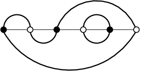
We first give the classic informal picture of a meander. Consider a river, oriented from west to east, with bridges. A meander is a closed, self-avoiding road which crosses all the bridges. A meandric system with roads is a set of non-intersecting meanders. A more formal definition is the following one.
Definition 3.
(Meanders and meandric systems). A meander of order is a closed, self-avoiding curve (the road) which crosses an infinite oriented horizontal line (the river) exactly times (the bridges). The number of meanders of order is denoted .
A meandric system of order with components is a set of non-crossing meanders all intersecting the same horizontal line, exactly times in total. The number of meandric systems with components and of order is denoted . Two systems are equivalent if there is a homeomorphism of the plane mapping one to the other.
Another representation of the problem of counting the number of meanders is the problem of calculating the entropy associated to compact foldings of a polymer on the plane [23, 28].
We will use the canonical representation, where the river is oriented from west to east, has marked vertices (black and white ones), the segments of the roads above and under the river are represented as semi-circular arches (caps and cups) whose feet are the vertices. An example is provided in the Figure 2.
II.1.2 Graphical re-encoding of Wick pairings
The contributions which dominate the large limit in the Equation (14) are the graphs such that the subgraphs with colors 0,1,2 and with colors 0,3,4 both have vanishing genus. As usual, this can be formulated as a planarity criterion. First, draw the face with colors as a convex -gon and the lines of color 0 on the exterior region, joining the vertices with labels and . The genus is zero if and only if this graph is planar. Then proceed similarly with the face with colors , which has to be ”unfolded”. Draw it as a convex -gon with vertex labels . Then the lines of color 0 connect to . Draw them on the exterior of the -gon. It comes that the genus vanishes if and only if this graph is planar.
The drawback of this representation is that we actually need two separate drawings in order to draw both the faces with colors and with colors as -gons. To improve the situation, we can draw the lines of color 0 inside the -gon with colors , which does not change the equivalence between planarity and vanishing genus. Then we can identify the two -gons, to get a single one, with edges of color 0 on the exterior, representing the permutation , and a copy of the Wick pairing on the inside representing the permutation . Finally we can cut the -gon and stretch it horizontally. This way we obtain a horizontal line with semi-circular arches on the upper half plane and on the lower half-plane.
In the following it will be useful to identify permutations with arch configurations.
Definition 4.
(Permutations and arch configurations). A permutation can be represented as a (most of the time non-planar) arch configuration on the set of ordered vertices , by ordering the vertices on a horizontal line, from left to right, and drawing arches between and , . The arches can be drawn all in the upper or lower half-plane. The other way around, any arch configuration gives rise to a permutation.
A permutation is said to be planar, , if its arch configuration is planar.
Step by step, our new representation of a Wick pairing on a graph is obtained in the following way.
- •
Draw a horizontal line with alternating black and white vertices which get the labels from west to east.
- •
The permutation is represented in the upper half-plane by semi-circular arches connecting to , . The genus vanishes if and only if the arch configuration is planar (note that this is however independent of and ).
- •
The permutation is represented in the lower half-plane by semi-circular arches connecting to , , and planarity of the arch configuration is equivalent to .
- •
We end up with two arch configurations, which form closed roads winding across a river. In the large limit, only the planar arch configurations survive, which are exactly meandric systems of order .
Proposition 3.
Let be the set of meandric systems such that if is the upper arch configuration, then is planar too and represents the lower arch configuration. We have thus shown that
| (19) |
In matrix model, graphs corresponding to the observables have a single face (with colors ) and by following the same reasoning as above, a Wick pairing is a permutation or equivalently an arch configuration. The number of planar permutations, describing a planar arch configuration, is the Catalan number and indeed the large evaluation
| (20) |
is very well-known. However, in our case, the presence of a second face, with colors , supported on the same set of vertices, makes the evaluation much more involved and explains the need for two arch configurations, and hence meandric systems in the large limit. Given and a planar upper arch configuration encoded by , the lower arch configuration, representing , is typically not planar…
This provides a very simple bound: the number of Wick pairings which contribute at large is bounded by the number of planar arch configurations,
| (21) |
II.2 Meandric permutations
Meandric systems can be described by permutations called meandric permutations [20]. First consider a labeling of the vertices of the horizontal line, say from left to right, , the odd vertices being the black ones and the even vertices being the white ones. The roads are also oriented such that they go from bottom to top at each black vertex. The meandric permutation is defined as a product of disjoint cycles, one for each road whose cycle is obtained by listing the vertex labels encountered along the road.
While there is a one-to-one correspondence between meandric systems and meandric permutations, it is very hard to identify the meandric permutations. A necessary condition is the following: if has cycles, then has cycles, of them on the odd labels and the others on the even labels .
It is easy to relate to our permutations .
Proposition 4.
Consider a meandric system in with as the upper arch configuration. Let denote the corresponding meandric permutation. Then
| (22) | ||||||
The proof simply tracks the labels along the oriented roads. It has the following interesting consequence.
Corollary 1.
A meandric system in with as the upper arch configuration has exactly closed curves, where denotes the number of cycles. In the case (respectively ), this reduces to (respectively ) and is therefore independent of the Wick pairing .
II.3 From meanders to Gaussian expectation values
We have shown that the expectation values of polynomials in a specific family can be evaluated as a number of meandric systems. We would also like to know whether while exploring the whole family of polynomials we encounter all meandric systems. It turns out to be the case, in the sense that from a meandric system and a given , it is possible to reconstruct a graph and a Wick pairing .
Proposition 5.
For any fixed , there is a one-to-one correspondence between meandric systems of order and elements of .
Proof. An element of is a meandric system characterized by (fixed), and an arch configuration . We thus have to show that there exist a unique and a unique for any meandric system. The vertices along the horizontal line are labeled from left to right, . By following the top arches we simply read : is the label of the black vertex connected to by an upper arch (see the Definition 4). We proceed similarly with the arches in the lower half-plane: is the label of the black vertex connected to by a lower arch. Since and are known, this defines . ∎
Corollary 2.
This immediately implies
| (23) | ||||||
| and | (24) |
(since the total number of meandric systems of order is the square of the Catalan number ).
III Factorization on stabilized-interval-free permutations
In this section we restrict attention to the case , and to simplify the notation we only write explicitly, like and so on.
In the trivial case we have
| (25) |
From the point of view of Wick’s theorem, the contributions come from the fact that the two 3-colored graphs formed by the all vertices and the edges of colors 0,1,2, and those of colors 0,3,4 are the same. Therefore the expectation value is the same as for a single-trace invariant in a Gaussian matrix model. In terms of meandric systems, this means that all the planar arch configurations on the upper half-plane are trivially reflected in the lower half-plane with respect to the horizontal line, by the trivial permutation on the vertices: the top and bottom arch configurations are the same. They correspond to all the meandric systems with exactly loops on vertices.
In the general case, we have the bound (21), but we would like to evaluate the expectation value exactly, or at least find a way to decompose it into smaller bits. As a first step, we will find a factorization onto expectation values of polynomials labeled by connected (or indecomposable) permutations [24]. Then we will use the cyclic permutation invariance to reduce the number of irreducible blocks to SIF permutations [21].
Definition 5.
(Decomposition into stabilized blocks). Let and . We say that decomposes into (stabilized) blocks if
| (26) |
i.e. stabilizes the intervals . A permutation which does not admit any block decomposition, except the trivial one (, ), is called a connected permutation.
Definition 6.
(Decomposition into connected blocks). Let and . We say that a block decomposition decomposes into connected blocks if it contains any other block decomposition as a subset, . If has a decomposition into connected blocks, the block permutations , defined as
| (27) |
are connected permutations.
The Definition 6 makes sense because when stabilizes two intervals, it also stabilizes their intersection. Therefore the decomposition into connected blocks is obtained as
| (28) |
and it is unique. In practice, it can be conveniently visualized using Murasaki diagrams [21].
We are interested in the set of meandric systems entering the Wick expansion of . When has a connected block decomposition , the set of (ordered) vertices on the horizontal line has a canonical decomposition into regions
| (29) |
When there is an upper arch which connects a white vertex to a black vertex , then there is a lower arch connecting the same white vertex to another black vertex in the same region (possibly itself if it is a fixed point of ).
There are meandric systems whose loops are each restricted to a single region and never visit two or more of them. Those meandric systems have the properties that simply cutting the horizontal line between each region, i.e. after each vertex , , reduces them to disconnected meandric systems. There is a subset of consisting of systems of this type,
| (30) |
The number of such systems is the product of the number of systems in each region where the permutation which relates the upper arch configuration to the lower configuration is . This implies the obvious bound
| (31) |
These meandric systems which get disconnected after one cut of horizontal line are called 1-reducible in [23].
The question is then whether there are really many more than the 1-reducible meandric systems of contributing to . The following Theorem shows that it barely is the case.
Theorem 1.
Let and such that decomposes into connected blocks and let be the corresponding connected permutations. Let denote the set of planar permutations on .
There is a bijective map between and , which implies
| (32) |
The proof proceeds with a few lemmas ; all the notations are borrowed from the Theorem 1.
Lemma 1.
There is an injective map .
Proof. We consider meandric systems in and glue them together so as to obtain a meandric system of order in , like in the Figure 3a. We label the vertices from left to right, so that are the vertices of the region .
Let be a planar permutation, like in the Figure 3b, which we are going to use to create a new meandric system in . All upper arches with a white vertex different from the last vertex of the region as a foot are left unchanged.


The remaining arches connect for each the white vertex to a black vertex . We cut them and rearrange them so that is now connected to , like in the Figure 3c. This new arch configuration is planar.
- •
Since we started from arch configurations each restricted to a region with as its last vertex, there is no arch going above the one between and , see the Figure 3a. Therefore when it is cut to create two new arches connected those vertices to other regions, the newly created arches do not cross any of the arches restricted to the regions .
- •
Since is planar, it induces a planar arch configuration for the newly created arches which therefore do not cross each other.
The upper arch configuration induces a lower configuration which for the same exact reasons is planar too.
Moreover, given an arch configuration with arches possibly connecting to other regions and all other arches connecting black to white vertices of the same region, we can reconstruct a unique element of . If is connected to a region , , there is a single black vertex also connected outside of . Then we cut those arches to connect to . This leads to a meandric system in . The permutation is found as the one which sends to the white vertex was initially connected to. ∎
It remains to show that the map introduced above is surjective.
Lemma 2.
Let be a connected permutation. Then,
| (33) |
Proof. If there exists such that for all , , then the interval is stabilized and is not connected. ∎
Lemma 3.
With the same hypotheses as in the Theorem 1, for each meandric system in and for each region , there is at most one upper arch which connects a white vertex of to a different region, and the white vertex can only be the last vertex of , .
Proof. Assume that there is an upper arch which connects , with , to a black vertex in a different region , . For definiteness, we assume that so that lies to the right of . Then there is also a lower arch which connects to a black vertex of ,
Applying the Lemma 2 to the restriction of to , it is found that there exists a black vertex with , whose image is on the left of , i.e. ,
Now we look for the white vertices which can be connected to via an upper arch.
- •
For planarity reason, there can be no upper arch between any white vertex on the left of and since it would cross the arch between and .
- •
Similarly, no upper arch can connect to any white vertex on the right of .
- •
If there is an upper arch between and a white vertex in , then there is a lower arch between this white vertex and which would cross the lower arch between and .
Therefore, the only possibility is to draw an upper arch between and a white vertex . To avoid a crossing in the lower plane, we further must have . Since both , we find that
| (34) | |||
i.e. is not the last white vertex of . The order of the so far relevant vertices is
| (36) |
Thanks to (34) we can apply the Lemma 2 to the restriction of to to get that
| (37) | |||
As it is clear from the picture, planarity requires that the white vertex connected to by an upper arch is in . This in turn gives rise to a lower arch between this white vertex and . This clearly breaks planarity in the lower plane,
Consequently, there can not be any upper arch connecting to another region. ∎
Proof of the Theorem 1. The Lemma 3 implies that all meandric systems in are also in the image of the map introduced in the Lemma 1 and its proof. Therefore this map is also surjective, which proves the Theorem 1. ∎
Thanks to the Theorem 1, we are left with the problem of determining the expectation values of polynomials labeled by connected permutations. This is however not helpful in the limit of large number of vertices since the number of connected permutations behave as , [21, 24]. Nevertheless, the Theorem 1 may still apply to some connected permutations, using the fact that a cyclic re-ordering of the labels does not change the expectation value while it can turn a connected permutation in a non-connected one. Eventually one is left with stabilized-interval-free permutations whose set of meandric systems actually corresponds to the set of 2-irreducible meandric systems.
Definition 7.
(Stabilized-Interval-Free permutations). We say that a permutation is stabilized-interval-free (SIF) if it does not stabilize any subinterval of , i.e.
| (39) |
except . We denote the set of SIF permutations.
Definition 8.
(2-Reducible and irreducible meandric systems.) We say that a meandric system is 1-reducible if a single cut on the horizontal line can produce two disconnected systems, and we say that it is 1-irreducible otherwise. A meandric system is said to be 2-reducible if it becomes disconnected after two cuts of the horizontal line, and 2-irreducible otherwise.
This notion was introduced in [22] (see also [23]). A 2-reducible meandric system has the structure of the Figure 4.

The Theorem 1 has the following extension.
Theorem 2.
The expectation value can be factorized as a product of Catalan numbers and expectation values of polynomials labeled by SIF permutations. The set is the set of 2-irreducible meandric systems.
Proof. Assume that has a connected block decomposition with block permutations . If all of them are SIF, there is nothing to prove. Assume that for some is connected but not SIF, which means there exists a stabilized interval . Then is not connected since it stabilizes . Furthermore this is just a cyclic shift of the labels induced by the face of colors , so that , hence the Theorem 1 applies to . We can do so until we are left with SIF permutations only.
The second part of the theorem states the equivalence between and 2-irreducible meandric systems. Consider a 2-reducible meandric system in . It contains a meandric system which can be disconnected by two cuts on the horizontal line, like in the Figure 4. This system either sits in a region which starts with a black vertex or with a white vertex . In both cases, the white vertices in that region are connected by upper arches to the black vertices of , and by lower arches to their images . Clearly this set is included in , and therefore stabilizes .
Reciprocally, consider a permutation which stabilizes . Thanks to a cyclic relabeling of the vertex labels, we can shift this interval to the left of the horizontal line, and work with which stabilizes (). is not connected, so there exist which decompose into connected blocks with permutations . There is such that and for simplicity we consider . The set can be described as , according to the Theorem 1. If is a fixed point of the planar permutation , it means that the meandric system from is contained in and no arch connects it to the other systems. This is obviously 1-reducible, and upon a cyclic relabeling, it typically becomes 2-reducible. Now we assume which means that the white vertex is connected outside . Consequently, there is another white vertex outside this region which has an upper arch and a lower arch connected in . This looks like
| (40) |
The colored area represent two regions with meandric systems which can not communicate. Clearly, the two vertical dashed lines indicate places where cuts can be performed and disconnect the full system into two pieces.
∎
SIF permutations do not allow fixed points and therefore form a subset of the derangements. Since the number of derangements grows like , this is an improvement with respect to the set of connected permutations. It turns out that the number of SIF permutations also grows like [21]. A more thorough study of SIF permutations will appear in a subsequent publication.
IV Applications and examples
IV.1 Applications of the theorems
We can use the Theorems 1 and 2 to calculate some expectation values easily, and in particular recover analytically the number of meandric systems with reasonably close to . The limitation is that we have to exhaust all the permutations on with exactly cycles before summing the corresponding expectation values.
Proposition 6.
The numbers of meandric systems of order with components are
| (41a) | ||||
| (41b) | ||||
| (41c) | ||||
Proof. Equation (41a). The only permutation with cycles is the identity whose connected block decomposition consists of blocks which are the identity on the 1-element sets , . The Theorem 1 gives the expected well-known answer .
Equation (41b). The permutations with exactly cycles are the transpositions , for . Since the expectation value is invariant under conjugation by the cyclic shift , we can consider the transposition between and instead. It has one connected block with cycle decomposition
| (42) |
and blocks which are the identity on , . The Theorem 1 gives
| (43) |
The expectation value for is the same as for the transposition between the first two elements, , for which the Theorem 1 yields , as for the transposition on two elements. Therefore
| (44) |
To perform the sum over all transpositions, we use a reasoning that we will later reproduce in more complicated situations. The sum over can be organized as a sum over the gap and a sum over the position of implemented using the conjugation by on , for ,
| (45) |
Here is a symmetry factor which corrects for the fact that each transposition appears twice in the orbit of under the action of (once with and once with ), hence . Moreover, since the action of leaves the expectation values invariant, there are equivalent positions for , which means that we can fix () and extract a factor . Thus,
| (46) |
Using the standard recursion , we get
| (47) |
Equation (41c). We distinguish three types of contributions to permutations with exactly cycles.
- 1.
has fixed points and transposes with and with , with a crossing, e.g. .
- 2.
has fixed points and transposes with and with , without crossing, e.g. .
- 3.
has fixed points and contains a 3-cycle . There are two orientations for the cycle, but both leads to the same expectation value.
The sum over is organized as a sum over the gaps and a sum over the position of implemented via the conjugation by , . Since a given permutation will appear times in an orbit ( and the three cyclic permutations on , e.g. ), the symmetry factor is . Conjugations by leave the expectation values invariant, meaning that there are equivalent positions for . Setting and factorizing we get
| (49) |
Using , then and , we arrive at
| (50) |
We therefore have to evaluate for ,
| (51) |
where the number of terms in the last sum is independent of . This finally leads to
| (52) |
Case 2. There are two typical patterns, one where the two transpositions are separated, e.g. , and the other where they are nested, e.g. . In the nested case we have
| (53) |
As before, we first keep the distances between the elements which are transposed fixed and sum over the position of using the orbit generated by . Notice that along an orbit one pattern can be turned into the other. This implies in particular that both patterns have the same expectation values. Therefore the symmetry factor is , where comes from the two patterns and from the number of times a permutation appears. We fix , extract a factor , and
| (54) |
The absolute positions of and are irrelevant and only the gap matters. There are possible positions for , hence (after the change )
| (55) |
In the final steps, the following formula for , is used several times,
| (56) | ||||
On the first line, we split the sum into two halves and relabel one of them , On the second line we factorized the common terms, and noticed in the third line that the sum which has a -dependent number of terms can be done. The number of terms in the remaining sums is independent of . A similar formula holds for . This allows to perform the sum over and then the sum over , to get
| (57) |
Case 3. The Theorem 1 provides the expectation values,
| (58) |
with . To sum over the permutations , we again sum over the positions of using the action of and over the gaps . The symmetry factor is . Therefore,
| (59) |
It is then straightforward to get
| (60) |
Finally,
| (61) |
leads to the conclusion. ∎
IV.2 Some expectation values for SIF permutations
In all cases the Theorems 1, 2 are applied, the Gaussian expectation values of polynomials labeled by SIF permutations are eventually needed. In the previous applications, they were permutations on very few elements (for ). Here we study a family of SIF permutations on an arbitrary number of elements.
Proposition 7.
Let be the cyclic permutation on . Then
| For | (62a) | |||||
| For | (62b) | |||||
| Other cases | (62c) | |||||
where and are the Catalan and Motzkin numbers of order .
Proof. Equation (62b). has a single cycle therefore the expectation value counts a number of meanders (a single component). For definiteness, we will only consider the case , so that the relevant meanders are such that there is an upper arch connecting to if and only if there is a lower arch connecting to .
We aim at a recursion on the degree of the polynomial and for the time of the proof we switch to the better adapted notation for .
Let and denote the number of contributing meanders with an upper arch between and . They also have a lower arch connecting to ,
Then we show that the upper arch with as a foot can only connect to . Indeed, first notice that due to planarity in the upper half plane, no vertex for can be connected to . Second, if , for , is connected to , then there is a lower arch which connects to and it clearly crosses the lower arch between and ,
Therefore there is an upper arch between and and a lower arch between and ,
It is then easy to see that the number of arch systems allowed in the region is precisely . Indeed, any meanders in of order can be inserted in the region by changing the lower arch connected to to an arch connected to instead, and this works the other way around. Similarly, the number of arch systems allowed in the region is . Consequently, for ,
| (63) |
For , it is even simpler to find
| (64) |
To get to , it only remains to sum over the position of ,
| (65) |
Together with the initial conditions , this recursion defines the Motzkin numbers and .
Equation (62c). Let . Our strategy is to prove that choosing completely determines a meandric system. The following lemma will be useful.
Lemma 4.
Let . If a meandric system in has an upper arch between and with and , then there is also an upper arch between and .
Proof of the Lemma. The meandric systems in are such that for every upper arch between and , there is a lower arch between and , and reciprocally.
Let with for the time being, and consider an upper arch between and , together with the lower arch between and ,
The drawing is made for , but everything works the same for with .
We are going to prove that there must be an upper arch between and . Assume that in the upper half plane is connected to , and to , with , , . In the lower half plane, they induce an arch between and , and an arch between and ,
Given that
| (66) |
we find that
| (67) |
Now we focus on the second case, ,
On the drawing, we have considered , but in the case , we have to use . It does not change the arguments below.
Notice that due to as well as , . Therefore there exists a vertex which is surrounded in the lower half plane by the arch between and and must be connected to via a lower arch,
In the upper half plane, is thus connected to . If , this is but this cannot be planar in the upper half-plane. So we are left with the case and an upper arch between and . However,
| (68) |
the second inequality being due to our starting assumption . As a result, the upper arch between and intersects the upper arch and ,
Therefore we must have and .
In the case , the Equation (68) gives , but is already so this is impossible. We can also look at this case directly. If , then , meaning that there is lower arch between and . This enforces a lower arch between and which can not have other partners. In the upper half-plane that new arch induces an arch between and which is the expected result. ∎
Back to the Equation (62c).
- •
The Lemma 4 directly applies to the cases with .
- •
When , we can simply flip the system with respect to the horizontal line, exchanging the upper and lower half-planes. This gives an upper arch between and and a lower arch between and . Since and , we can apply the Lemma 4 to the flipped meandric system with and .
- •
When and , by flipping the system again to exchange the upper and lower half-planes, we can work with the permutation instead of . Setting , the Lemma 4 applies since .
- •
The last case to analyze is . If , we can proceed just like for . If , there must be a lower arch between and which implies in the upper half-plane an arch between and . Then moving the pair of vertices to the far right of the horizontal line, we are again in position to apply the Lemma 4.
The result of this analysis is that once is chosen, there must be another arch in the upper half-plane (up to a flip of the system) below the initial one. This gives rise to a recursive process which fills a region, say (up to a redefinition of ), with arches on top of one another,
If is even, then we cyclically shift the vertices so that the pair becomes the leftmost pair on the horizontal line. Then the arch between and becomes an arch between the first white vertex and the last black vertex of the horizontal line,
which means that the above recursive process applies again, until all arches are determined.
If is odd, we cyclically shift the vertices so that the pair becomes the leftmost pair on the horizontal line. The same result is eventually obtained.
Since can take values, the expectation value is simply . ∎
Motzkin paths. It is well-known that planar arch configurations are one-to-one with Dyck paths. A Dyck path of order is a -step path in the upper half-plane which starts at , ends at and for which only two types of steps are allowed, the north-east step and the south-east step . Given an arch configuration over vertices on a horizontal line, oriented west to east, we list between each pair of consecutive vertices the number of arches which pass. This produces a list of positive integers which are interpreted as the heights of a Dyck path after the step .


Motzkin numbers are known to count Motzkin paths. A Motzkin path of length is a path of steps in the upper half-plane which starts at and ends at with three types of steps, north-east , south-east or east , i.e. the horizontal step.
Therefore it is interesting to find a bijection between and the set of Motzkin paths. Consider a meander in . Looking at a pair of vertices, there are four patterns which can arise the upper half-plane, displayed in the Figure 5. In terms of Dyck paths, they represent the four possible combinations of two successive steps: Figure 5a is two steps down, 5b two steps up, 5c one up and one down, and finally 5d one down and one up. However, meanders in can not contain the pattern 5d. Indeed, up to a cyclic permutation of the vertex labels, we can assume that we are looking at the leftmost pair of vertices . Then, they are either connected together like in the Figure 5c, or the white vertex is connected to some , . In this case, we know from the proof of Equation (62b) in the Proposition 7 that is connected by an upper arch to . Therefore when the labels are cyclically shifted, two arches always connect the pair to the two vertices of a pair (). Therefore these two arches always point in the same direction, like in the Figures 5a, 5b.
As a consequence, only three patterns in the upper-half plane are allowed. To find Motzkin paths, it is sufficient to just associate with the Figure 5a the south-east step, with 5b the north-east step and with 5c the horizontal step. The other way around it is straightforward to show that a Motzkin path gives rise to a single meander in .
Conclusion
We have shown in this paper that it is possible to perform calculations of expectation values beyond the so-called melonic sector in the Gaussian random tensor model. We have considered the family of polynomials in the tensor entries whose graphical representation possesses a single face with colors and a single face with colors . This generalizes the single-trace invariant of random matrix models to two faces superimposed on the same set of vertices instead of a single face. The expansion of their expectation value onto Feynman graphs is equivalent to a problem of enumeration of meandric systems whose lower and upper arch configurations are related by a permutation on the arch feet. The Theorems 1 and 2 reduce the difficulty to the evaluation on SIF permutations [21], which enumerate the irreducible meandric systems of [22] (see also [23]). In the Proposition 7 we have further evaluated the expectation values of polynomials labeled by some SIF permutations.
All the proofs of the paper use the meandric representation of the Feynman expansion which turns out very convenient. However, we want to stress that we could have used the set of Schwinger-Dyson Equations (SDE) instead. This is a set of equations that is derived from the integral expression (1) (see [27]) and generalizes the Tutte equation for the resummation of planar maps to Feynman amplitudes in quantum field theory. Those equations have already been used to solve tensor models at large in [19], and they also work in the present case. However, we have decided not to include the proofs using the SDE for two reasons: introducing them in the case of tensor models is space consuming, and the proofs would be quite redundant. Indeed, the SDE form an algebraic system on the expectation values of polynomials. Since it does not rely on the Feynman expansion, it seems at first that solving them does not involve any planarity requirement like the meandric representation. However, at large we can show that only the polynomials which maximize the number of connected components on the colors and contribute (the ”freeness” property) and this is actually equivalent to planarity of the Feynman graphs. Therefore proving our results using the SDE would consist in repeating the same arguments using ”maximal number of connected components of subgraphs” instead of ”planarity”.
Nevertheless, the question of going further than our results which rely on direct combinatorial analysis remains open and could benefit of the use of the SDE. A similar question is whether the Gaussian tensor model and its SDE can be useful to meander theory. It has been shown that random matrix models are useful to meanders [28]. As for random tensor models, we have shown that some simple results of meander theory can be recovered, like the Proposition 6. But it is far from clear that more advanced results can be reproduced, like those of [28, 29]. An important difference in our work is that we have enlarged the set of configurations from planar arch configurations to permutations. While this may be useful, it also means that most expectation values actually vanish since even after reduction by the Theorem 2, we are left with SIF permutations whose number grows like while the total number of meandric systems grows exponentially, . This is already a new piece of information for random tensor models. But it may be a drawback to progress in meander theory since it seems really difficult to find necessary and/or sufficient conditions on the permutation for an expectation value to vanish22 2 For instance, the polynomial labeled by (69) in cycle notation, has a vanishing large Gaussian expectation value. It satisfies the property (70) and similarly for all . But it is not a sufficient condition since the permutation also satisfies this property but has a non zero expectation..
Acknowledgements
Both authors are thankful to Perimeter Institute for Theoretical Physics which made this collaboration possible.
References
- [1] R. Gurau and J. P. Ryan, “Colored Tensor Models - a review,” SIGMA 8, 020 (2012) [arXiv:1109.4812 [hep-th]].
- [2] P. Di Francesco, P. H. Ginsparg and J. Zinn-Justin, “2-D Gravity and random matrices,” Phys. Rept. 254, 1 (1995) [arXiv:hep-th/9306153].
- [3] J. Ambjorn, B. Durhuus and T. Jonsson, “Three-Dimensional Simplicial Quantum Gravity And Generalized Matrix Models,” Mod. Phys. Lett. A 6, 1133 (1991).
- [4] N. Sasakura, “Tensor model for gravity and orientability of manifold,” Mod. Phys. Lett. A 6, 2613 (1991).
- [5] M. Gross, “Tensor models and simplicial quantum gravity in 2-D,” Nucl. Phys. Proc. Suppl. 25A, 144 (1992).
- [6]
A. Baratin and D. Oriti,
“Group field theory and simplicial gravity path integrals: A model for Holst-Plebanski gravity,”
Phys. Rev. D 85, 044003 (2012)
[arXiv:1111.5842 [hep-th]].
A. Baratin and D. Oriti, “Ten questions on Group Field Theory (and their tentative answers),” J. Phys. Conf. Ser. 360, 012002 (2012) [arXiv:1112.3270 [gr-qc]]. - [7]
R. Gurau,
“The 1/N expansion of colored tensor models,”
Annales Henri Poincare 12, 829 (2011)
[arXiv:1011.2726 [gr-qc]].
R. Gurau, “The complete 1/N expansion of colored tensor models in arbitrary dimension,” arXiv:1102.5759 [gr-qc]. - [8] V. Bonzom, R. Gurau and V. Rivasseau, “Random tensor models in the large N limit: Uncoloring the colored tensor models,” Phys. Rev. D 85, 084037 (2012) [arXiv:1202.3637 [hep-th]].
- [9] V. Bonzom, R. Gurau, A. Riello and V. Rivasseau, “Critical behavior of colored tensor models in the large N limit,” Nucl. Phys. B853, 174-195 (2011). [arXiv:1105.3122 [hep-th] ]
- [10]
J. Ben Geloun,
“Renormalizable Models in Rank Tensorial Group Field Theory,”
arXiv:1306.1201 [hep-th].
J. Ben Geloun, “Asymptotic Freedom of Rank 4 Tensor Group Field Theory,” arXiv:1210.5490 [hep-th].
J. Ben Geloun and D. O. Samary, “3D Tensor Field Theory: Renormalization and One-loop -functions,” Annales Henri Poincare 14, 1599 (2013) [arXiv:1201.0176 [hep-th]].
J. Ben Geloun and V. Rivasseau, Commun. Math. Phys. 318, 69 (2013) [arXiv:1111.4997 [hep-th]]. - [11]
V. Bonzom, R. Gurau and V. Rivasseau,
“The Ising Model on Random Lattices in Arbitrary Dimensions,”
Phys. Lett. B 711, 88 (2012)
[arXiv:1108.6269 [hep-th]].
V. Bonzom and H. Erbin, “Coupling of hard dimers to dynamical lattices via random tensors,” J. Stat. Mech. 1209 (2012) P09009. arXiv:1204.3798 [cond-mat.stat-mech].
V. Bonzom, “Multicritical tensor models and hard dimers on spherical random lattices,” Phys. Lett. A 377 (2013) 501-506 arXiv:1201.1931 [hep-th].
V. Bonzom and F. Combes, “Fully packed loops on random surfaces and the 1/N expansion of tensor models,” arXiv:1304.4152 [hep-th]. - [12] R. Gurau, “Universality for Random Tensors,” arXiv:1111.0519 [math.PR].
- [13] R. Gurau and J. P. Ryan, “Melons are branched polymers,” arXiv:1302.4386 [math-ph].
- [14] A. Tanasa, “Combinatorics of random tensor models,” Proceedings of the Romanian Academy A13 (2012) 27-31 [arXiv:1203.5304 [math.CO]].
- [15] V. Bonzom and R. Gurau, “Counting Line-Colored D-ary Trees,” arXiv:1206.4203 [math-ph].
- [16] R. Gurau and G. Schaeffer, “Regular colored graphs of positive degree,” arXiv:1307.5279 [math.CO].
- [17] S. Dartois, V. Rivasseau and A. Tanasa, “The 1/N expansion of multi-orientable random tensor models,” arXiv:1301.1535 [hep-th].
- [18] S. Dartois, R. Gurau and V. Rivasseau, “Double Scaling in Tensor Models with a Quartic Interaction,” JHEP 1309, 088 (2013) [arXiv:1307.5281 [hep-th]].
- [19] V. Bonzom, “Revisiting random tensor models at large N via the Schwinger-Dyson equations,” JHEP 1303 (2013) 160, arXiv:1208.6216 [hep-th].
- [20]
M. Lacroix,
“Approaches to the enumerative theory of meanders,”
http://www.math.uwaterloo.ca/~malacroi/Latex/Meanders.pdf - [21] D. Callan, “Counting stabilized-interval-free permutations,” arXiv:math/0310157 [math.CO].
- [22] S. Lando and A. Zvonkin, “Plane and Projective Meanders,” Theor. Comp. Science 117 (1993) 227-241.
- [23] P. Di Francesco, O. Golinelli and E. Guitter, “Meander, folding and arch statistics,” Math. Comput. Modelling 26N8, 97 (1997) [hep-th/9506030].
- [24] L. Comtet, “Advanced Combinatorics,” D. Reidel, Boston, 1974.
- [25] V. Bonzom, “New 1/N expansions in random tensor models,” JHEP 1306 (2013) 062, arXiv:1211.1657 [hep-th].
- [26] V. Bonzom and F. Combes, “Fully packed loops on random surfaces and the 1/N expansion of tensor models,” arXiv:1304.4152 [hep-th].
- [27] R. Gurau, “The Schwinger Dyson equations and the algebra of constraints of random tensor models at all orders,” Nucl. Phys. B 865, 133 (2012) [arXiv:1203.4965 [hep-th]].
- [28]
P. Di Francesco, O. Golinelli, E. Guitter,
“Meanders: Exact Asymptotics,”
Nucl. Phys. B 570 (2000) 699-712
arXiv:cond-mat/9910453v3.
P. Di Francesco, “Matrix model combinatorics: Applications to folding and coloring,” math-ph/9911002. - [29]
P. Di Francesco,
“Meander determinants,”
Commun. Math. Phys. 191, 543 (1998)
[hep-th/9612026].
P. Di Francesco, O. Golinelli and E. Guitter, “Meanders and the Temperley-Lieb algebra,” Commun. Math. Phys. 186, 1 (1997) [hep-th/9602025].