∎
Numerical resolution of algebraic equations with symmetriesThanks: This work has been supported by projects MTM2010-19510/MTM (MCIN), MTM2012-30860(MECC) and VA118A12-1 (JCYL).
Abstract
Studied here is the effect of the presence of symmetry groups in a system of algebraic equations on the numerical resolution with fixed-point algorithms. It is shown that the symmetries imply two important properties of the system: the solutions are not isolated, but distributed in orbits by the symmetry group and zero is an eigenvalue of the Jacobian evaluated at any of the solutions, being the multiplicity at least the dimension of the symmetry group. The use of the corresponding quotient space by the symmetry group motivates the concept of orbital convergence. This also establishes the conditions under which a fixed-point algorithm converges to some element of the orbit of a solution of the system. Two numerical examples illustrate these results.
Keywords:
Symmetry group of algebraic equations Fixed-point algorithms Orbital convergenceMSC
65H10 47H10 65N221 Introduction
The resolution of systems of algebraic equations with symmetry groups appears in the mathematical treatment of many models, [21, 24]. These groups consist of transformations that map solutions of the algebraic system into other solutions. Some consequences of the existence of such symmetry groups, from an analytical point of view, have been described in e. g. [24]. The main goal of this paper is discussing the influence of the symmetries in the numerical procedures to approximate the solutions of the system. This is surely a question that is more or less implicitly observed but, to our knowledge, not formally discussed, except in particular cases, [1]. The study is focused on fixed-point iteration algorithms.
From this numerical setting, two main points of discussion emerge. On the one hand, the formation of the corresponding orbits by the group is an obstacle to assume local uniqueness for the solutions of the system. (This is necessary for some classical local convergence results.) On the other hand, the symmetry group incorporates a zero eigenvalue in the Jacobian of the system at the solution, which implies the existence of the eigenvalue one in the iteration matrix of the corresponding iteration operator if a fixed-point system is considered. This property prevents the application of many results of convergence, [25, 26, 18, 14].
More specifically, the following points of the paper are emphasized:
- •
Because of the existence of a symmetry group in the system of algebraic equations, the solutions cannot be isolated, since any transformed solution by the symmetry group is also a solution. Therefore, this property forces to talk in terms of orbits of solutions (or orbits of fixed points in the case of a fixed-point system) instead of isolated solutions. Via this symmetry group and the corresponding partition of the space into orbits, the system of equations is associated to a reduced system, whose solutions consist of the orbits of the solutions of the original one.
- •
Several points of influence of the symmetry group on the iterative resolution of the system are analyzed. It is first shown that the infinitesimal generators of the group at any solution are eigenvectors of the corresponding Jacobian of the system, associated to the zero eigenvalue. (When the system is of fixed-point type, the infinitesimal generators are eigenvectors associated to the eigenvalue equals one of the corresponding iteration matrix.) When the associated eigenspace is spanned by these infinitesimal generators, the Jacobian can be interpreted in terms of the Jacobian of the reduced system at the corresponding orbit. The rest of the spectrum is preserved by the symmetry group action.
The main consequence, in the numerical resolution, is the concept of orbital convergence. This means local convergence to some element of the orbit of a solution of the system, that is, convergence modulo symmetries of the group. The iterative algorithms are analyzed in the reduced space for the orbit solutions of the reduced system, leading to the derivation of classical convergence results but in the orbital sense. The limit point may be estimated, in a first approximation, by the component of the initial iterate in the eigenspace associated to the eigenvalue equals one of the iteration matrix of the fixed-point iteration function.
The structure of the paper is as follows. In Section 2 the definition of a symmetry group of a system of algebraic equations, along with several related concepts, are reminded. The orbit of a point by the group, the infinitesimal generators and the reduced system by the symmetries are emphasized. Some properties of the spectrum of the Jacobian matrix of the system at a solution are described; in particular, the existence of the zero eigenvalue because of the symmetry group and the structure of the associated eigenspace. This information is used in Section 3, where fixed-point iterations for the numerical resolution of this kind of systems are analyzed. (Now, the zero eigenvalue becomes one for the iteration matrix of the corresponding iteration function. The reduction by symmetries preserves the rest of the spectrum of the iteration matrix.) Thus, from the introduction of the concept of orbital convergence, classical results, like the Contraction Mapping Theorem, can be stated in an orbital sense. The limit point is an element of the orbit of the fixed point and Section 3 is finished off with some remarks about the structure of the error and estimates on this limit point. Finally Section 4 is devoted to some numerical illustrations. Two examples are considered. The first system appears in the modelization of an -body problem and involves a one-parameter symmetry group of rotations. The second example concerns the numerical generation of traveling waves in nonlinear dispersive wave equations and takes the Bona-Smith system of Boussinesq equations as a case study.
2 Systems of algebraic equations with symmetries
2.1 Notation and preliminaries
For details related to the definitions and properties mentioned in this section, see e. g. [21, 24]. Throughout this paper, will stand for a domain in () and will denote a -parameter () Lie group of transformations
| (1) |
acting on . is assumed to satisfy the following conditions:
- (A1)
is Abelian, connected and global.
- (A2)
acts regularly on .
The second property in (A1) means that is connected when its structure of manifold is considered and excludes discrete groups in our study. On the other hand, the global action implies that each element is a diffeomorphism on . Finally, it is said that acts regularly if the associated orbits
| (2) |
are of the same dimension and for each one can find a neighborhood such that each orbit intersects in a pathwise connected subset. This property and the global action imply that the orbits (2) are regular dimensional submanifolds of .
The infinitesimal generators of (1) play a relevant role in the present paper. They are the vector fields
| (3) |
and provide a local representation of the group, in the sense that the flow associated to each vector field (3) is a one-parameter symmetry group and any element of (1) is locally a composition of these transformations. Note that under the previous hypotheses on , for each , the vectors are linearly independent and since is Abelian, these one-parameter subgroups commute.
Finally the action of (1) can generate the quotient space . This consists of identifying points that belong to the same orbit and consequently its elements are orbits in the original manifold . The hypotheses assumed on imply that the quotient space is a () dimensional manifold.
2.2 Symmetry groups of equations
Considered now are systems of algebraic equations on on the form
| (4) |
where is assumed to be on . In the sequel, an equivalent fixed point system
| (5) |
for some iteration function , will also be considered. The equivalence between (4) and (5) is understood in the sense that is a solution of (4) if and only if is a fixed point of (5), that is,
The group (1) is said to be a symmetry group of (4) if each element has the property of transforming solutions of (4) into solutions, that is, [24]
| (6) |
Equivalently, the symmetry group condition for (5) is
| (7) |
2.3 Reduced system
The presence of the symmetry group (1) has some consequences in the structure of (4) that are relevant for our analysis. Note first that differentiating (6) with respect to and evaluating at we obtain that if is a solution of (4) then
where stands for the Jacobian of at and the are given by (3). This means that is singular and the vectors belong to . Equivalently, using (7), the iteration matrix , corresponding to the fixed point system (5), admits as eigenvalue with the as eigenvectors.
The second consequence concerns the way the systems (4), (5) can be reduced in the quotient space . This can be described by using local coordinates, [24]. The hypotheses (A1), (A2) allow to construct, in some neighborhood of , a system of local coordinates for which the group corresponds to translations in the first variables,
This implies that, locally, the infinitesimal generators are the first vectors of the canonical basis in ,
where has all the components equals zero except the one in the -th position, which values one. Note then that the symmetry group condition implies that close to , the system (4) is independent of the first variables () and can be written in the form
| (8) | |||||
such that the first equations in (8) are functionally dependent on the remaining ones. This implies a reduction of the first variables and the characterization of (4) in terms of the variables and the last functionally independent equations, that make up the so-called reduced system.
In terms of the fixed point system (5) the reduction process means that near the fixed point (5) can be written in the form
| (9) | |||||
| (10) |
where (10) is a local representation of the reduced fixed point system and (9) is functionally dependent on (10).
2.3.1 Example
In some cases, this reduction can be described more explicitly. This is the case of the following system in :
| (11) |
where . System (11) is a particular case of the one considered in the example 1 of section 4. Some explanations about the related physical model will be then relegated to there, since here we are only interested in illustrating the reduction process. System (11) admits the group of rotations
as a symmetry group. In this case, the reduction can be carried out by using polar coordinates
Thus, in terms of the variables , where , the reduced system is of the form
3 Fixed-point algorithms
3.1 Structure of the iteration matrix
The reduced fixed point system will mainly determine the local behaviour of the corresponding fixed point iteration for (5). Note that due to the local reduced form (9), (10) and the hypotheses on , in a neighborhood of , the iteration matrix is similar to a block matrix of the form
where , stands for the identity matrix and denotes the Jacobian of with respect to the variables at for . Consequently, the spectrum of the iteration matrix consists of the eigenvalue , associated to the presence of the symmetry group and the spectrum of the iteration matrix of the reduced fixed point system at the orbit of . In particular (see also [16]),
Lemma 1
Assume the hypotheses (A1), (A2). If is not an eigenvalue of the iteration matrix of the reduced fixed point system at the orbit of , then the geometric and algebraic multiplicities of as eigenvalue of equals with the vectors in (3) forming a basis.
3.2 Orbital convergence
The previous results are oriented to analyze the influence of the symmetries in the numerical resolution of (4) with the fixed-point iteration
| (12) |
and given initial data .
The concept of orbital convergence is now introduced. If is a solution of (4), the iteration (12) is said to be orbitally convergent to if there are a neighborhood of and such that if then , defined by (12), converges to . That is, orbital convergence means that the iteration converges locally to some element of the orbit of by the symmetry group (1).
Orbital convergence looks to be the natural concept to treat the convergence for this kind of problems, since this must be understood in the quotient manifold . The structure of the iteration matrix , previously described, clarifies the procedure to obtain results on orbital convergence, since the spectrum of the iteration matrix of the reduced system at the orbit of coincides with the part of the spectrum of which is not associated to the symmetry group. For instance, the Contraction Mapping Theorem, applied to the reduced system, leads to the following result (see also [1]).
3.3 Structure of the error
The structure of the iteration errors suggests an estimate, at first order, of the element of the orbit of to which the iteration converges. Let us assume that Theorem 3.1 holds. Let and suppose that the initial error satisfies . By using the spectrum of , we can decompose
for some . The term is the component of in the supplementary subspace of Ker in , consisting of the other invariant generalized eigenspaces associated to the eigenvalues different from . On the other hand, the second term of the error sequence can be written in the form
where . If we assume that , [30, 13, 14, 8], then can be written
where . Therefore, the second iterate is of the form
with . The previous arguments can be applied to a general step. We assume that
with . Then . Now
where . Now, if , then can be written
where . Therefore, the general -th iterate is
with . Thus, at order, approximates the element , associated to the projection of the initial iteration onto Ker, plus a term that, according to Theorem 3.1, converges to zero.
4 Numerical experiments
The previous results are illustrated by two examples.
4.1 Example 1. A -body problem
Given , and
we consider the system
| (13) |
where is a diagonal matrix with the indicated diagonal elements, with and
| (14) |
System (13), (14) appears in the modelization of the -body problem, where stands for the position of the -th body with mass (assuming a planar configuration) and where denotes a central mass, which is supposed to be at the origin, [2]. (The example considered in section 2 is a particular case with . This will be used again in the numerical experiments below.) In the case of (13), the solutions correspond to a configuration where bodies form regular polygons around the mass , see Figure 1. Assuming for simplicity that , a solution of (13), (14) is of the form, [23]
| (15) |
The dynamics of the corresponding solution of the -body system with initial data given by corresponds to a uniform rotation around with angular velocity given by , [9].


System (13), (14) admits the symmetry group of rotations (see Figure 2)
| (16) |
where, for , ,
| (17) |
The infinitesimal generator of the group is
| (18) |

By way of first illustration of the orbital convergence, an iterative method for (13), (14) is implemented with the goal of approximating the exact solution (15) and its corresponding orbit. Note that system (13) can be written in the form (5) with
| (19) |
Observe that is an homogeneous function of with degree . In particular, this implies that
and therefore is an eigenvalue of the iteration matrix . This means that the fixed-point algorithm with iteration function will not be convergent in general. A typical alternative for this kind of homogeneous systems is the so-called Petviashvili method. This method was originated in the context of the generation of lump solitary waves in the KP-I equation, [29], and it is widely used in this context, where nonlinearities with homogeneous functions are frequent. The application of the method to (13), (14) is as follows. From , a sequence of approximations to is generated by the formulas
| (20) | |||||
| (21) |
where is a free parameter and stands for the Euclidean inner product in . The analysis of the method has been carried out in several papers and for some cases [28, 20]. Essentially, local convergence, in both the classical and orbital sense, is obtained when is simple and is the only eigenvalue of with modulus greater than one and is chosen under the condition , with the best rate of convergence when . The arguments to obtain this result rely on the effect of the so-called stabilizing factor (20) on the spectrum of . This factor acts like a filter, eliminating the direction of divergence provided by the eigenspace associated to , [1]. Thus, the Jacobian of the iteration function of the procedure (20), (21) at the fixed point shares the spectrum of except the ‘harmful’ (from the point of view of the convergence) eigenvalue , which is transformed to an eigenvalue with modulus below one (eventually zero in the case ).
The procedure (20), (21) is written as a fixed-point algorithm with iteration function given by . It will be considered to illustrate the orbital convergence for the system (13), (14). First, and according to the previous comments, the convergence can be checked from Tables 1 and 2. For , , and several values of , these tables display, respectively, the eigenvalues of and of the iteration matrix , evaluated at the exact given by (15).
| -2.0000E+00 | -2.0000E+00 | -2.0000E+00 | -2.0000E+00 | -2.0000E+00 |
| 9.9999E-01 | 1.0000E+00 | 1.0000E+00 | -1.6000E+00 | -2.0000E+00 |
| -5.7143E-01 | -8.8888E-01 | -1.0000E+00 | 1.0000+00 | 1.0000E+00 |
| 2.8571E-01 | 4.4444E-01 | 5.0001E-01 | 8.0000E-01 | 1.0000E+00 |
| 9.9999E-01 | 1.0000E+00 | 1.0000E+00 | -1.6000E+00 | -2.0000E+00 |
| -5.7143E-01 | -8.8888E-01 | -1.0000E+00 | 1.0000+00 | 1.0000E+00 |
| 2.8571E-01 | 4.4444E-01 | 5.0000E-01 | 8.0000E-01 | 1.0000E+00 |
| 2.2205E-16 | 5.5511E-17 | -5.5511E-16 | 0 | 0 |
In the case of Table 1, the degree of homogeneity appears as simple, dominant eigenvalue, as well as , also simple. This last one corresponds to the symmetry group of rotations (16), (17). The effect of the method (20), (21) on the spectrum of the iteration matrix is observed in Table 2. The eigenvalue is filtered and becomes zero in the spectrum of the new matrix, while the rest of the eigenvalues is preserved.
Convergence is now discussed. According to the parameter , the following results include two convergent cases (), one not convergent case () and two divergent cases (). The convergent case is illustrated in Figure 3 , where the initial iteration is a perturbation of of the form
| (22) |
with and is the vector of ones of length . The procedure (20), (21) is run until one of the following errors is below a tolerance :
- (i)
- (ii)
The (relative) error with respect to the exact fixed point (15)
(24)
In both cases, the Euclidean norm is used and the errors are displayed in logarithmic scale and as functions of the number of iterations. Figures 3 (a) and (b) show (23) and (24), respectively, for the case while Figures 3 (c) and (d) correspond to . We observe that the larger the faster the iteration converges. The behaviour of the residual error (23) shows the convergence of the iteration. On the other hand, the errors (24), in both cases, stop decreasing from a certain iteration. This may indicate that this convergence is probably to an element of the orbit of , different from it and generated by a small component, in the initial iteration, associated to the eigenspace of the eigenvalue .


The linear order of convergence is confirmed in Figure 4, where the ratios are displayed as function of the number of iterations. As grows, the quotients tend to one.

The orbital convergence and the dependence on the initial iteration are also illustrated in Figures 5(a) and (b). Figure 5(a) displays the position of the fixed point (with filled circles) and of three final iterates of the algorithm (20), (21) obtained from initial iterations of the form
| (25) |
where is given by (18) and for (with squares), (diamonds) and (triangles). The fixed mass is . Since is the infinitesimal generator of the symmetry group (16), the different choices (25) reflect the influence of on the limit of the iteration, which in the three cases belongs to the orbit of by the symmetry group. This orbital convergence is also observed in Figure 5(b), which shows the final iterates obtained from initial iterations of the form (22) where (with squares), (diamonds) and (triangles).


The behaviour of the stabilizing factor (20), for several situations, is illustrated in Figure 6. Note that (20), when evaluated at the fixed point , is equal to one. Thus, in the case of convergence, the factors must tend to one. This is observed in Figure 6(a), that shows the discrepancy as function of the number of iterations and for the case . A different behaviour of the sequence of stabilizing factors indicates nonconvergence of (21). For example, the behaviour in Figure 6(b), corresponding to , may be justified by the presence, in the initial iteration (22), of a relevant component in the direction of the eigenspace associated to the eigenvalue (see Tables 1 and 2, third column). Note that the eigenvalue does not affect the behaviour of the stabilizing factor, since the quotient in (20) equals one at any element of the orbit of . Finally, the divergence in Figures 6 (c) and (d) occurs because of different reasons, see Tables 1 and 2, fourth and fifth columns. In the first case, there is an additional eigenvalue of modulus greater than one and different from ; in the second case, the dominant eigenvalue is not simple. This last situation corresponds somehow to a different model. When , the system is affected by forces which are inversely proportional to the distance between the bodies, see (14). Its inclusion, however, illustrates a different divergent situation. Note also the presence of a double eigenvalue .
4.2 Example 2. Traveling wave generation
The second example involves the translational symmetry with the numerical generation of solitary-wave solutions of the Bona-Smith system [3, 4, 6, 5]
| (26) |
for , with initial conditions
and
System (26) is a particular case of the family of Boussinesq systems considered in water wave theory, introduced in [3, 4]. It is an approximation to the two-dimensional Euler equations for the irrotational free surface flow of an incompressible, inviscid fluid in a uniform, horizontal channel, when no cross channel variations are considered. The variable is proportional to the position along the channel, is the time variable, while represent the deviation of the free surface from its undisturbed level at and the horizontal velocity of the fluid at , respectively, see [3, 4] for details.
One of the relevant properties of (26) is the existence of solitary-wave solutions. They are solutions of traveling-wave form with constant speed . The resulting waves are smooth, positive, even and decay to zero at infinity. By substitution into (26) and after one integration, the profiles must satisfy the system
| (27) |
where stands for the second order differentiation operator. System (27) admits the group of spatial translations
| (28) |
as symmetry group. On the other hand, existence of these solutions is established from [31], (see also [15]) for , although only in some cases analytical expression for the solitary waves is known [11]. Thus, for a typical value of , the profiles must be approximated by numerical means.
In order to treat (27) numerically, considered here is the corresponding periodic problem on a sufficiently long interval . Then, (27) is discretized by using a Fourier collocation method, [7]. This leads to the discrete system
| (29) |
where:
- •
stands for the identity matrix and is the pseudospectral differentiation matrix, [10].
- •
are vector approximations to at the collocation points .
Note that (29) inherits a symmetry group, infinitesimally generated by the vector field ,
which can be considered as a discrete version of (28), see the examples below. For fixed , an iterative technique can be applied to (29) in order to obtain the approximations . This has been carried out by using the Newton’s method
| (30) | |||||
| (31) |
(where ). (The previously described Petviashvili method could also being applied.) Note that since is singular, system (30) may be ill-conditioned. Two techniques for the resolution have been considered. The first one obtains that minimizes the Euclidean norm of the residual by using the minimum residual algorithm MINRES, [27]. The method is implemented in physical space, by computing in (29) and the Jacobian
| (32) |
at each iteration. (Note that the Jacobian is symmetric.) The second technique also makes use of the symmetry of (32) and solves (30) with preconditioned conjugate gradient (PCG) techniques, [17, 22]. Although the PCG method can be initially applied to the symmetric, positive definite case, it also may be implemented when the matrix is symmetric but indefinite, [12, 32]. In this case the implementation of the Newton’s method is carried out in Fourier space and involves two iteration loops: an inner iteration corresponding to the resolution of (30) with (PCG) and the outer iteration associated to the advance (31), [19, 20, 32]. On the other hand, a discrete version of preconditioning operators of the form
| (33) |
is used, where is a positive parameter to be adjusted according to the problem under implementation. The operators (33) are usually considered for this kind of problems, [32, 33]. The resulting method, consisting of the Newton’s method (30), (31) along with PCG for (30) will be denoted by (PCGN).
Both techniques have been performed and compared in terms of the behaviour of the residual error
| (34) |
in the Euclidean norm, when is given by (29). This error and the corresponding iteration are controlled by a fixed tolerance .
Our experiments show that both methods are comparable in efficiency with respect to the number of iterations, but the second one (PCGN) provides a higher performance in terms of the computational time. Then the results presented here correspond to this second procedure.
We first compare the numerical results with an exact profile. As mentioned before, analytical expressions for solitary wave solutions of (27) and fixed are in general unknown. However, some profiles can be found in closed form. For example, [11], for each , there is one solitary wave solution of the form
| (35) |
where is arbitrary (it is the translational parameter; associated to the symmetry group) and the rest of the parameters is given by


Figure 7(a) shows the spectrum of the Jacobian (32) at the exact profiles (35) with (evaluated at the Fourier collocation points; the size of the matrix is ). The indefinite character is observed and the magnification given by Figure 7(b) reveals the simple eigenvalue , associated to the translational symmetry of (29).


The results of the method are first compared with the exact profiles in Figure 8(a). This shows the behaviour of the error between the iteration and the profiles
| (36) |
in logarithmic scale and as function of the number of iterations. (The Euclidean norm is considered.) The initial iteration is a perturbation of the exact profiles of the form
| (37) |
with . The local convergence of the method is illustrated. On the other hand, the order of this convergence is displayed in Figure 8(b). This shows the ratios , also as function of the number of iterations. These ratios are bounded with , suggesting a linear convergenceand they look to rule out the convergence, [13, 14].


The orbital convergence is illustrated by the following figures. Figure 9(b) shows the final approximate profiles obtained by the (PCGN) method, with initial iteration displayed in Figure 9(a). This is of the form (37) with . The initial profiles are centered at the origin, and the displacement from it of the final iterates are computed as , so they can be considered as centered at the origin as well.
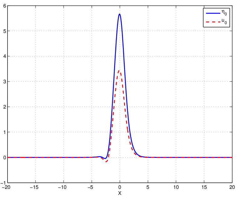

The effect of the translational symmetry is observed in Figure 10. From a profile of the form
| (38) |
with and , shown in Figure 10(a), the procedure converges (up to the fixed tolerance ) with the final iterates shown in Figure 10(b). The profiles are affected by a phase shift and centered at
(The computed coincide up to ten digits.)
| 1E-01 | -9.9534E-02 | -9.9534E-02 |
| 5E-02 | -4.9941E-02 | -4.9941E-02 |
| 1E-02 | -9.9995E-03 | -9.9995E-03 |
| 5E-03 | -4.9999E-03 | -4.9999E-03 |
A final experiment, related to the profiles (35), checks the local convergence and the effect of the components of the initial iteration associated to the symmetry on the limit profile. Initial iterations of the form
| (39) |
and several (small) values of , the phase shift of the final iterates have been computed and are shown in Table 3. The resulting displacements correspond, as decreases, to the limit profile associated to a spatial translation of .


A second group of experiments checks the accuracy of the method to approximate solitary wave profile solutions of (27) for which explicit formulas are not known. We have taken and two speeds, . By using as initial iterations the profiles (35) with , the final iterates are shown in Figure 11. For the first speed, Figure 11(a), the profiles are displaced with a phase shift (the same, up to ten digits, for both and ) of , while for the waves of Figure 11(b), corresponding to the second value of the speed, the computed phase shift, for both components, is below the machine precision, therefore no displacement is assumed.

The accuracy of the computed waves is checked in Figures 12 and 13. Figure 12 shows the residual error (34) as function of the number of iterations and in logarithmic scale, for the computed profiles displayed in Figure 11. As is known, (34) measures the error generated by the iterations in the formula (29) for the profiles. The method gets a residual error of order of about in less iterations in the case than for . (The number of iterations depends, among others, on the preconditioning parameter in (33). An optimal value of it may be different for different speeds.)


Finally, a necessary test to check the accuracy of the computed profiles as solitary wave solutions of the Bona-Smith system (26) consists of taking them as initial conditions of a code to integrate (26) numerically. Figure 13 illustrates the evolution of the solution, by displaying the form of the corresponding approximation at different times. (The experiment corresponds to .) A propagation without backward or forward disturbances is observed, a solitary wave-like evolution to the right with speed .
References
- (1) J. Alvarez, A. Duran, The Petviashvili method and its applications: I. Analysis of convergence, J. Comput. Appl. Math. (2014),http://dx.doi.org/10.1016/j.cam.2014.01.015.
- (2) Arnold, V.I.: Mathematical Methods of Classical Mechanics, Springer, Berlin (1989)
- (3) Bona, J.L., Chen, M., Saut, J.-C.: Boussinesq equations and other systems for small-amplitude long waves in nonlinear dispersive media: I. Derivation and linear theory, J. Nonlin. Sci. 12, 283-318 (2002)
- (4) Bona, J.L., Chen, M., Saut, J.-C.: Boussinesq equations and other systems for small-amplitude long waves in nonlinear dispersive media: II. The nonlinear theory, Nonlinearity 17, 925-952 (2004)
- (5) Bona, J.L., Smith, R.: A model for the two-way propagation of water waves in a channel. Math. Proc. Camb. Philos. Soc., 79, 167-182 (1976)
- (6) Boussinesq, J.V.: Théorie des ondes et des remous qui se propagent le long d’un canal rectangulaire horizontal, en communiquant au liquide contenu dans ce canal des vitesses sensiblement pareilles de la surface au fond, J. Math. Pures Appl. 17, 55-108 (1872)
- (7) Boyd, J.P.: Chebyshev and Fourier Spectral Methods, 2nd ed. Dover Publications, New York (2000)
- (8) Brezinski, C.: A classification of quasi–Newton methods. Numer. Algorithms, 33, 123–135. (2003)
- (9) Cano, B., Duran, A.: A technique to improve the error propagation when integrating relative equilibria, BIT 44, 215-235 (2004)
- (10) Canuto, C., Hussaini, M.Y., Quarteroni, A., Zang, T.A.: Spectral Methods in Fluid Dynamics, Springer-Verlag, New York-Heidelberg-Berlin (1988)
- (11) Chen, M.: Exact traveling-wave solutions to bi-directional wave equations. Int. J. Theor. Phys. 37, 1547-1567 (1998)
- (12) Demmel, J.: Applied Numerical Linear Algebra, SIAM Philadelphia (1997)
- (13) Dennis Jr., J.E., Moré, J.J: A characterization of super-linear convergence and its application to quasi-Newton methods, Math. Comput. 28, 549-560 (1974)
- (14) Dennis Jr., J.E., Moré, J.J: Quasi-Newton methods, motivation and theory, SIAM Rev. 19, 46-89 (1977)
- (15) Dougalis, V.A., Mitsotakis, D.E.: Solitary waves of the Bona-Smith system. In D. Fotiadis and C. Massalas, editors, Advances in Scattering Theory and Biomedical Engineering, pages 286-294. World Scientific, River Edge (2004)
- (16) Durán, A., Sanz-Serna, J.M.: The numerical integration of relative equilibrium solutions. Geometric theory, Nonlinearity 11, 1547-1567 (1998)
- (17) Golub, G.H., Van Loan, Ch.F.: Matrix Computations, J. H. U. Press, Baltimore (1996)
- (18) Griewank, A.: On solving nonlinear equations with simple singularities or nearly singular solutions, SIAM Rev. 27, 537-563 (1985)
- (19) Lakoba, T.I.: Conjugate Gradient method for finding fundamental solitary waves, Physica D 238, 2308-2330 (2009)
- (20) Lakoba, T.I., Yang, J.: A generalized Petviashvili method for scalar and vector Hamiltonian equations with arbitrary form of nonlinearity, J. Comput. Phys. 226, 1668-1692 (2007)
- (21) Marsden, J.E., Ratiu, T.S.: Introduction to Mechanics and Symmetry, Springer, New York (1994)
- (22) Meyer, C.D.: Matrix Analysis and Applied Linear Algebra, SIAM Philadelphia (2000)
- (23) Moeckel, R.: Linear stability analysis of some symmetrical classes of relative equilibria, in Hamiltonian Dynamical Systems, H. S. Dumas, K. R. Meyer and D. S. Schmidt, eds., Springer, New York, 291-317 (1995)
- (24) Olver, P.J.: Applications of Lie Groups to Differential Equations, Springer, New York (1986)
- (25) Ortega, J.M., Rheinbolt, W.C.: Iterative Solution on Nonlinear Equations in Several Variables, Academic Press, New York (1970)
- (26) Ostrowsky, A.M.: Solutions of Equations and Systems of Equations, Academic Press, New York (1966)
- (27) Paige, C.C., Saunders, M.A.: Solution of sparse indefinite systems of linear equations, SIAM. J. Numer. Anal. 12, 617-629 (1975)
- (28) Pelinovsky, D.E., Stepanyants, Y.A.: Convergence of Petviashvili’s iteration method for numerical approximation of stationary solutions of nonlinear wave equations, SIAM J. Numer. Anal. 42, 1110-1127 (2004)
- (29) Petviashvili, V.I.: Equation of an extraordinary soliton, Soviet J. Plasma Phys. 2, 257-258 (1976)
- (30) Stoer, J., Burlisch, R.: Introduction to Numerical Analysis, Springer-Verlag, New York (1983)
- (31) Toland, J.F.: Uniqueness and a priori bounds for certain homoclinic orbits of a Boussinesq system modelling solitary water waves, Commun. Math. Phys. 94, 239-254 (1984)
- (32) Yang, J.: Newton-conjugate-gradient methods for solitary wave computations, J. Comput. Phys. 228, 7007-7024 (2009)
- (33) Yang, J.: Nonlinear Waves in Integrable and Nonintegrable Systems, SIAM, Philadelphia (2010)