跳到论文正文
W Papers独立论文阅读器 arXiv:1310.3315 论文正文 计算阅读时间 · 0%
引用这篇论文根据当前论文元数据生成,正式投稿前建议核对。


License: arXiv.org perpetual non-exclusive license
arXiv:1310.3315v5 [hep-ph] 29 Aug 2017

Phenomenological Aspects of a TeV Scale Alternative left-right Model

M. Ashry1,2 and S. Khalil2,3 Affiliation: 1Department of Mathematics, Faculty of Science, Cairo University, 12613, Giza, Egypt.
2Center for Fundamental Physics, Zewail City of Science and Technology, Sheikh Zayed, 12588, Giza, Egypt.
3Department of Mathematics, Faculty of Science, Ain Shams University, 11566, Cairo, Egypt.
Abstract

We revisit the alternative left-right symmetric model, motivated by the superstring-inspired E6E_{6} model. We systematically analyze the constraints imposed by theoretical and experimental bounds on the parameter space of this class of models. We perform a comprehensive analysis of the Higgs sector and show that three neutral C​PCP-even and two C​PCP-odd Higgs bosons in addition to two charged Higgs bosons can be light, of 𝒪⁡(100){\cal O}(100) GeV. We emphasize that the predictions of this model for the signal strengths of Higgs decays are consistent with the standard model expectations. We also explore discovery signatures of the exotic down-type quark, which is one of the salient predictions of this model.

I Introduction

The discovery of neutrino masses and oscillations confirmed the fact that although the standard model (SM) is extremely accurate, it is still incomplete. The left-right Model (LRM) is the most natural extension of the SM that accounts for the measured neutrino masses and provides an elegant understanding for the origin of the parity violation in low-energy weak interactions [1, 2, 3, 4, 5, 6, 7, 8]. The LRM is based on the gauge group S​U​(3)C×S​U​(2)L×S​U​(2)R×U​(1)(B−L)/2×PSU(3)_{C}\times SU(2)_{L}\times SU(2)_{R}\times U(1)_{(B-L)/2}\times P, where PP is the discrete parity symmetry. In the LRM, standard model fermions are assigned in the following left- or right-handed doublets:

QL≡(uLdL),ψL≡(νLeL)&QR≡(uRdR),ψR≡(νReR).Q_{L}\equiv\left(\begin{array}[]{c}u_{L}\\ d_{L}\end{array}\right),~\psi_{L}\equiv\left(\begin{array}[]{c}\nu_{L}\\ e_{L}\end{array}\right)~~~\&~~~Q_{R}\equiv\left(\begin{array}[]{c}u_{R}\\ d_{R}\end{array}\right),~\psi_{R}\equiv\left(\begin{array}[]{c}\nu_{R}\\ e_{R}\end{array}\right). (1)

The parity symmetry: QL,ψL↔QR,ψRQ_{L},\psi_{L}\leftrightarrow Q_{R},\psi_{R} implies that the gauge couplings of left- and right-handed S​U​(2)SU(2) are equal, i.e., gL=gR≡gg_{L}=g_{R}\equiv g.

The Higgs sector of the LRM consists of (i)(i) bidoublet Φ⁡(1,2,2∗,0)\Phi(1,2,2^{*},0), which is required to construct the SM Yukawa couplings of quarks and leptons. (i​i)(ii) two scalar triplets ΔL​(1,3,0,2)\Delta_{L}(1,3,0,2) and ΔR​(1,0,3,2)\Delta_{R}(1,0,3,2) that break U​(1)(B−L)/2U(1)_{(B-L)/2} and generate neutrino Majorana masses. At high-energy scale, well above the electroweak breaking scale, the S​U​(2)R×U​(1)(B−L)/2×PSU(2)_{R}\times U(1)_{(B-L)/2}\times P symmetry is broken down to U​(1)YU(1)_{Y} by the vacuum expectation value (vev) of the neutral component of ΔR\Delta_{R}, and hence the right-handed Majorana neutrino mass is generated. In this type of models, the hypercharge YY is defined as Y=T3​R+(B−L)/2Y=T_{3R}+(B-L)/2, where T3​RT_{3R} is the third component of the right-handed isospin. At lower energy scales, Φ\Phi and ΔL\Delta_{L} acquire vevs that break S​U​(2)L×U​(1)YSU(2)_{L}\times U(1)_{Y} down to U​(1)e​mU(1)_{em}. It is worth mentioning that in the conventional LRM, one gets the following estimate for the associated vevs: ⟨ΔL⟩=vL​<∼​𝒪​(1)\langle\Delta_{L}\rangle=v_{L}\raise 1.29167pt\hbox{$\;<$\kern-7.5pt\raise-4.73611pt\hbox{$\sim\;$}}{\cal O}(1) GeV, ⟨ΔR⟩=vR​>∼​𝒪​(1011)\langle\Delta_{R}\rangle=v_{R}\raise 1.29167pt\hbox{$\;>$\kern-7.5pt\raise-4.73611pt\hbox{$\sim\;$}}{\cal O}(10^{11}) GeV, and ⟨Φ⟩=diag⁡{κ,κ′}\langle\Phi\rangle={\rm diag}\{\kappa,\kappa^{\prime}\} with κ′≪κ\kappa^{\prime}\ll\kappa and κ∼𝒪⁡(100)\kappa\sim{\cal O}(100) GeV [1, 3, 4].

It turns out that the Higgs sector of the LRM, in particular the Higgs triplets, may induce tree-level flavor-violating processes that contradict the current experimental limits. Therefore, it is usually assumed that S​U​(2)R×U​(1)(B−L)/2SU(2)_{R}\times U(1)_{(B-L)/2} is broken at a very high-energy scale. In this case, it is not possible to detect any residual effect for S​U​(2)RSU(2)_{R} gauge symmetry at the TeV scale in the Large Hadron Collider (LHC). This has motivated Ernest Ma, in his pioneering work in 1987 [9], to study variants of the conventional LRM. He has shown that the superstring-inspired E6E_{6} model may lead to two types of left-right models. The first one is the canonical LRM, while the second one is what is known as the alternative left-right Model (ALRM) [10, 11], where the fermion assignments are different from those in the conventional LRM in the following: (i)(i) an extra quark, dR′d^{\prime}_{R}, instead of dRd_{R}, is combined with uRu_{R} and form S​U​(2)RSU(2)_{R} doublet, and(i​i)(ii) an extra lepton, nRn_{R}, instead of νR\nu_{R}, is combined with eRe_{R} and forms S​U​(2)RSU(2)_{R} doublet. Therefore, the right-handed neutrino νR\nu_{R} is a true singlet and is no longer a part of the right-handed doublet.

It is remarkable that E6E_{6} is a complex Lie group of rank 6. It includes the S​O​(10)SO(10) group, so it is a good candidate for grand unification. Some string theories (Heterotic string) predict that the low-energy effective model is symmetric under E6E_{6}. Depending on the string model, E6E_{6} may be broken to S​O​(10)SO(10) and then to the conventional left-right model or it may have another branch of symmetry breaking that leads to the alternative left-right model that we consider. The particle content of the ALRM, derived from E6E_{6} model, contains more particles than those in the conventional LRM obtained from S​O​(10)SO(10). This can be simply understood from the fact that the fundamental representation 2727 of E6E_{6} is equivalent to the fundamental representation 1616 of S​O​(10)SO(10) plus its 1010 and singlet representations. In the conventional LRM, all non-SM particles are decoupled and can be quite heavy. However, in the ALRM, they are involved with the SM fermions and will have low-energy consequences. Furthermore, another important difference between the ALRM and the conventional LRM is the fact that tree-level flavor-changing neutral currents are naturally absent so that the S​U​(2)RSU(2)_{R} breaking scale can be of order TeV, allowing to several interesting signatures at the LHC. As the ALRM is a low-energy effective model of the supersymmetric E6E_{6} model, the gauge couplings are not unified within the ALRM. They are unified in the underling E6E_{6} model, similar to the unification of SM gauge couplings in supersymmetric S​U​(5)SU(5).

In this paper, we aim at providing a comprehensive analysis for the phenomenological implications of the ALRM, with emphasis on the possible signatures of this model at the LHC. There are couple of recent papers [11, 12] that discuss specific phenomenological aspects of the ALRM, namely, the dark matter search and Z′Z^{\prime} and W′W^{\prime} signals at the LHC. Our goal here is twofold. The first one isto analyze the Higgs sector of the ALRM and check if the recent results reported by ATLAS and CMS experiments on Higgs production and decays can be accommodated. The Second is to explore the discovery signature of the exotic down-type quarks associated with this type of models at the LHC.

The latest results of ATLAS and CMS collaborations [13, 14], confirmed the Higgs discovery with mass around 125 GeV, through Higgs decay channels: H→γ​γH\to\gamma\gamma, H→Z​Z(∗)→4​lH\to ZZ^{(*)}\to 4l, and H→W​W(∗)→l​ν​l​νH\to WW^{(*)}\to l\nu l\nu at integrated luminosities of 5.15.1 fb-1 taken at energy s=7\sqrt{s}=7 TeV and 19.619.6 fb-1 taken at s=8\sqrt{s}=8 TeV. These results still indicate possible discrepancies between their results for signal strengths in these channels [15, 16, 17, 18]. We show that our ALRM has a rich Higgs sector, and consists of one bidoublet and two left-handed and right-handed doublets. Therefore, one obtains four neutral C​PCP-even and two C​PCP-odd Higgs bosons, in addition to two charged Higgs bosons. It turns out that most of these Higgs bosons can be light, of the order the electroweak scale, and can be accessible at the LHC. We also find that the contributions of the charged Higgs bosons to the decay rate of H→γ​γH\to\gamma\gamma are not significant. Furthermore, we show that, due to the mixing among the neutral C​PCP-even Higgs bosons, the couplings of the SM-like Higgs, which is the lightest one, with the top quark and WW-gauge boson are slightly modified respect to the SM ones. Therefore, the ALRM predictions for signal strengths of Higgs decays, in particular, H→γ​γH\to\gamma\gamma and H→W+​W−H\to W^{+}W^{-}, are consistent with the SM expectation.

Another salient feature of the ALRM is the presence of an extra down-type quark, d′d^{\prime}. We analyze the striking signature of this exotic quark at the LHC. We show that the most promising d′d^{\prime}-production channel is g​g→d¯′​d′gg\to\bar{d}^{\prime}d^{\prime}, due to the direct coupling of d′d^{\prime} to gluons with a strong coupling constant and color factor. Then, d′d^{\prime} decays to a jet and lepton plus missing energy. We find that the cross section of this process is of 𝒪⁡(1){\cal O}(1) fb, which can be probed at the LHC with 14 TeV center-of-mass energy.

The paper is organized as follows. In Sec. 2, we briefly review the TeV scale ALRM. Section 3 is devoted to the Higgs sector, in particular, for studying the mixing matrix of the Higgs bosons and investigating the existence of two light charged Higgs bosons. In Sec. 4 we focus on the Higgs decay into a diphoton in the ALRM. The discovery signatures of extra quark d′d^{\prime} at the LHC is discussed in Sec. 5. Finally, we give our conclusions in Sec. 6.

II Alternative left-right Symmetric Model

We consider an ALRM based on S​U​(3)C×S​U​(2)L×S​U​(2)R×U​(1)(B−L)/2×SSU(3)_{C}\times SU(2)_{L}\times SU(2)_{R}\times U(1)_{(B-L)/2}\times S, where SS is a discrete symmetry imposed to distinguish between scalars and their dual scalars. The fermion content of this model, with their charge assignments, is presented in Table 1 [19]. As can be seen from this table, extra quarks and leptons are predicted as in all E6E_{6}-based left-right models.

Fields S​U​(3)c×S​U​(2)L×S​U​(2)R×U​(1)(B−L)/2SU(3)_{c}\times SU(2)_{L}\times SU(2)_{R}\times U(1)_{(B-L)/2} SS
Fermions
QL≡(ud)LQ_{L}\equiv\left(\begin{array}[]{c}u\\ d\end{array}\right)_{L} (3,2,1,+16)(3,2,1,+\frac{1}{6}) 0
QR≡(ud′)RQ_{R}\equiv\left(\begin{array}[]{c}u\\ d^{\prime}\end{array}\right)_{R} (3,1,2,+16)(3,1,2,+\frac{1}{6}) −12-\frac{1}{2}
dL′d^{\prime}_{L} (3,1,1,−13)(3,1,1,-\frac{1}{3}) −1-1
dRd_{R} (3,1,1,−13)(3,1,1,-\frac{1}{3}) 0
ψL≡(νe)L\psi_{L}\equiv\left(\begin{array}[]{c}\nu\\ e\end{array}\right)_{L} (1,2,1,−12)(1,2,1,-\frac{1}{2}) 0
ψR≡(ne)R\psi_{R}\equiv\left(\begin{array}[]{c}n\\ e\end{array}\right)_{R} (1,1,2,−12)(1,1,2,-\frac{1}{2}) +12+\frac{1}{2}
nLn_{L} (1,1,1,0)(1,1,1,0) +1+1
νR\nu_{R} (1,1,1,0)(1,1,1,0) 00
Higgs
Φ≡(ϕ10ϕ1+ϕ2−ϕ20)\Phi\equiv\left(\begin{array}[]{cc}\phi_{1}^{0}&\phi_{1}^{+}\\ \phi_{2}^{-}&\phi_{2}^{0}\end{array}\right) (1,2,2∗,0)(1,2,2^{*},0) −12-\frac{1}{2}
χL≡(χL+χL0)\chi_{L}\equiv\left(\begin{array}[]{c}\chi_{L}^{+}\\ \chi_{L}^{0}\end{array}\right) (1,2,1,+12)(1,2,1,+\frac{1}{2}) 0
χR≡(χR+χR0)\chi_{R}\equiv\left(\begin{array}[]{c}\chi_{R}^{+}\\ \chi_{R}^{0}\end{array}\right) (1,1,2,+12)(1,1,2,+\frac{1}{2}) +12+\frac{1}{2}
Table 1: Particle content and their quantum numbers in the ALRM.

The Higgs sector of our ALRM consists of an S​U​(2)RSU(2)_{R} scalar doublet χR\chi_{R} to break S​U​(2)R×U​(1)(B−L)/2SU(2)_{R}\times U(1)_{(B-L)/2} in addition to S​U​(2)LSU(2)_{L} scalar doublet χL\chi_{L} and scalar bidoublet Φ\Phi that break S​U​(2)L×U​(1)YSU(2)_{L}\times U(1)_{Y}. The detailed quantum numbers of these Higgs bosons are presented in Table 1 [19].

In this case, the most general left-right symmetric Yukawa Lagrangian is given by

ℒY\displaystyle\mathcal{L}_{\text{Y}} =\displaystyle= Q¯L​Yq​Φ~​QR+Q¯L​YLq​χL​dR+Q¯R​YRq​χR​dL′+ψ¯L​Yℓ​Φ​ψR\displaystyle\overline{Q}_{L}Y^{q}\widetilde{\Phi}Q_{R}+\overline{Q}_{L}Y^{q}_{L}\chi_{L}d_{R}+\overline{Q}_{R}Y^{q}_{R}\chi_{R}d^{\prime}_{L}+\overline{\psi}_{L}Y^{\ell}\Phi\psi_{R} (2)
+\displaystyle+ ψ¯L​YLℓ​χ~L​νR+ψ¯R​YRℓ​χ~R​nL+ν¯Rc​MR​νR+h.c.,\displaystyle\overline{\psi}_{L}Y^{\ell}_{L}\widetilde{\chi}_{L}\nu_{R}+\overline{\psi}_{R}Y^{\ell}_{R}\widetilde{\chi}_{R}n_{L}+\overline{\nu}^{c}_{R}M_{R}\nu_{R}+\text{h.c.}\ ,

where Φ~\widetilde{\Phi} is the dual of the scalar bidoublet Φ\Phi, defined as Φ~=τ2​Φ∗​τ2\widetilde{\Phi}=\tau_{2}\Phi^{*}\tau_{2}, and χ~L,R\widetilde{\chi}_{L,R} are the dual of the scalar doublets χL,R\chi_{L,R}, defined as χ~L,R=i​τ2​χL,R∗\widetilde{\chi}_{L,R}=i\tau_{2}\chi^{*}_{L,R}. Note that the Yukawa terms like ψ¯L​Φ~​ψR\overline{\psi}_{L}\tilde{\Phi}\psi_{R} and Q¯L​Φ​QR\overline{Q}_{L}\Phi Q_{R} are forbidden by the discrete SS symmetry only. A detailed discussion on the Higgs potential and the associated vevs will be given in the next section. Here, we assume a nonvanishing vev of χR\chi_{R}, ⟨χR⟩=vR/2\langle\chi_{R}\rangle=v_{R}/\sqrt{2} of order TeV with vevs of χL\chi_{L} and Φ\Phi, given by ⟨χL⟩=vL/2\langle\chi_{L}\rangle=v_{L}/\sqrt{2} and ⟨Φ⟩=diag​{0,k/2}\langle\Phi\rangle={\rm diag}\{0,k/\sqrt{2}\}. The breaking of S​U​(2)R×U​(1)(B−L)/2SU(2)_{R}\times U(1)_{(B-L)/2} down to U​(1)YU(1)_{Y} leaves the discrete symmetry: L=S+T3​RL=S+T_{3R} unbroken, if the vev of ϕ10\phi^{0}_{1} (which has L=−1L=-1) is zero, while ϕ20\phi^{0}_{2}, (with L=0L=0) could have a nonvanishing vev. In this case, one can easily show that the quarks uu, dd and d′d^{\prime} and the charged leptons ℓ\ell, in addition to the singlet fermion nn, which is called a scotino, acquire the following masses

mu\displaystyle m_{u} =\displaystyle= 12​Yq​v​sin⁡β,md=12​YLq​v​cos⁡β,md′=12​YRq​vR,\displaystyle\frac{1}{\sqrt{2}}Y^{q}v\sin\beta,~~m_{d}=\frac{1}{\sqrt{2}}Y^{q}_{L}v\cos\beta,~~m_{d^{\prime}}=\frac{1}{\sqrt{2}}Y^{q}_{R}v_{R}, (3)
mℓ\displaystyle m_{\ell} =\displaystyle= 12​Yℓ​v​sin⁡β,mn=12​YRℓ​vR,\displaystyle\frac{1}{\sqrt{2}}Y^{\ell}v\sin\beta,~~m_{n}=\frac{1}{\sqrt{2}}Y^{\ell}_{R}v_{R}, (4)

where tan⁡β=k/vL\tan\beta=k/v_{L} and vL2+k2=v≡246​GeV\sqrt{v_{L}^{2}+k^{2}}=v\equiv 246~{\rm GeV}. Moreover, the neutrino mass matrix is given by

Mν=(νLcνRν¯L0mν​Dν¯Rcmν​DTMR),M_{\nu}=\left(\begin{array}[]{c|cc}&\nu^{c}_{L}&\nu_{R}\\ \hline\cr\overline{\nu}_{L}&0&m_{\nu D}\\ \overline{\nu}^{c}_{R}&m_{\nu D}^{T}&M_{R}\end{array}\right), (5)

where mν​D=YLℓ​vL/2m_{\nu D}=Y^{\ell}_{L}v_{L}/\sqrt{2} . The mass MRM_{R} is not related to the S​U​(2)RSU(2)_{R} symmetry-breaking scale, so it can be quite large. This matrix can be diagonalized by a unitary matrix, Vν​Mν​VνT≃diag​(mνl,mνh)V_{\nu}M_{\nu}V_{\nu}^{T}\simeq\text{diag}\left(m_{\nu_{l}},m_{\nu_{h}}\right), where mνlm_{\nu_{l}} and mνhm_{\nu_{h}} are the well known seesaw mass eigenvalues of the light and heavy neutrinos, respectively:

mνl≃mν​D​MR−1​mν​DT,mνh≃MR.m_{\nu_{l}}\simeq m_{\nu D}M_{R}^{-1}m_{\nu D}^{T},~~~~~m_{\nu_{h}}\simeq M_{R}. (6)

Now, we turn to the gauge sector of the ALRM; the covariant derivatives of the Higgs bosons are given by

Dμ​Φ\displaystyle D_{\mu}\Phi =\displaystyle= ∂μΦ−i​g2​(τa​WLμa​Φ−Φ​τa​WRμa),\displaystyle\partial_{\mu}\Phi-i\frac{g}{2}\left(\tau^{a}W^{a}_{L_{\mu}}~\Phi-\Phi~\tau^{a}W^{a}_{R_{\mu}}\right), (7)
Dμ​χL,R\displaystyle D_{\mu}\chi_{L,R} =\displaystyle= ∂μχL,R−i​g2​τa​WL,Rμa​χL,R−i​gB​L2​Bμ​χL,R,\displaystyle\partial_{\mu}\chi_{L,R}-i\frac{g}{2}\tau^{a}W^{a}_{{L,R}_{\mu}}\chi_{L,R}-i\frac{g_{BL}}{2}B_{\mu}\chi_{L,R}~, (8)

where gB​Lg_{BL} is the gauge coupling of the U​(1)(B−L)/2U(1)_{(B-L)/2} group. After the spontaneous breaking of left-right symmetry down to electroweak and then down to electromagnetism, the associated gauge bosons acquire masses, through the nonvanishing vevs of χR\chi_{R}, Φ\Phi, and χL\chi_{L}. Because of the vanishing vev of ϕ10∈Φ\phi_{1}^{0}\in\Phi, the mixing between WL±W^{\pm}_{L} and WR∓W^{\mp}_{R} is identically zero. Thus, the physical eigenstates are given by SM gauge bosons W±=WL±W^{\pm}=W_{L}^{\pm} and W′⁣±=WR±W^{\prime\pm}=W_{R}^{\pm} with masses

MW2\displaystyle M_{W}^{2} =\displaystyle= 14​g2​(k2+vL2)=14​g2​v2,\displaystyle\frac{1}{4}g^{2}\left(k^{2}+v_{L}^{2}\right)=\frac{1}{4}g^{2}v^{2}, (9)
MW′2\displaystyle M_{W^{\prime}}^{2} =\displaystyle= 14​g2​(k2+vR2).\displaystyle\frac{1}{4}g^{2}\left(k^{2}+v_{R}^{2}\right). (10)

The experimental searches for W′W^{\prime} at the LHC through their decays to electron/muon and neutrino lead to MW′​>∼​2.5M_{W^{\prime}}\raise 1.29167pt\hbox{$\;>$\kern-7.5pt\raise-4.73611pt\hbox{$\sim\;$}}2.5 TeV [20, 21]. The interactions of our W′W^{\prime} with the SM fermions are given by

ℒgaugeW′\displaystyle\mathcal{L}_{\text{gauge}}^{W^{\prime}} =\displaystyle= −i​g2​u¯​γμ​W′μ+​VCKM′​PR​d′−i​g2​d¯′​γμ​W′μ−​V′CKM†​PR​u\displaystyle-\frac{ig}{\sqrt{2}}\overline{u}~\gamma^{\mu}{W^{\prime}}_{\mu}^{+}V^{\prime}_{\text{CKM}}P_{R}~d^{\prime}-\frac{ig}{\sqrt{2}}\overline{d}^{\prime}~\gamma^{\mu}{W^{\prime}}_{\mu}^{-}{V^{\prime}}_{\text{CKM}}^{\dagger}P_{R}~u (11)
−i​g2​n¯​γμ​W′μ+​UMNS′​PR​e−i​g2​e¯​γμ​W′μ−​U′MNS†​PR​n.\displaystyle-\frac{ig}{\sqrt{2}}\overline{n}~\gamma^{\mu}{W^{\prime}}_{\mu}^{+}U^{\prime}_{\text{MNS}}P_{R}~e-\frac{ig}{\sqrt{2}}\overline{e}~\gamma^{\mu}{W^{\prime}}_{\mu}^{-}{U^{\prime}}_{\text{MNS}}^{\dagger}P_{R}~n.

Thus, W′W^{\prime} can decay into an electron and singlet fermion (scotino) nn, which appears at the LHC as missing energy. Therefore, the above-mentioned lower bound on MW′M_{W^{\prime}} is applicable in our ALRM. This implies that vR​>∼​𝒪​(1)v_{R}\raise 1.29167pt\hbox{$\;>$\kern-7.5pt\raise-4.73611pt\hbox{$\sim\;$}}{\cal O}(1) TeV. The situation of the neutral gauge bosons: WL3,WR3W_{L}^{3},W_{R}^{3} and BB is more involved. One can show that their mass matrix is given by

(WL3WR3BWL314​g2​(k2+vL2)−14​g2​k2−14​g​gB​L​vL2WR3−14​g2​k214​g2​(k2+vR2)−14​g​gB​L​vR2B−14​g​gB​L​vL2−14​g​gB​L​vR214​gB​L2​(vL2+vR2)).\left(\begin{array}[]{c|ccc}&W_{L}^{3}&W_{R}^{3}&B\\ \hline\cr W_{L}^{3}&\frac{1}{4}g^{2}\left(k^{2}+v_{L}^{2}\right)&-\frac{1}{4}g^{2}k^{2}&-\frac{1}{4}gg_{BL}v_{L}^{2}\\ W_{R}^{3}&-\frac{1}{4}g^{2}k^{2}&\frac{1}{4}g^{2}\left(k^{2}+v_{R}^{2}\right)&-\frac{1}{4}gg_{BL}v_{R}^{2}\\ B&-\frac{1}{4}gg_{BL}v_{L}^{2}&-\frac{1}{4}gg_{BL}v_{R}^{2}&\frac{1}{4}{g_{BL}}^{2}\left(v_{L}^{2}+v_{R}^{2}\right)\end{array}\right). (12)

One can define sw≡sin⁡θw=e/gs_{w}\equiv\sin\theta_{w}=e/g, and with cw≡cos⁡θwc_{w}\equiv\cos\theta_{w}, then gB​L=e/cw2−sw2g_{BL}=e/\sqrt{c_{w}^{2}-s_{w}^{2}}. It is more convenient to work in the basis (A,ZL,ZR)(A,Z_{L},Z_{R}), where

(AZLZR)=(swswcw2−sw2cw−sw2/cw−swcw2−sw2/cw0cw2−sw2/cw−sw/cw)​(WL3WR3B).\left(\begin{array}[]{c}A\\ Z_{L}\\ Z_{R}\end{array}\right)=\left(\begin{array}[]{ccc}s_{w}&s_{w}&\sqrt{c_{w}^{2}-s_{w}^{2}}\\ c_{w}&-s_{w}^{2}/c_{w}&-s_{w}\sqrt{c_{w}^{2}-s_{w}^{2}}/c_{w}\\ 0&\sqrt{c_{w}^{2}-s_{w}^{2}}/c_{w}&-s_{w}/c_{w}\end{array}\right)\left(\begin{array}[]{c}W_{L}^{3}\\ W_{R}^{3}\\ B\end{array}\right). (13)

In this case, one can show that the mass eigenvalue of the gauge boson AA is identically zero. Therefore this gauge boson is the photon that should remain massless after symmetry breaking. The exact eigenstates Z,Z′Z,Z^{\prime} are obtained as

(ZZ′)=(cos⁡ϑsin⁡ϑ−sin⁡ϑcos⁡ϑ)​(ZLZR).\left(\begin{array}[]{c}Z\\ Z^{\prime}\end{array}\right)=\left(\begin{array}[]{cc}\cos\vartheta&\sin\vartheta\\ -\sin\vartheta&\cos\vartheta\end{array}\right)\left(\begin{array}[]{c}Z_{L}\\ Z_{R}\end{array}\right). (14)

The mixing angle ϑ\vartheta is defined as

tan⁡2​ϑ=2​ML​R2ML​L2−MR​R2,\tan 2\vartheta=\frac{2M_{LR}^{2}}{M_{LL}^{2}-M_{RR}^{2}}, (15)

where

ML​L2\displaystyle M_{LL}^{2} =\displaystyle= g2​v24​cos2⁡θw,\displaystyle\frac{g^{2}v^{2}}{4\cos^{2}\theta_{w}}, (16)
ML​R2\displaystyle M_{LR}^{2} =\displaystyle= g2​(v2​sin2⁡θw−k2​cos2⁡θw)4​cos2⁡θw​cos⁡2​θw,\displaystyle\frac{g^{2}(v^{2}\sin^{2}\theta_{w}-k^{2}\cos^{2}\theta_{w})}{4\cos^{2}\theta_{w}\sqrt{\cos 2\theta_{w}}}, (17)
MR​R2\displaystyle M_{RR}^{2} =\displaystyle= g2​(2​v2​sin4⁡θw+2​(k2+vR2)​cos4⁡θw−k2​sin2⁡2​θw)8​cos2⁡θw​cos⁡2​θw.\displaystyle\frac{g^{2}(2v^{2}\sin^{4}\theta_{w}+2(k^{2}+v_{R}^{2})\cos^{4}\theta_{w}-k^{2}\sin^{2}2\theta_{w})}{8\cos^{2}\theta_{w}\cos 2\theta_{w}}. (18)

The eigenvalues MZ2M_{Z}^{2} and MZ′2M_{Z^{\prime}}^{2} are given by

MZ,Z′2=12​(ML​L2+MR​R2∓(MR​R2−ML​L2)​1+tan2⁡2​ϑ).M_{Z,Z^{\prime}}^{2}=\frac{1}{2}\left(M_{LL}^{2}+M_{RR}^{2}\mp\left(M_{RR}^{2}-M_{LL}^{2}\right)\sqrt{1+\tan^{2}2\vartheta}\right). (19)

It is clear that if vR≫vv_{R}\gg v, i.e., ϑ→0\vartheta\to 0, then Z≃ZLZ\simeq Z_{L} and Z′≃ZRZ^{\prime}\simeq Z_{R}. The LHC search for the Z′Z^{\prime} gauge boson is rather model dependent. However, one may consider MZ′​>∼​2M_{Z^{\prime}}\raise 1.29167pt\hbox{$\;>$\kern-7.5pt\raise-4.73611pt\hbox{$\sim\;$}}2 TeV as a conservative lower bound [22, 23]. In addition, the mixing between ZZ and Z′Z^{\prime} should be less than 𝒪⁡(10−3){\cal O}(10^{-3}).

III Higgs Sector in the ALRM

III.1 Symmetry breaking

The Higgs sector of our ALRM consists of bidoublet Φ\Phi with left and right doublets χL\chi_{L} and χR\chi_{R}. The charge assignments of these Higgs bosons are shown in Table 1. As mentioned in the previous section, the gauge symmetries S​U​(2)R×U​(1)(B−L)/2SU(2)_{R}\times U(1)_{(B-L)/2} are spontaneously broken to U​(1)YU(1)_{Y} through the vev of χR\chi_{R}, and then S​U​(2)L×U​(1)YSU(2)_{L}\times U(1)_{Y} symmetries are broken by vevs of Φ\Phi and χL\chi_{L}. The most general Higgs potential that is invariant under these symmetries is given by [7]

V⁡(Φ,χL,R)\displaystyle V(\Phi,\chi_{L,R}) =\displaystyle= −μ12​T​r​[Φ†​Φ]+λ1​(T​r​[Φ†​Φ])2+λ2​T​r​[Φ†​Φ~]​T​r​[Φ~†​Φ]\displaystyle-\mu_{1}^{2}Tr[\Phi^{\dagger}\Phi]+\lambda_{1}(Tr[\Phi^{\dagger}\Phi])^{2}+\lambda_{2}Tr[\Phi^{\dagger}\widetilde{\Phi}]~Tr[\widetilde{\Phi}^{\dagger}\Phi] (20)
−μ22​(χL†​χL+χR†​χR)+λ3​[(χL†​χL)2+(χR†​χR)2]+2​λ4​(χL†​χL)​(χR†​χR)\displaystyle-\mu_{2}^{2}(\chi_{L}^{\dagger}\chi_{L}+\chi_{R}^{\dagger}\chi_{R})+\lambda_{3}[(\chi_{L}^{\dagger}\chi_{L})^{2}+(\chi_{R}^{\dagger}\chi_{R})^{2}]+2\lambda_{4}(\chi_{L}^{\dagger}\chi_{L})(\chi_{R}^{\dagger}\chi_{R})
+2​α1​T​r​(Φ†​Φ)​(χL†​χL+χR†​χR)+2​α2​(χL†​Φ​Φ†​χL+χR†​Φ†​Φ​χR)\displaystyle+2\alpha_{1}Tr(\Phi^{\dagger}\Phi)(\chi_{L}^{\dagger}\chi_{L}+\chi_{R}^{\dagger}\chi_{R})+2\alpha_{2}(\chi_{L}^{\dagger}\Phi\Phi^{\dagger}\chi_{L}+\chi_{R}^{\dagger}\Phi^{\dagger}\Phi\chi_{R})
+2​α3​(χL†​Φ~​Φ~†​χL+χR†​Φ~†​Φ~​χR)+μ3​(χL†​Φ​χR+χR†​Φ†​χL).\displaystyle+2\alpha_{3}(\chi_{L}^{\dagger}\widetilde{\Phi}\widetilde{\Phi}^{\dagger}\chi_{L}+\chi_{R}^{\dagger}\widetilde{\Phi}^{\dagger}\widetilde{\Phi}\chi_{R})+\mu_{3}(\chi_{L}^{\dagger}\Phi\chi_{R}+\chi_{R}^{\dagger}\Phi^{\dagger}\chi_{L}).~~~~~~

In the Appendix, we provide a detailed study for the conditions that keep the potential (20) bounded from below. It is remarkable that the copositivity conditions [24, 25] for this Higgs potential significantly depend on the signs of the following parameters α12=α1+α2,α13=α1+α3,\alpha_{12}=\alpha_{1}+\alpha_{2},\ \alpha_{13}=\alpha_{1}+\alpha_{3}, and λ12=λ1+2​λ2\lambda_{12}=\lambda_{1}+2\lambda_{2}. Here, we present the case with minimal constraints imposed on the potential parameters:

λ1≥0,λ2≤0,λ3≥0,α2−α3≥0,α12≥0,α13≥0,λ12≥0.\lambda_{1}\geq 0,~\lambda_{2}\leq 0,~\lambda_{3}\geq 0,~\alpha_{2}-\alpha_{3}\geq 0,~\alpha_{12}\geq 0,\ \alpha_{13}\geq 0,\ \lambda_{12}\geq 0. (21)

Also for perturbativity the absolute value of any dimensionless potential parameter is assumed to be less than 4​π\sqrt{4\pi}. In addition, from the minimization conditions, one finds that the nonvanishing vevs are given by

vL​vR\displaystyle v_{L}v_{R} =\displaystyle= −μ3​k2​(λ4−λ3),\displaystyle\frac{-\mu_{3}k}{\sqrt{2}\left(\lambda_{4}-\lambda_{3}\right)}, (22)
vL2+vR2\displaystyle v_{L}^{2}+v_{R}^{2} =\displaystyle= μ22−α12​k2λ3,\displaystyle\frac{\mu_{2}^{2}-\alpha_{12}k^{2}}{\lambda_{3}}, (23)
k2\displaystyle k^{2} =\displaystyle= 2​(λ3​μ12−α12​μ22)​(λ4−λ3)+λ3​μ322​(λ1​λ3−α122)​(λ4−λ3).\displaystyle\frac{2\left(\lambda_{3}\mu_{1}^{2}-\alpha_{12}\mu_{2}^{2}\right)\left(\lambda_{4}-\lambda_{3}\right)+\lambda_{3}\mu_{3}^{2}}{2\left(\lambda_{1}\lambda_{3}-\alpha_{12}^{2}\right)\left(\lambda_{4}-\lambda_{3}\right)}. (24)

We use these equations to determine three parameters (μ1\mu_{1}, μ2\mu_{2}, and λ4\lambda_{4}) out of the ten free parameters in the Higgs potential (20) in terms of the vevs: k=v​sin⁡β,vL=v​cos⁡βk=v\sin\beta,\ v_{L}=v\cos\beta, and vR∼𝒪⁡(1)v_{R}\sim{\cal O}(1) TeV. Note that since the vevs k,vLk,v_{L} are of the same order and the couplings λ3,4​<∼​𝒪​(1)\lambda_{3,4}\raise 1.29167pt\hbox{$\;<$\kern-7.5pt\raise-4.73611pt\hbox{$\sim\;$}}{\cal O}(1), the values of μ3\mu_{3} can be smaller than vRv_{R}.

III.2 Higgs masses and mixing

We begin by 1616 degrees of freedom; 88 of Φ\Phi and 88 of χL\chi_{L} and χR\chi_{R}. After symmetry breaking, two neutral components of these 1616 degrees of freedom will be eaten by the neutral gauge bosons ZZ and Z′Z^{\prime} to acquire their masses. In addition, another four charged components will be eaten by the charged gauge bosons W±W^{\pm} and W′⁣±W^{\prime\pm} to acquire their masses. Therefore, ten scalars remain as physical Higgs bosons in this class of models. As we will explicitly show, four of them give charged Higgs bosons, two lead to pseudoscalar Higgs bosons, and the remaining four give C​PCP-even neutral Higgs bosons.

  1. 1.

    Charged Higgs bosons:
    The mass matrix of the charged Higgs bosons, in the basis (ϕ1+χL+ϕ2+χR+)\left(\begin{array}[]{cccc}\phi_{1}^{+}&\chi_{L}^{+}&\phi_{2}^{+}&\chi_{R}^{+}\end{array}\right), is a block diagonal matrix with the following two matrices, which, respectively, correspond to the bases (ϕ1+χL+)\left(\begin{array}[]{cc}\phi_{1}^{+}&\chi_{L}^{+}\end{array}\right) and (ϕ2+χR+)\left(\begin{array}[]{cc}\phi_{2}^{+}&\chi_{R}^{+}\end{array}\right):

    M1​L+\displaystyle M_{1L}^{+} =\displaystyle= (−(α2−α3)​vL2−μ3​vR2​cot⁡β(α2−α3)​vL2​tan⁡β−μ3​vR2(α2−α3)​vL2​tan⁡β−μ3​vR2−(α2−α3)​vL2​tan2⁡β−μ3​vR2​tan⁡β),\displaystyle\left(\begin{array}[]{cc}-(\alpha_{2}-\alpha_{3})v_{L}^{2}-\frac{\mu_{3}v_{R}}{\sqrt{2}}\cot\beta&(\alpha_{2}-\alpha_{3})v_{L}^{2}\tan\beta-\frac{\mu_{3}v_{R}}{\sqrt{2}}\\ (\alpha_{2}-\alpha_{3})v_{L}^{2}\tan\beta-\frac{\mu_{3}v_{R}}{\sqrt{2}}&-(\alpha_{2}-\alpha_{3})v_{L}^{2}\tan^{2}\beta-\frac{\mu_{3}v_{R}}{\sqrt{2}}\tan\beta\end{array}\right),~~~~~
    M2​R+\displaystyle M_{2R}^{+} =\displaystyle= (−(α2−α3)​vR2−μ3​vL2​cot⁡ζ(α2−α3)​vR2​tan⁡ζ−μ3​vL2(α2−α3)​vR2​tan⁡ζ−μ3​vL2−(α2−α3)​vR2​tan2⁡ζ−μ3​vL2​tan⁡ζ),\displaystyle\left(\begin{array}[]{cc}-(\alpha_{2}-\alpha_{3})v_{R}^{2}-\frac{\mu_{3}v_{L}}{\sqrt{2}}\cot\zeta&(\alpha_{2}-\alpha_{3})v_{R}^{2}\tan\zeta-\frac{\mu_{3}v_{L}}{\sqrt{2}}\\ (\alpha_{2}-\alpha_{3})v_{R}^{2}\tan\zeta-\frac{\mu_{3}v_{L}}{\sqrt{2}}&-(\alpha_{2}-\alpha_{3})v_{R}^{2}\tan^{2}\zeta-\frac{\mu_{3}v_{L}}{\sqrt{2}}\tan\zeta\end{array}\right),~~~~~

    where tan⁡ζ=k/vR\tan\zeta=k/v_{R}, in analogy to tan⁡β\tan\beta with left-right switch. These matrices can be diagonalized by the unitary transformations: V1†​M1​L+​V1=diag​(MH1±,0)V_{1}^{\dagger}M_{1L}^{+}V_{1}=\text{diag}\left(M_{H_{1}^{\pm}},0\right) and V2†​M2​R+​V2=diag​(MH2±,0)V_{2}^{\dagger}M_{2R}^{+}V_{2}=\text{diag}\left(M_{H_{2}^{\pm}},0\right), where

    (ϕ1+χL+)=(cos⁡βsin⁡β−sin⁡βcos⁡β)⏟V1​(H1+G1+),(ϕ2+χR+)=(cos⁡ζsin⁡ζ−sin⁡ζcos⁡ζ)⏟V2​(H2+G2+).\left(\begin{array}[]{c}\phi_{1}^{+}\\ \chi_{L}^{+}\end{array}\right)=\underbrace{\left(\begin{array}[]{cc}\cos\beta&\sin\beta\\ -\sin\beta&\cos\beta\\ \end{array}\right)}_{V_{1}}\left(\begin{array}[]{c}H_{1}^{+}\\ G_{1}^{+}\end{array}\right),\ \ \ \ \ \left(\begin{array}[]{c}\phi_{2}^{+}\\ \chi_{R}^{+}\end{array}\right)=\underbrace{\left(\begin{array}[]{cc}\cos\zeta&\sin\zeta\\ -\sin\zeta&\cos\zeta\\ \end{array}\right)}_{V_{2}}\left(\begin{array}[]{c}H_{2}^{+}\\ G_{2}^{+}\end{array}\right). (31)

    The eigenstates G1±G_{1}^{\pm} and G2±G_{2}^{\pm} are the charged Goldstone bosons eaten by the gauge bosons W±W^{\pm} and W′⁣±W^{\prime\pm} to acquire their masses. The charged Higgs bosons masses are

    MH1±2\displaystyle M_{H_{1}^{\pm}}^{2} =\displaystyle= −(α2−α3)​vL2​sec2⁡β−2​μ3​vR​csc⁡2​β,\displaystyle-(\alpha_{2}-\alpha_{3})v_{L}^{2}\sec^{2}\beta-\sqrt{2}\mu_{3}v_{R}\csc 2\beta, (32)
    MH2±2\displaystyle M_{H_{2}^{\pm}}^{2} =\displaystyle= −(α2−α3)​vR2​sec2⁡ζ−2​μ3​vL​csc⁡2​ζ.\displaystyle-(\alpha_{2}-\alpha_{3})v_{R}^{2}\sec^{2}\zeta-\sqrt{2}\mu_{3}v_{L}\csc 2\zeta. (33)

    From these expressions, one can show that the mass of the charged Higgs can be of 𝒪⁡(100){\cal O}(100) GeV.

  2. 2.

    C​PCP-odd Higgs bosons:
    We now turn to the neutral Higgs physical fields and their masses. This can be easily obtained if one develops the neutral components of the bidoublets Φ\Phi and the doublets χL,R\chi_{L,R} around their vacua into real and imaginary parts, i.e.,

    ϕi0=12(vi+ϕi0​R+iϕi0​I),i=1,2,L,R,\phi_{i}^{0}=\frac{1}{\sqrt{2}}\left(v_{i}+\phi_{i}^{0R}+i\phi_{i}^{0I}\right),~~~~~~i=1,2,L,R, (34)

    where v1=0,v2=kv_{1}=0,~v_{2}=k, and ϕL,R=χL,R\phi_{L,R}=\chi_{L,R}. In this case, the squared mass matrix of neutral Goldston and C​PCP-odd Higgs bosons is given by

    MIi​j2=∂2V⁡(Φ,χL,R)∂ϕi0​I​∂ϕj0​I|⟨ϕi,j0​R⟩=⟨ϕi,j0​I⟩=0.M_{I_{ij}}^{2}=\frac{\partial^{2}V(\Phi,\chi_{L,R})}{\partial\phi_{i}^{0I}\partial\phi_{j}^{0I}}\Big|_{\langle\phi_{i,j}^{0R}\rangle=\langle\phi_{i,j}^{0I}\rangle=0}. (35)

    One finds that this mass matrix in the basis of (ϕ10​I,ϕ20​I,χL0​I,χR0​I)(\phi_{1}^{0I},\phi_{2}^{0I},\chi_{L}^{0I},\chi_{R}^{0I}) is factored as a product of the squared mass of ϕ10​I\phi_{1}^{0I}, which is totally decoupled due to the fact that we have v1=0v_{1}=0, times the following 3×33\times 3 squared mass matrix of (ϕ20​I,χL0​I,χR0​I)(\phi_{2}^{0I},\chi_{L}^{0I},\chi_{R}^{0I}):

    MI2=−k​μ32​2​(cot⁡β​cot⁡ζ−cot⁡ζcot⁡β−cot⁡ζtan⁡β​cot⁡ζ−1cot⁡β−1tan⁡ζ​cot⁡β).M_{I}^{2}=-\frac{k\mu_{3}}{2\sqrt{2}}\left(\begin{array}[]{ccc}\cot\beta\cot\zeta&-\cot\zeta&\cot\beta\\ -\cot\zeta&\tan\beta\cot\zeta&-1\\ \cot\beta&-1&\tan\zeta\cot\beta\end{array}\right). (36)

    The mass of the first pseudoscalar Higgs boson ϕ10​I≡A1\phi_{1}^{0I}\equiv A_{1} is given by

    MA12=2​k2​λ2−(α2−α3)​k​(cot2⁡β+cot2⁡ζ)−12​k​μ3​cot⁡β​cot⁡ζ.M_{A_{1}}^{2}=2k^{2}\lambda_{2}-(\alpha_{2}-\alpha_{3})k\left(\cot^{2}\beta+\cot^{2}\zeta\right)-\frac{1}{\sqrt{2}}k\mu_{3}\cot\beta\cot\zeta. (37)

    The matrix MI2M_{I}^{2} can be diagonalized by the unitary transformation: U†​MI2​U=diag​(MA22,0,0)U^{\dagger}M^{2}_{I}U=\text{diag}\left(M_{A_{2}}^{2},0,0\right),

    (ϕ20​IχL0​IχR0​I)=(1tan2⁡β+tan2⁡ζ+1−tan⁡ζtan2⁡ζ+1tan⁡β(tan2⁡ζ+1)​(tan2⁡β+tan2⁡ζ+1)−tan⁡βtan2⁡β+tan2⁡ζ+10tan2⁡ζ+1tan2⁡β+tan2⁡ζ+1tan⁡ζtan2⁡β+tan2⁡ζ+11tan2⁡ζ+1tan⁡β​tan⁡ζ(tan2⁡ζ+1)​(tan2⁡β+tan2⁡ζ+1))⏟U​(A2G10G20),\left(\begin{array}[]{c}\phi_{2}^{0I}\\ \chi_{L}^{0I}\\ \chi_{R}^{0I}\end{array}\right)=\underbrace{\left(\begin{array}[]{ccc}\frac{1}{\sqrt{\tan^{2}\beta+\tan^{2}\zeta+1}}&-\frac{\tan\zeta}{\sqrt{\tan^{2}\zeta+1}}&\frac{\tan\beta}{\sqrt{\left(\tan^{2}\zeta+1\right)\left(\tan^{2}\beta+\tan^{2}\zeta+1\right)}}\\ -\frac{\tan\beta}{\sqrt{\tan^{2}\beta+\tan^{2}\zeta+1}}&0&\sqrt{\frac{\tan^{2}\zeta+1}{\tan^{2}\beta+\tan^{2}\zeta+1}}\\ \frac{\tan\zeta}{\sqrt{\tan^{2}\beta+\tan^{2}\zeta+1}}&\frac{1}{\sqrt{\tan^{2}\zeta+1}}&\frac{\tan\beta\tan\zeta}{\sqrt{\left(\tan^{2}\zeta+1\right)\left(\tan^{2}\beta+\tan^{2}\zeta+1\right)}}\\ \end{array}\right)}_{U}\left(\begin{array}[]{c}A_{2}\\ G_{1}^{0}\\ G_{2}^{0}\end{array}\right), (38)

    where G10G_{1}^{0} and G20G_{2}^{0} are the neutral Goldstone bosons eaten by the gauge bosons ZZ and Z′Z^{\prime} to acquire their masses. The other C​PCP-odd Higgs bosons mass is given by

    MA22=−k​μ32​1+tan2⁡β+tan2⁡ζtan⁡β​tan⁡ζ.\displaystyle M_{A_{2}}^{2}=-\frac{k\mu_{3}}{\sqrt{2}}\frac{1+\tan^{2}\beta+\tan^{2}\zeta}{\tan\beta\tan\zeta}. (39)

    It is worth mentioning that MA22M_{A_{2}}^{2} constrains the parameter μ3\mu_{3} to be negative. We find that the typical values of C​PCP-odd Higgs masses are of 𝒪⁡(100){\cal O}(100) GeV.

  3. 3.

    C​PCP-even Higgs bosons:
    Finally, we consider the C​PCP-even Higgs bosons. Similar to the C​PCP-odd Higgs, the squared mass matrix of C​PCP-even Higgs bosons is given by

    MRi​j2=∂2V⁡(Φ,χL,R)∂ϕi0​R​∂ϕj0​R|⟨ϕi,j0​R⟩=⟨ϕi,j0​I⟩=0.M_{R_{ij}}^{2}=\frac{\partial^{2}V(\Phi,\chi_{L,R})}{\partial\phi_{i}^{0R}\partial\phi_{j}^{0R}}\Big|_{\langle\phi_{i,j}^{0R}\rangle=\langle\phi_{i,j}^{0I}\rangle=0}. (40)

    Again, one finds that H1=ϕ10​RH_{1}=\phi_{1}^{0R} is decoupled with mass MH1=MA1M_{H_{1}}=M_{A_{1}}. The remaining squared mass matrix of the C​PCP-even Higgs bosons is given in the basis (ϕ20​RχL0​RχR0​R)\left(\begin{array}[]{ccc}\phi_{2}^{0R}&\chi_{L}^{0R}&\chi_{R}^{0R}\end{array}\right) by

    MR2=(k2​λ1−k​μ32​2​cot⁡β​cot⁡ζα12​k2​cot⁡β+k​μ32​2​cot⁡ζα12​k2​cot⁡ζ+k​μ32​2​cot⁡βα12​k2​cot⁡β+k​μ32​2​cot⁡ζk2​λ3​cot2⁡β−k​μ32​2​tan⁡β​cot⁡ζk2​λ3​cot⁡β​cot⁡ζ−k​μ32​2α12​k2​cot⁡ζ+k​μ32​2​cot⁡βk2​λ3​cot⁡β​cot⁡ζ−k​μ32​2k2​λ3​cot2⁡ζ−k​μ32​2​tan⁡ζ​cot⁡β).M_{R}^{2}=\left(\begin{array}[]{ccc}k^{2}\lambda_{1}-\frac{k\mu_{3}}{2\sqrt{2}}\cot\beta\cot\zeta&\alpha_{12}k^{2}\cot\beta+\frac{k\mu_{3}}{2\sqrt{2}}\cot\zeta&\alpha_{12}k^{2}\cot\zeta+\frac{k\mu_{3}}{2\sqrt{2}}\cot\beta\\ \alpha_{12}k^{2}\cot\beta+\frac{k\mu_{3}}{2\sqrt{2}}\cot\zeta&k^{2}\lambda_{3}\cot^{2}\beta-\frac{k\mu_{3}}{2\sqrt{2}}\tan\beta\cot\zeta&k^{2}\lambda_{3}\cot\beta\cot\zeta-\frac{k\mu_{3}}{2\sqrt{2}}\\ \alpha_{12}k^{2}\cot\zeta+\frac{k\mu_{3}}{2\sqrt{2}}\cot\beta&k^{2}\lambda_{3}\cot\beta\cot\zeta-\frac{k\mu_{3}}{2\sqrt{2}}&k^{2}\lambda_{3}\cot^{2}\zeta-\frac{k\mu_{3}}{2\sqrt{2}}\tan\zeta\cot\beta\end{array}\right). (41)

    This matrix can be diagonalized by a unitary transformation: T†​MR2​T=diag​(MH22,MH32,MH2)T^{\dagger}M_{R}^{2}T=\text{diag}\left(M_{H_{2}}^{2},M_{H_{3}}^{2},M_{H}^{2}\right). The lightest eigenstate HH is the SM-like Higgs, the mass of which we will fix to be 125125 GeV. In general, from the numerical checks, we found that three C​PCP-even Higgs bosons (HH and H1,3H_{1,3}) are light [of 𝒪⁡(100){\cal O}(100) GeV] and the other one H2H_{2} is heavy [of 𝒪⁡(1){\cal O}(1) TeV].

III.3 Couplings of the SM-like Higgs

From the Yukawa Lagrangian (2), one finds that the SM-like Higgs couplings with fermions in the ALRM are given by

YH​u¯​u\displaystyle Y_{H\bar{u}u} =\displaystyle= muv​TΦsin⁡β,YH​d¯​d=mdv​TLcos⁡β,YH​d¯′​d′=md′vR​TR,\displaystyle\frac{m_{u}}{v}\frac{T_{\Phi}}{\sin\beta},~~~~Y_{H\bar{d}d}=\frac{m_{d}}{v}\frac{T_{L}}{\cos\beta},~~~~Y_{H\bar{d}^{\prime}d^{\prime}}=\frac{m_{d^{\prime}}}{v_{R}}T_{R},~~~~ (42)
YH​e¯​e\displaystyle Y_{H\bar{e}e} =\displaystyle= mev​TΦsin⁡β,YH​n¯​n=mnvR​TR,\displaystyle\frac{m_{e}}{v}\frac{T_{\Phi}}{\sin\beta},~~~~Y_{H\bar{n}n}=\frac{m_{n}}{v_{R}}T_{R}, (43)

where the elements TΦ,TLT_{\Phi},\ T_{L}, and TRT_{R} are the mixing couplings of the gauge eigenstates ϕ20​R,χL0​R\phi_{2}^{0R},\ \chi_{L}^{0R}, and χR0​R\chi_{R}^{0R}, respectively, with the lightest Higgs HH. Similarly, from the kinetic Lagrangian of the scalars, one can derive the following SM-like Higgs couplings with the electroweak gauge bosons,

gH​W​W\displaystyle g_{HWW} =\displaystyle= g​MW​(TΦ​sin⁡β+TL​cos⁡β),\displaystyle gM_{W}\left(T_{\Phi}\sin\beta+T_{L}\cos\beta\right), (44)
gH​W′​W′\displaystyle g_{HW^{\prime}W^{\prime}} =\displaystyle= g​MW​(TΦ​sin⁡β+TR​vRv),\displaystyle gM_{W}\left(T_{\Phi}\sin\beta+T_{R}\frac{v_{R}}{v}\right), (45)
gH​Z​Z\displaystyle g_{HZZ} =\displaystyle= gL​L​cos2⁡ϑ+gL​R​sin⁡ϑ​cos⁡ϑ+gR​R​sin2⁡ϑ,\displaystyle g_{LL}\cos^{2}\vartheta+g_{LR}\sin\vartheta\cos\vartheta+g_{RR}\sin^{2}\vartheta, (46)
gH​Z′​Z′\displaystyle g_{HZ^{\prime}Z^{\prime}} =\displaystyle= gL​L​sin2⁡ϑ−gL​R​sin⁡ϑ​cos⁡ϑ+gR​R​cos2⁡ϑ,\displaystyle g_{LL}\sin^{2}\vartheta-g_{LR}\sin\vartheta\cos\vartheta+g_{RR}\cos^{2}\vartheta, (47)

where

gL​L\displaystyle g_{LL} =\displaystyle= g​MWcos2⁡θw​(TΦ​sin⁡β+TL​cos⁡β),\displaystyle\frac{gM_{W}}{\cos^{2}\theta_{w}}\left(T_{\Phi}\sin\beta+T_{L}\cos\beta\right), (48)
gL​R\displaystyle g_{LR} =\displaystyle= −2​g​MWcos2⁡θw​cos⁡2​θw​(TΦ​cos⁡β​cos⁡2​θw−TL​sin⁡β​sin2⁡θw),\displaystyle-\frac{\sqrt{2}gM_{W}}{\cos^{2}\theta_{w}\sqrt{\cos 2\theta_{w}}}\left(T_{\Phi}\cos\beta\cos 2\theta_{w}-T_{L}\sin\beta\sin^{2}\theta_{w}\right), (49)
gR​R\displaystyle g_{RR} =\displaystyle= g​MW2​cos2⁡θw​cos⁡2​θw​(TΦ​cos⁡β​cos2⁡2​θw+TL​sin⁡β​sin4⁡θw+TR​vRv​cos4⁡θw).\displaystyle\frac{gM_{W}}{\sqrt{2}\cos^{2}\theta_{w}\cos 2\theta_{w}}\left(T_{\Phi}\cos\beta\cos^{2}2\theta_{w}+T_{L}\sin\beta\sin^{4}\theta_{w}+T_{R}\frac{v_{R}}{v}\cos^{4}\theta_{w}\right). (50)

Finally, the SM-like Higgs couplings with the charged Higgs bosons are given by

λH​H1±​H1∓\displaystyle\lambda_{HH_{1}^{\pm}H_{1}^{\mp}} =\displaystyle= M1​Φ​TΦ+M1​L​TL+M1​R​TR,\displaystyle M_{1\Phi}T_{\Phi}+M_{1L}T_{L}+M_{1R}T_{R}, (51)
λH​H2±​H2∓\displaystyle\lambda_{HH_{2}^{\pm}H_{2}^{\mp}} =\displaystyle= M2​Φ​TΦ+M2​L​TL+M2​R​TR,\displaystyle M_{2\Phi}T_{\Phi}+M_{2L}T_{L}+M_{2R}T_{R}, (52)

where

M1​Φ\displaystyle M_{1\Phi} =\displaystyle= 2​(k​λ1​cos2⁡β−vL​(α2−α3)​cos⁡β​sin⁡β+k​α13​sin2⁡β),\displaystyle 2\left(k\lambda_{1}\cos^{2}\beta-v_{L}(\alpha_{2}-\alpha_{3})\cos\beta\sin\beta+k\alpha_{13}\sin^{2}\beta\right), (53)
M1​L\displaystyle M_{1L} =\displaystyle= 2​(vL​α13​cos2⁡β−k⁡(α2−α3)​cos⁡β​sin⁡β+vL​λ3​sin2⁡β),\displaystyle 2\left(v_{L}\alpha_{13}\cos^{2}\beta-k(\alpha_{2}-\alpha_{3})\cos\beta\sin\beta+v_{L}\lambda_{3}\sin^{2}\beta\right), (54)
M1​R\displaystyle M_{1R} =\displaystyle= 2​vR​α12​cos2⁡β−2​μ3​cos⁡β​sin⁡β+sin2⁡β⁡(2​vR​λ3−2​μ3​tan⁡β),\displaystyle 2v_{R}\alpha_{12}\cos^{2}\beta-\sqrt{2}\mu_{3}\cos\beta\sin\beta+\sin^{2}\beta\left(2v_{R}\lambda_{3}-\sqrt{2}\mu_{3}\tan\beta\right), (55)
M2​Φ\displaystyle M_{2\Phi} =\displaystyle= 2​(k​λ1​cos2⁡ζ−vR​(α2−α3)​cos⁡ζ​sin⁡ζ+k​α13​sin2⁡ζ),\displaystyle 2\left(k\lambda_{1}\cos^{2}\zeta-v_{R}(\alpha_{2}-\alpha_{3})\cos\zeta\sin\zeta+k\alpha_{13}\sin^{2}\zeta\right), (56)
M2​L\displaystyle M_{2L} =\displaystyle= 2​vL​α12​cos2⁡ζ−2​μ3​cos⁡ζ​sin⁡ζ+sin2⁡ζ⁡(2​vL​λ3−2​μ3​tan⁡ζ),\displaystyle 2v_{L}\alpha_{12}\cos^{2}\zeta-\sqrt{2}\mu_{3}\cos\zeta\sin\zeta+\sin^{2}\zeta\left(2v_{L}\lambda_{3}-\sqrt{2}\mu_{3}\tan\zeta\right), (57)
M2​R\displaystyle M_{2R} =\displaystyle= 2​(vR​α13​cos2⁡ζ−k⁡(α2−α3)​cos⁡ζ​sin⁡ζ+vR​λ3​sin2⁡ζ).\displaystyle 2\left(v_{R}\alpha_{13}\cos^{2}\zeta-k(\alpha_{2}-\alpha_{3})\cos\zeta\sin\zeta+v_{R}\lambda_{3}\sin^{2}\zeta\right). (58)

IV ALRM effects in H→γ​γH\to\gamma\gamma decay

As advocated in the Introduction, CMS and ATLAS collaborations observed a SM-like Higgs boson with mass around 125125 GeV and signal decay strengths as given in Eqs. (59)-(64). For instance, CMS found [14, 15, 16]

μγ​γ=μ⁡(H→γ​γ)\displaystyle\mu_{\gamma\gamma}=\mu(H\to\gamma\gamma) =\displaystyle= 1.14−0.23+0.26,\displaystyle 1.14^{+0.26}_{-0.23}, (59)
μZ​Z=μ⁡(H→Z​Z)\displaystyle\mu_{ZZ}=\mu(H\to ZZ) =\displaystyle= 0.91−0.24+0.3,\displaystyle 0.91^{+0.3}_{-0.24}, (60)
μW​W=μ⁡(H→W​W)\displaystyle\mu_{WW}=\mu(H\to WW) =\displaystyle= 0.76±0.21,\displaystyle 0.76\pm 0.21, (61)

while the ATLAS experiment reported that the signal strength of these decays are given by [13, 17, 18]:

μγ​γ=μ⁡(H→γ​γ)\displaystyle\mu_{\gamma\gamma}=\mu(H\to\gamma\gamma) =\displaystyle= 1.17±0.27,\displaystyle 1.17\pm 0.27, (62)
μZ​Z=μ⁡(H→Z​Z)\displaystyle\mu_{ZZ}=\mu(H\to ZZ) =\displaystyle= 1.7±0.5,\displaystyle 1.7\pm 0.5, (63)
μW​W=μ⁡(H→W​W)\displaystyle\mu_{WW}=\mu(H\to WW) =\displaystyle= 1.01±0.31.\displaystyle 1.01\pm 0.31. (64)

These results indicate enhancement in the diphoton decay channel, with more than 2​σ2\sigma deviation, which could be a very important signal for possible new physics beyond the SM. Much work has been done to accommodate these results in different extensions of the SM [26, 27, 28, 29, 30, 31, 32, 33, 34, 35]. The Higgs signal strength of the decay channel, H→γ​γH\to\gamma\gamma, relative to the SM expectation is defined as

μγ​γ\displaystyle\mu_{\gamma\gamma} =\displaystyle= σ⁡(p​p→H→γ​γ)σ​(p​p→H→γ​γ)SM=σ⁡(p​p→H)σ​(p​p→H)SM​BR​(H→γ​γ)BR​(H→γ​γ)SM\displaystyle\frac{\sigma(pp\to H\to\gamma\gamma)}{\sigma(pp\to H\to\gamma\gamma)^{\text{SM}}}=\frac{\sigma(pp\to H)}{\sigma(pp\to H)^{\text{SM}}}~\frac{\text{BR}(H\to\gamma\gamma)}{\text{BR}(H\to\gamma\gamma)^{\text{SM}}} (65)
=\displaystyle= Γ⁡(H→g​g)Γ​(H→g​g)SM​ΓtotSMΓtot​Γ⁡(H→A​A)Γ​(H→γ​γ)SM=κg​g⋅κtot−1⋅κγ​γ,\displaystyle\frac{\Gamma(H\to gg)}{\Gamma(H\to gg)^{\text{SM}}}~\frac{\Gamma_{\text{tot}}^{\text{SM}}}{\Gamma_{\text{tot}}}~\frac{\Gamma(H\to AA)}{\Gamma(H\to\gamma\gamma)^{\text{SM}}}=\kappa_{gg}\cdot\kappa_{\text{tot}}^{-1}\cdot\kappa_{\gamma\gamma}~,

where σ⁡(p​p→H)\sigma(pp\to H) is the total Higgs production cross section and BR​(H→γ​γ)\text{BR}(H\to\gamma\gamma) is the branching ratio of the corresponding channel. The total Higgs decay width is given by the sum of the dominant Higgs partial decay widths, Γtot=Γb​b¯+ΓW​W+ΓZ​Z+Γg​g+Γτ​τ¯\Gamma_{\text{tot}}=\Gamma_{b\bar{b}}+\Gamma_{WW}+\Gamma_{ZZ}+\Gamma_{gg}+\Gamma_{\tau\bar{\tau}}. Other partial decay widths are much smaller and can be safely neglected. In the SM with 125 GeV Higgs mass, these partial decay widths are given by: Γb​b¯=2.3×10⁻³\Gamma_{b\bar{b}}=2.3\times 10^{-3} GeV, ΓW​W=8.7×10⁻⁴\Gamma_{WW}=8.7\times 10^{-4} GeV, ΓZ​Z=1.1×10⁻⁴\Gamma_{ZZ}=1.1\times 10^{-4} GeV, Γg​g=3.5×10⁻⁴\Gamma_{gg}=3.5\times 10^{-4} and Γτ​τ¯=2.6×10⁻⁴\Gamma_{\tau\bar{\tau}}=2.6\times 10^{-4} GeV. As shown in the previous section, the Higgs couplings gH​W​Wg_{HWW} and YH​b​b¯Y_{Hb\bar{b}} may slightly change from the SM values. Hence, the total decay width of the Higgs boson remains very close to the SM result. This has been confirmed numerically, and to a very good approximation, one can consider κtot≃1\kappa_{\text{tot}}\simeq 1.

Now, we turn to the SM-like Higgs decay into a diphoton, W+​W−W^{+}W^{-} and Z​ZZZ in our ALRM. As shown in the previous section, the low-energy effective theory of the ALRM contains two charged Higgs bosons that can be light, of 𝒪⁡(100){\cal O}(100) GeV, and may give relevant contributions to the SM-like Higgs decay into a diphoton. In addition, the couplings of the SM-like Higgs with a top quark and WW gauge boson may be suppressed or even flipped, which would lead to significant enhancement/suppression in Γ⁡(H→γ​γ)\Gamma(H\to\gamma\gamma). The Feynman diagrams of the Higgs decay H→γ​γH\to\gamma\gamma, mediated by the gauge bosons W±W^{\pm}, top quark, and light-charged Higgs bosons are shown in Fig. 1. Note that in the conventional LRM there are interaction vertices among charged Higgs, the WW-boson and neutral Higgs/photon; therefore, another four diagrams with W±W^{\pm} and H±H^{\pm} running in the loop of triangle diagrams can be generated. In our ALRM, these vertices identically vanish due to the discrete SS symmetry. In this case, the one-loop partial decay width of the HH decay into two photons is given by [26]

Γ⁡(H→γ​γ)=α2​mH31024​π3​|gH​W​WMW2​QW2​F1​(xW)+Nc,t​Qt2​2​YH​t¯​tmt​F1/2​(xt)+∑i=12QHi±2​λH​Hi±​Hi∓MHi±2​F0​(xHi±)|2,\displaystyle\Gamma\left(H\to\gamma\gamma\right)=\frac{\alpha^{2}m_{H}^{3}}{1024\pi^{3}}\Big|\frac{g_{HWW}}{M_{W}^{2}}Q_{W}^{2}F_{1}(x_{W})+N_{c,t}Q_{t}^{2}\frac{2Y_{H\bar{t}t}}{m_{t}}F_{1/2}(x_{t})+\sum_{i=1}^{2}Q_{H_{i}^{\pm}}^{2}\frac{\lambda_{HH_{i}^{\pm}H_{i}^{\mp}}}{M_{H_{i}^{\pm}}^{2}}F_{0}(x_{H_{i}^{\pm}})\Big|^{2}, (66)

where xt=MH2/4​mt2,xk=MH2/4​Mk2x_{t}=M_{H}^{2}/4m_{t}^{2},\ x_{k}=M_{H}^{2}/4M_{k}^{2}, k=W,H1,2±k=W,H_{1,2}^{\pm}. The color factor and electric charges are given by Nc,t=3N_{c,t}=3, QW=Q_{W}= QHi+=1Q_{H_{i}^{+}}=1, and Qt=2/3Q_{t}=2/3. Recall that the relevant Higgs couplings in the ALRM are given by gH​W​W,YH​t¯​tg_{HWW},\ Y_{H\bar{t}t}, and λH​Hi±​Hi∓\lambda_{HH_{i}^{\pm}H_{i}^{\mp}} in Eqs. (43), (44), (51), and (52), with TΦ∼TL≫TRT_{\Phi}\sim T_{L}\gg T_{R}. Finally, the loop functions Fi​(x)F_{i}(x) are given by [26]

F1​(x)\displaystyle F_{1}(x) =\displaystyle= −[2​x2+3​x+3​(2​x−1)​arcsin2⁡(x)]​x−2,\displaystyle-\left[2x^{2}+3x+3(2x-1)\arcsin^{2}(\sqrt{x})\right]x^{-2}, (67)
F1/2​(x)\displaystyle F_{1/2}(x) =\displaystyle= 2​[x+(x−1)​arcsin2⁡(x)]​x−2,\displaystyle 2\left[x+(x-1)\arcsin^{2}(\sqrt{x})\right]x^{-2}, (68)
F0​(x)\displaystyle F_{0}(x) =\displaystyle= −[x−arcsin2⁡(x)]​x−2.\displaystyle-\left[x-\arcsin^{2}(\sqrt{x})\right]x^{-2}. (69)
Refer to caption
Refer to caption
Refer to caption


Refer to caption
Refer to caption
Figure 1: Feynman diagrams for the Higgs decay H→γ​γH\to\gamma\gamma mediated by gauge bosons W±W^{\pm}, a top quark, and charged scalars H±H^{\pm}.

For Higgs mass of order 125125 GeV and charged Higgs mass of order 200 GeV, the loop functions F1​(xW)F_{1}(x_{W}), F1/2​(xt)F_{1/2}(x_{t}), and F0​(xH±)F_{0}(x_{H^{\pm}}) are of order −8.32-8.32, +1.38+1.38, and +0.43+0.43, respectively. Therefore, the partial decay width Γ⁡(H→γ​γ)\Gamma(H\to\gamma\gamma) can be enhanced through one of the following possibilities: (i)(i) large charged Higgs couplings such that λH​H±​H∓/MH±2\lambda_{HH^{\pm}H^{\mp}}/M_{H^{\pm}}^{2} is of order gH​W​W/MW2g_{HWW}/M_{W}^{2}, and with an opposite sign to compensate the difference in sign between F1​(xW)F_{1}(x_{W}) and F0​(xH±)F_{0}(x_{H^{\pm}}); (i​i)(ii) either the sign of the top Yukawa coupling, YH​t¯​tY_{H\bar{t}t}, or the sign of the coupling between the WW boson and the SM-like Higgs, gH​W​Wg_{HWW}, is flipped so that a constructive interference between WW-gauge boson and top-quark contributions takes place; and (i​i​i)(iii) a significant reduction for the top Yukawa coupling, YH​t¯​tY_{H\bar{t}t}, to minimize the destructive interference between WW and tt contributions. In Fig. 2, we display the changes in gH​W​Wg_{HWW} and YH​t¯​tY_{H\bar{t}t}, normalized to their SM values. As can be seen from this figure, both couplings are slightly changed from their expectations in the SM. In addition, both gH​W​Wg_{HWW} and YH​t¯​tY_{H\bar{t}t} may flip their sign simultaneously, and hence the usual destructive interference between WW-gauge boson and top-quark contributions remains intact. Therefore, one would not expect any enhancement of Γ⁡(H→γ​γ)\Gamma(H\to\gamma\gamma). The sign correlation between the coupling ratios can be understood from the fact that the parameters TΦT_{\Phi} and TLT_{L} in Eqs. (43) and (44), which lead to the modifications of these couplings, have the same sign in the allowed region of ALRM parameter space, as shown in Fig. 2.

Refer to caption
Refer to caption
Figure 2: (Left panel) The relation between the coupling ratios gH​W​W/gH​W​WSMg_{HWW}/g_{HWW}^{\text{SM}} and YH​t¯​t/YH​t¯​tSMY_{H\bar{t}t}/Y_{H\bar{t}t}^{\text{SM}}. (Right panel) The relation between the mixing parameters TΦT_{\Phi} and TLT_{L}.

The Higgs boson production at the LHC is dominated by gluon-gluon fusion. As in the SM, this channel is mediated by top quarks via a one-loop triangle diagram. The extra quark d′d^{\prime} gives a negligible contribution to σ⁡(g​g→H)\sigma(gg\to H) due to the suppression of its coupling with the SM-like Higgs and also its large mass. As mentioned, the top Yukawa coupling can be slightly different from the SM coupling; therefore, the ratio κg​g=Γ⁡(H→g​g)/Γ​(H→g​g)SM\kappa_{gg}=\Gamma(H\to~gg)/\Gamma(H\to~gg)^{\text{SM}} can be slightly deviated from 11.

In Fig. 3, we display the results of κγ​γ=Γ⁡(H→γ​γ)/Γ​(H→γ​γ)SM\kappa_{\gamma\gamma}=\Gamma(H\to\gamma\gamma)/\Gamma(H\to\gamma\gamma)^{\text{SM}} and κg​g\kappa_{gg} as function of tan⁡β\tan\beta for 0<λ1,λ3,λ4<4​π,−4​π<λ2<0,−4​π<α1,α2,α3<4​π,100<MH1,2±<3000<\lambda_{1},\lambda_{3},\lambda_{4}<\sqrt{4\pi},~-\sqrt{4\pi}<\lambda_{2}<0,~-\sqrt{4\pi}<\alpha_{1},\alpha_{2},\alpha_{3}<\sqrt{4\pi},~100<M_{H^{\pm}_{1,2}}<300, and μ3<0\mu_{3}<0, to be consistent with the perturbative unitarity and the minimization and boundedness from below conditions (21)−-(24). It is worth mentioning that for μ3<0\mu_{3}<0, one finds, from the minimization conditions, that λ4−λ3>0\lambda_{4}-\lambda_{3}>0, and from (21), λ3≥0\lambda_{3}\geq 0 and hence λ4>λ3≥0\lambda_{4}>\lambda_{3}\geq 0. In our numerical analysis, we express the parameters μ12,μ22\mu_{1}^{2},\ \mu_{2}^{2}, and λ4\lambda_{4} in terms of the three vevs vL,vRv_{L},\ v_{R}, and kk (or vv, tan⁡β\tan\beta, and MW′M_{W^{\prime}}). We also substitute the parameters μ3\mu_{3} and α3\alpha_{3} in terms of the charged Higgs masses MH1,2±M_{H_{1,2}^{\pm}} and the parameter λ1\lambda_{1} in terms of the SM-like Higgs mass MH=125M_{H}=125 GeV. Thus, one can write the matrix T≡T⁡(tan⁡β,MW′,MH1,2±,λ3,α1,α2)T\equiv T\left(\tan\beta,M_{W^{\prime}},M_{H_{1,2}^{\pm}},\lambda_{3},\alpha_{1},\alpha_{2}\right). This figure confirms our theoretical expectation and shows that both of κγ​γ\kappa_{\gamma\gamma} and κg​g\kappa_{gg} can slightly deviate from 11.

Refer to caption
Refer to caption
Figure 3: κγ​γ\kappa_{\gamma\gamma} and κg​g\kappa_{gg} as functions of tan⁡β\tan\beta and the parameters λ3,α1,α2\lambda_{3},~\alpha_{1},~\alpha_{2} and MH1,2±M_{H^{\pm}_{1,2}}.

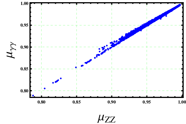
In this case, it is clear that the signal strength μγ​γ\mu_{\gamma\gamma} is also close to the SM expectation and can be still consistent with both ATLAS and CMS experimental results. In Fig. 4, we show the signal strength as a function of tan⁡β\tan\beta, where other parameters are scanned in the above-mentioned regions. For completeness, we also present the correlation between μγ​γ\mu_{\gamma\gamma} and μZ​Z\mu_{ZZ}, which equals μW​W\mu_{WW} in our model. It is remarkable that all signal strengths of Higgs decay channels in the ALRM are slightly less than the SM results.

Refer to caption
Refer to caption
Figure 4: (Left panel) The signal strength μγ​γ\mu_{\gamma\gamma} as a function of tan⁡β\tan\beta and the parameters λ3,α1,α2\lambda_{3},~\alpha_{1},~\alpha_{2} and MH1,2±M_{H^{\pm}_{1,2}}. (Right panel) Correlation between μγ​γ\mu_{\gamma\gamma} and μZ​Z\mu_{ZZ} in the ALRM.

V Signatures at the LHC

In this section we study the interesting signatures of the exotic quark d′d^{\prime} associated with our ALRM at the LHC. In particular, we will analyze and compute the cross section for the production of this heavy quark and its subsequent decays into jets, leptons and missing energy. The Lagrangian of d′d^{\prime} interactions with the SM quarks can be derived from (2) as

ℒYd′\displaystyle\mathcal{L}_{\text{Y}}^{d^{\prime}} =\displaystyle= −u¯​(cos⁡ζ​Yq​PR+sin⁡ζ​YRq​PL)​H2+​VCKM′​d′+h.c.,\displaystyle-\overline{u}~\left(\cos\zeta Y^{q}P_{R}+\sin\zeta Y^{q}_{R}P_{L}\right)~H_{2}^{+}V^{\prime}_{\text{CKM}}~d^{\prime}+\text{h.c.}~, (70)

where VCKM′V^{\prime}_{\text{CKM}} is the right-handed quark mixing matrix. In addition, the kinetic Lagrangian of d′d^{\prime} leads to the following interactions with the gauge bosons

ℒgauged′\displaystyle\mathcal{L}_{\text{gauge}}^{d^{\prime}} =\displaystyle= −i​gs2​d¯′​γμ​λa​Gμa​d′−i​g2​u¯​PR​γμ​W′μ+​VCKM′​d′−i​g2​d¯′​γμ​PR​W′μ−​V′CKM†​u\displaystyle-\frac{ig_{s}}{2}\overline{d}^{\prime}\gamma^{\mu}\lambda_{a}G_{\mu}^{a}d^{\prime}-\frac{ig}{\sqrt{2}}\overline{u}P_{R}\gamma^{\mu}{W^{\prime}}_{\mu}^{+}V^{\prime}_{\text{CKM}}d^{\prime}-\frac{ig}{\sqrt{2}}\overline{d}^{\prime}\gamma^{\mu}P_{R}{W^{\prime}}_{\mu}^{-}{V^{\prime}}_{\text{CKM}}^{\dagger}u (71)
+i3ed¯′γμ[Aμ+(P^sinϑ−12tanθwcosϑ)Zμ+(P^cosϑ+12tanθwsinϑ)Zμ′]d′,\displaystyle+\frac{i}{3}e\overline{d}^{\prime}\gamma^{\mu}\left[A_{\mu}+\left(\hat{P}\sin\vartheta-\frac{1}{2}\tan\theta_{w}\cos\vartheta\right)Z_{\mu}+\left(\hat{P}\cos\vartheta+\frac{1}{2}\tan\theta_{w}\sin\vartheta\right)Z^{\prime}_{\mu}\right]d^{\prime},

where

P^=3​cos⁡2​θw−sin2⁡θw6sinθwcosθwcos⁡2​θw​PR+sin⁡θwcosθwcos⁡2​θw​PL,\hat{P}=\frac{3\cos 2\theta_{w}-\sin^{2}\theta_{w}}{6\sin\theta_{w}\cos\theta_{w}\sqrt{\cos 2\theta_{w}}}P_{R}+\frac{\sin\theta_{w}}{\cos\theta_{w}\sqrt{\cos 2\theta_{w}}}P_{L}, (72)

where λa\lambda_{a}’s, a=1,…,8a=1,...,8, are the Gell−-Mann matrices and ϑ\vartheta is given in (15). Accordingly, in this case the pair production of d′d^{\prime} at the LHC is dominated by the following channel: g​g→d′​d′¯gg\rightarrow d^{\prime}\bar{d^{\prime}}. Considering all contributions from s,t, and u-channels, the squared amplitude of this process is given by

|ℳ⁡(g​g→d′​d′¯)|2\displaystyle\Big|{\cal M}(gg\rightarrow d^{\prime}\bar{d^{\prime}})\Big|^{2} =\displaystyle= gs424​s^2​(9​md′4−9​md′2​(s^+2​t^)+4​s^2+9​s^​t^+9​t^2)(md′2−t^)2\displaystyle\frac{g_{s}^{4}}{24\hat{s}^{2}}\frac{\left(9m_{d^{\prime}}^{4}-9m_{d^{\prime}}^{2}(\hat{s}+2\hat{t})+4\hat{s}^{2}+9\hat{s}\hat{t}+9\hat{t}^{2}\right)}{\left(m_{d^{\prime}}^{2}-\hat{t}\right)^{2}} (73)
×\displaystyle\times [md′2​(s^3+2​s^2​t^+8​s^​t^2+8​t^3)+t^​(s^+t^)​(s^2+2​s^​t^+2​t^2)(−md′2+s^+t^)2\displaystyle\Big[\frac{m_{d^{\prime}}^{2}\left(\hat{s}^{3}+2\hat{s}^{2}\hat{t}+8\hat{s}\hat{t}^{2}+8\hat{t}^{3}\right)+\hat{t}(\hat{s}+\hat{t})\left(\hat{s}^{2}+2\hat{s}\hat{t}+2\hat{t}^{2}\right)}{\left(-m_{d^{\prime}}^{2}+\hat{s}+\hat{t}\right)^{2}}
−\displaystyle- 2​md′8−8​md′6​t^+md′4​(3​s^2+4​s^​t^+12​t^2)(−md′2+s^+t^)2].\displaystyle\frac{2m_{d^{\prime}}^{8}-8m_{d^{\prime}}^{6}\hat{t}+m_{d^{\prime}}^{4}\left(3\hat{s}^{2}+4\hat{s}\hat{t}+12\hat{t}^{2}\right)}{\left(-m_{d^{\prime}}^{2}+\hat{s}+\hat{t}\right)^{2}}\Big].~~~~~

In addition the squared amplitude of the pair production of d′d^{\prime} through the channel q​q¯→γ/g→d′​d′¯q\bar{q}\to\gamma/g\to d^{\prime}\bar{d^{\prime}} is given by

|ℳ⁡(q​q¯→γ/g→d′​d¯′)|2\displaystyle\left|{\cal M}\left(q\bar{q}\rightarrow\gamma/g\rightarrow d^{\prime}\bar{d}^{\prime}\right)\right|^{2} =\displaystyle= 4​(2​g4+9​gs4)81​s^2​(2​s^​t^−4​(mq2+md′2)​t^+2​(mq2+md′2)2+2​t^2+s^2),\displaystyle\frac{4\left(2g^{4}+9g_{s}^{4}\right)}{81\hat{s}^{2}}\left(2\hat{s}\hat{t}-4\left(m_{q}^{2}+m_{d^{\prime}}^{2}\right)\hat{t}+2\left(m_{q}^{2}+m_{d^{\prime}}^{2}\right)^{2}+2\hat{t}^{2}+\hat{s}^{2}\right), (74)

where s^,t^\hat{s},\hat{t} are the partonic Mandelstam variables. The differential cross section is given by

d​σ^d​cos⁡θ=B16​π​s^2​|ℳ|2,\frac{d\hat{\sigma}}{d\cos\theta}=\frac{B}{16\pi\hat{s}^{2}}|{\cal M}|^{2}, (75)

where B=1−(4​md′2/s^)B=\sqrt{1-\left(4m_{d^{\prime}}^{2}/\hat{s}\right)}. The cross section of p​p→d′​d′pp\to d^{\prime}d^{\prime} is given by

d​σd​cos⁡θ=∑i,j∫x01d​x​fi​(x)​fj​(4​md′2s​x)​d​σ^d​cos⁡θ,\frac{d\sigma}{d\cos\theta}=\sum_{i,j}~\int_{x_{0}}^{1}dxf_{i}(x)f_{j}\Big(\frac{4m_{d^{\prime}}^{2}}{sx}\Big)~\frac{d\hat{\sigma}}{d\cos\theta}, (76)

where i,ji,j refer to the partons. The partons energy fractions are given by x1​x2=s^/s,x_{1}x_{2}=\hat{s}/s, so that the minimum parton energy fraction to produce the d′​d′d^{\prime}d^{\prime} pair is x0=2​md′/sx_{0}=2m_{d^{\prime}}/\sqrt{s}. Also, t^=−12​s^​(1−B​cos⁡θ)+Md′2\hat{t}=-\frac{1}{2}\hat{s}\left(1-B\cos\theta\right)+M^{2}_{d^{\prime}}. Therefore, one finds that the production cross section is given by

d​σ^d​t^=18​π​s^3​|ℳ|2.\frac{d\hat{\sigma}}{d\hat{t}}=\frac{1}{8\pi\hat{s}^{3}}\left|{\cal M}\right|^{2}. (77)

In Fig. 5, we display the differential cross section of the d′d^{\prime} pair production at the LHC with s=14\sqrt{s}=14 TeV as a function of the invariant mass Md′​d′M_{d^{\prime}d^{\prime}} for two choices of md′m_{d^{\prime}}, namely, md′=300m_{d^{\prime}}=300 and 500500 GeV.

Refer to caption
Refer to caption
Figure 5: Differential production cross section of exotic quark d′d^{\prime} as a function of the invariant mass Md′​d′M_{d^{\prime}d^{\prime}}. In the left panel, md′=300m_{d^{\prime}}=300 GeV, and in the right panel, md′=500m_{d^{\prime}}=500 GeV.

As can be seen from this figure, the typical value of the d′d^{\prime} production cross section is of 𝒪⁡(1){\cal O}(1) fb, which was quite accessible at the LHC during its second run. The dominant decay channel of the produced d′d^{\prime} quark is given by d′→H2+​ud^{\prime}\to H_{2}^{+}u, as indicated in (70). One can show that the corresponding decay rate is given by

Γ⁡(d′→u​H2+)=|VCKM′|216​π​ℏ​(|Yq|2​cos2⁡ζ+|YRq|2​sin2⁡ζ)​md′​(1−MH2+2md′2)2.\Gamma\left(d^{\prime}\rightarrow uH_{2}^{+}\right)=\frac{|V^{\prime}_{\text{CKM}}|^{2}}{16\pi\hbar}\left(|Y^{q}|^{2}\cos^{2}\zeta+|Y^{q}_{R}|^{2}\sin^{2}\zeta\right)m_{d^{\prime}}\left(1-\frac{M_{H_{2}^{+}}^{2}}{m_{d^{\prime}}^{2}}\right)^{2}. (78)

Here, we assumed that mu≪md′m_{u}\ll m_{d^{\prime}}. On the other hand, the charged Higgs boson H2+H_{2}^{+} decays into a lepton and scotino through the interactions

ℒYH2+=n¯​H2+​UMNS′​(cos⁡ζ​Yℓ​PL+sin⁡ζ​YRℓ​PR)​e+h.c..\mathcal{L}_{\text{Y}}^{H_{2}^{+}}=\overline{n}~H_{2}^{+}~U^{\prime}_{\text{MNS}}\left(\cos\zeta Y^{\ell}P_{L}+\sin\zeta Y^{\ell}_{R}P_{R}\right)~e+\text{h.c.}~. (79)

Thus, the decay rate of H2−→e−​nH_{2}^{-}\to e^{-}n, for me=0m_{e}=0, is given by

Γ⁡(H2−→e−​n)=|UMNS′|216​π​ℏ​(|Yℓ|2​cos2⁡ζ+|YRℓ|2​sin2⁡ζ)​MH2+​(1−mn2MH2+2)2.\Gamma\left(H_{2}^{-}\rightarrow e^{-}n\right)=\frac{|U^{\prime}_{\text{MNS}}|^{2}}{16\pi\hbar}\left(|Y^{\ell}|^{2}\cos^{2}\zeta+|Y^{\ell}_{R}|^{2}\sin^{2}\zeta\right)M_{H_{2}^{+}}\left(1-\frac{m_{n}^{2}}{M_{H_{2}^{+}}^{2}}\right)^{2}. (80)
Refer to caption
Figure 6: The exotic quark, d′d^{\prime}, creation and decay.

In Fig. 6, we show the total cross section of this process with an opposite-sign dilepton, which is the most striking signature for this exotic quark at the LHC. This cross section can be approximately written as

σ⁡(g​g→g→d′​d¯′→l∓​l±+ETmiss+jets)\displaystyle\sigma\left(gg\rightarrow g\rightarrow d^{\prime}\overline{d}^{\prime}\rightarrow l^{\mp}l^{\pm}+E_{T}^{\text{miss}}+\text{jets}\right) ≃\displaystyle\simeq σ⁡(g​g→g→d′​d¯′)\displaystyle\sigma\left(gg\rightarrow g\rightarrow d^{\prime}\overline{d}^{\prime}\right) (81)
×\displaystyle\times BR​(d′→H2++jets)2​BR​(H2∓→l∓+ETmiss)2.\displaystyle\text{BR}\left(d^{\prime}\rightarrow H_{2}^{+}+\text{jets}\right)^{2}\text{BR}\left(H_{2}^{\mp}\rightarrow l^{\mp}+E_{T}^{\text{miss}}\right)^{2}.

Since the dominant decay channel of d′d^{\prime} is d′→u​H2−d^{\prime}\rightarrow uH_{2}^{-} and the charged Higgs decays mainly to l±+nl^{\pm}+n, one finds BR​(d′→u​H2−)≃1\text{BR}\left(d^{\prime}\rightarrow uH_{2}^{-}\right)\simeq 1 and BR​(H2±→l±​n)≃1\text{BR}\left(H_{2}^{\pm}\rightarrow l^{\pm}n\right)\simeq 1. Therefore, σ⁡(g​g→g→d′​d¯′→l∓​l±+ETmiss+jets)≃σ⁡(g​g→g→d′​d¯′)≃𝒪⁡(1)\sigma\left(gg\rightarrow g\rightarrow d^{\prime}\overline{d}^{\prime}\rightarrow l^{\mp}l^{\pm}+E_{T}^{\text{miss}}+\text{jets}\right)\simeq\sigma\left(gg\rightarrow g\rightarrow d^{\prime}\overline{d}^{\prime}\right)\simeq{\cal O}(1) fb, which can be accessible at the LHC with s≃14\sqrt{s}\simeq 14 TeV. In Fig. 7, we show the reconstructed invariant mass of the extra quark d′d^{\prime}, which decays into l+n⁡(scotino)+j​e​tl+n({\rm scotino})+jet, with all possible background. In this figure, we have not imposed any cut yet. Therefore, the background is clearly dominated the signal. Here, we assume md′=300m_{d^{\prime}}=300 GeV, the charged Higgs mass is of order 200200 GeV, and the LHC integrated luminosity is of order 200200 fb-1.

Refer to caption
Figure 7: The reconstructed invariant mass of extra quark, d′d^{\prime}, which decays to l+j​e​t+missing​energyl+jet+{\rm missing~energy} and its background for md′=300m_{d^{\prime}}=300 GeV. No cut has been imposed yet.

In Fig. 8 (left panel), we plot the number of reconstructed events per bin of the invariant mass of d′d^{\prime} of the above process for signal and SM background at E̸T​cut>200\not{E}_{T}~{\rm cut}>200 GeV, where E̸T\not{E}_{T} is the missing transverse energy, E̸T=||∑visible particlesp→T||\not{E}_{T}=\left|\left|\sum_{\text{visible particles}}\vec{p}_{T}\right|\right|, with md′=300m_{d^{\prime}}=300 GeV and s=14\sqrt{s}=14 TeV. This figure shows that it is possible to extract a good significance for the extra-quark signal in this channel. In addition, we also impose a cut, HT<200H_{T}<200 GeV, where HTH_{T} is the total transverse hadronic energy: HT=∑hadronic particles||p→T||H_{T}=\sum_{\text{hadronic particles}}\left|\left|\vec{p}_{T}\right|\right|. It is remarkable that with HTH_{T} cuts the signal can be much larger than the background. We have used Feynrules [36] to generate the model files and Calchep [37] and MadEvent5 [38, 39] to calculate the numerical values of the cross sections and number of events, respectively.

Refer to caption
Refer to caption
Figure 8: The reconstructed invariant mass of the extra quark, d′d^{\prime}, which decays to l+j​e​t+missing​energyl+jet+{\rm missing~energy} for md′=300m_{d^{\prime}}=300 GeV, with E̸T>200\not{E}_{T}>200 GeV cut (left panel) and HT<200H_{T}<200 GeV cut (right panel).

Finally, we provide in Table 2 some details for the used cuts on PTP_{T} and HTH_{T} on the signal and background for the process p​p→d′​d′→(l−​l+)+(u​u¯)+(n​n)pp\to d^{\prime}d^{\prime}\to(l^{-}l^{+})+(u\bar{u})+(nn). As can be seen from the results in this table, the signal of this process can be much larger than the background if one imposes the proper HTH_{T} cuts. It is worth mentioning that the Higgs sector of our model is very similar to the two Higgs doublets in the minimal supersymmetric standard model, where one Higgs doublet couples to up quarks and the second couples to down quarks. Therefore, it does not lead to any flavor-changing neutral current problem, and a light charged Higgs is phenomenologically acceptable. The number of events of exotic quark d′d^{\prime} at the LHC may slightly changed if a heavier charged Higgs is considered, but with keeping mH+<md′m_{H^{+}}<m_{d^{\prime}}, to ensure that BR​(d​’→H++j​e​t​s)∼1\text{BR}(d’\rightarrow H^{+}+jets)\sim 1.

Cuts (GeV) Signal (S) Background (B) S vs B
Initial (no cut) 463999 9309732 ±\pm 21646 0.049840 ±\pm 0.000116
Cut 1 (E̸T>200\not{E}_{T}>200) 72291 ±\pm 247 33523 ±\pm 198 2.1564 ±\pm 0.0148
Cut 2 (HT<200H_{T}<200) 47977 ±\pm 207 1942.7 ±\pm 44.3 24.696 ±\pm 0.573
Table 2: Signal vs background for the process p​p→d′​d′→(l−​l+)+(u​u¯)+(n​n)pp\to d^{\prime}d^{\prime}\to(l^{-}l^{+})+(u\bar{u})+(nn) with/without cuts.

VI Conclusions

In this paper, we have analyzed some phenomenological aspects of the alternative left-right model, motivated by the superstring-inspired E6E_{6} model. We provided a detailed analysis for the symmetry breaking and Higgs sector of this model, which consists of four neutral C​PCP-even Higgs, two C​PCP-odd Higgs and two charged Higgs bosons. We emphasized that three neutral C​PCP-even Higgs and two C​PCP-odd Higgs in addition to two charged Higgs can be light, of 𝒪⁡(100){\cal O}(100) GeV. We also found that the contributions of charged Higgs bosons and the extra exotic quark d′d^{\prime} to H→γ​γH\to\gamma\gamma are quite negligible. Therefore, our model predicts signal strengths of Higgs decay, in particular, of H→γ​γH\to\gamma\gamma and H→W+​W−H\to W^{+}W^{-} that coincide with the SM expectations.

Finally, we studied the striking signatures of the exotic down-type quark at the LHC. In particular, we computed the cross section of d′d^{\prime}-pair production . We showed that the typical value of this cross section is of 𝒪⁡(1){\cal O}(1) fb, which is quite accessible at the LHC. The decay of d′d^{\prime} into a jet, lepton, and missing energy provides an important signature for this class of models at the LHC.

Acknowledgments

This work is partially supported by the ICTP Grant No. AC-80. M. Ashry would like to thank W. Abdallah, A. Elsayed, A. Hammad and A. Moursy for fruitful discussions.

Appendix

To study the boundedness from below, and hence the stability, of the potential (20) we use the following theorem [24, 25] to ensure that the matrix of the quartic terms, which are dominant at higher values of the fields, is copositive:

Theorem 1 (Copositivity Criteria)

Let a∈ℝ,b∈ℝn−1a\in\mathbb{R},\ b\in\mathbb{R}^{n-1} and C∈ℝ(n−1)×(n−1)C\in\mathbb{R}^{(n-1)\times(n-1)}. The symmetric matrix M∈ℝn×nM\in\mathbb{R}^{n\times n}

M=(abTbC),\displaystyle M=\left(\begin{array}[]{cc}a&b^{T}\\ b&C\end{array}\right),

is copositive if and only if

  1. 1.

    a≥0,Ca\geq 0,\ C is copositive,

  2. 2.

    for any nonzero vector y∈ℝ(n−1)y\in\mathbb{R}^{(n-1)}, with y≥0y\geq 0, if bT​y≤0b^{T}y\leq 0, it follows that yT​(a​C−b​bT)​y≥0.y^{T}\left(aC-bb^{T}\right)y\geq 0.

The quartic terms of the potential (20) can be written as

V4​F​(ϕ1,20,+,χL,R0,+){}^{4F}V\left(\phi_{1,2}^{0,+},\chi_{L,R}^{0,+}\right) =\displaystyle= λ1​(|ϕ10|4+|ϕ1+|4+|ϕ20|4+|ϕ2+|4)+λ3​(|χL0|4+|χL+|4+|χR0|4+|χR+|4)\displaystyle\lambda_{1}\left(\left|\phi_{1}^{0}\right|^{4}+\left|\phi_{1}^{+}\right|^{4}+\left|\phi_{2}^{0}\right|^{4}+\left|\phi_{2}^{+}\right|^{4}\right)+\lambda_{3}\left(\left|\chi_{L}^{0}\right|^{4}+\left|\chi_{L}^{+}\right|^{4}+\left|\chi_{R}^{0}\right|^{4}+\left|\chi_{R}^{+}\right|^{4}\right) (85)
+\displaystyle+ 2​|ϕ10|2​[λ1​(|ϕ1+|2+|ϕ2+|2)+λ12​|ϕ20|2+α13​(|χL0|2+|χR0|2)+α12​(|χL+|2+|χR+|2)]\displaystyle 2\left|\phi_{1}^{0}\right|^{2}\left[\lambda_{1}\left(\left|\phi_{1}^{+}\right|^{2}+\left|\phi_{2}^{+}\right|^{2}\right)+\lambda_{12}\left|\phi_{2}^{0}\right|^{2}+\alpha_{13}\left(\left|\chi_{L}^{0}\right|^{2}+\left|\chi_{R}^{0}\right|^{2}\right)+\alpha_{12}\left(\left|\chi_{L}^{+}\right|^{2}+\left|\chi_{R}^{+}\right|^{2}\right)\right]
+\displaystyle+ 2​|ϕ1+|2​[λ1​|ϕ20|2+λ12​|ϕ2+|2+α13​(|χL0|2+|χR+|2)+α12​(|χL+|2+|χR0|2)]\displaystyle 2\left|\phi_{1}^{+}\right|^{2}\left[\lambda_{1}\left|\phi_{2}^{0}\right|^{2}+\lambda_{12}\left|\phi_{2}^{+}\right|^{2}+\alpha_{13}\left(\left|\chi_{L}^{0}\right|^{2}+\left|\chi_{R}^{+}\right|^{2}\right)+\alpha_{12}\left(\left|\chi_{L}^{+}\right|^{2}+\left|\chi_{R}^{0}\right|^{2}\right)\right]
+\displaystyle+ 2​|ϕ20|2​[λ1​|ϕ2+|2+α12​(|χL0|2+|χR0|2)+α13​(|χL+|2+|χR+|2)]\displaystyle 2\left|\phi_{2}^{0}\right|^{2}\left[\lambda_{1}\left|\phi_{2}^{+}\right|^{2}+\alpha_{12}\left(\left|\chi_{L}^{0}\right|^{2}+\left|\chi_{R}^{0}\right|^{2}\right)+\alpha_{13}\left(\left|\chi_{L}^{+}\right|^{2}+\left|\chi_{R}^{+}\right|^{2}\right)\right]
+\displaystyle+ 2​|ϕ2+|2​[α12​(|χL0|2+|χR+|2)+α13​(|χL+|2+|χR0|2)]\displaystyle 2\left|\phi_{2}^{+}\right|^{2}\left[\alpha_{12}\left(\left|\chi_{L}^{0}\right|^{2}+\left|\chi_{R}^{+}\right|^{2}\right)+\alpha_{13}\left(\left|\chi_{L}^{+}\right|^{2}+\left|\chi_{R}^{0}\right|^{2}\right)\right]
+\displaystyle+ 2​|χL0|2​(λ3​|χL+|2+λ4​|χR0|2+λ4​|χR+|2)+2​|χL+|2​(λ4​|χR0|2+λ4​|χR+|2)\displaystyle 2\left|\chi_{L}^{0}\right|^{2}\left(\lambda_{3}\left|\chi_{L}^{+}\right|^{2}+\lambda_{4}\left|\chi_{R}^{0}\right|^{2}+\lambda_{4}\left|\chi_{R}^{+}\right|^{2}\right)+2\left|\chi_{L}^{+}\right|^{2}\left(\lambda_{4}\left|\chi_{R}^{0}\right|^{2}+\lambda_{4}\left|\chi_{R}^{+}\right|^{2}\right)
+\displaystyle+ 2​λ3​|χR0|2​|χR+|2−8​λ2​R​e​[ϕ10​ϕ1−​ϕ20​ϕ2+]\displaystyle 2\lambda_{3}\left|\chi_{R}^{0}\right|^{2}\left|\chi_{R}^{+}\right|^{2}-8\lambda_{2}Re\left[\phi_{1}^{0}\phi_{1}^{-}\phi_{2}^{0}\phi_{2}^{+}\right]
+\displaystyle+ 4​(α2−α3)​R​e​[(ϕ10​ϕ2++ϕ20∗​ϕ1+)​χL0​χL−+(ϕ20​ϕ2++ϕ10∗​ϕ1+)​χR0​χR−],\displaystyle 4(\alpha_{2}-\alpha_{3})Re\left[\left(\phi_{1}^{0}\phi_{2}^{+}+{\phi_{2}^{0}}^{*}\phi_{1}^{+}\right)\chi_{L}^{0}\chi_{L}^{-}+\left(\phi_{2}^{0}\phi_{2}^{+}+{\phi_{1}^{0}}^{*}\phi_{1}^{+}\right)\chi_{R}^{0}\chi_{R}^{-}\right],

where α12=α1+α2,α13=α1+α3\alpha_{12}=\alpha_{1}+\alpha_{2},\ \alpha_{13}=\alpha_{1}+\alpha_{3} and λ12=λ1+2​λ2\lambda_{12}=\lambda_{1}+2\lambda_{2}. We have

ϕ1,20,+=|ϕ1,20,+|​exp⁡[i​θ1,20,+],χL,R0,+=|χL,R0,+|​exp⁡[i​θL,R0,+].\phi_{1,2}^{0,+}=|\phi_{1,2}^{0,+}|\exp\left[i\theta_{1,2}^{0,+}\right],~~~~~\chi_{L,R}^{0,+}=|\chi_{L,R}^{0,+}|\exp\left[i\theta_{L,R}^{0,+}\right]. (86)

By the redefinitions of the fields’ components,

ϕ1+→ϕ1+​exp​[i⁡(θ10−θ1+)],ϕ20→ϕ20​exp​[i⁡(θ10−θ20)],ϕ2+→ϕ2+​exp​[−i⁡(θ10+θ2+)],\phi_{1}^{+}\to\phi_{1}^{+}\exp\left[i\left(\theta_{1}^{0}-\theta_{1}^{+}\right)\right],\phi_{2}^{0}\to\phi_{2}^{0}\exp\left[i\left(\theta_{1}^{0}-\theta_{2}^{0}\right)\right],\phi_{2}^{+}\to\phi_{2}^{+}\exp\left[-i\left(\theta_{1}^{0}+\theta_{2}^{+}\right)\right], (87)
χL,R+→χL,R+​exp⁡[i⁡(θL,R0−θL,R+)],\chi_{L,R}^{+}\to\chi_{L,R}^{+}\exp\left[i\left(\theta_{L,R}^{0}-\theta_{L,R}^{+}\right)\right], (88)

we can write

V4​F​(ϕ1,20,+,χL,R0,+){}^{4F}V\left(\phi_{1,2}^{0,+},\chi_{L,R}^{0,+}\right) =\displaystyle= XT​V4​F​X−8​λ2​|ϕ10|​|ϕ1−​‖ϕ20‖​ϕ2+|\displaystyle X^{T}~{}^{4F}V~X-8\lambda_{2}|\phi_{1}^{0}||\phi_{1}^{-}||\phi_{2}^{0}||\phi_{2}^{+}| (89)
+\displaystyle+ 4​(α2−α3)​[(|ϕ10|​|ϕ2+|+|ϕ20|​|ϕ1+|)​|χL0​‖χL+​|+(|ϕ20|​|ϕ2+​|+|ϕ10||​ϕ1+|)|​χR0‖​χR+|],\displaystyle 4(\alpha_{2}-\alpha_{3})\left[\left(|\phi_{1}^{0}||\phi_{2}^{+}|+|\phi_{2}^{0}||\phi_{1}^{+}|\right)|\chi_{L}^{0}||\chi_{L}^{+}|+\left(|\phi_{2}^{0}||\phi_{2}^{+}|+|\phi_{1}^{0}||\phi_{1}^{+}|\right)|\chi_{R}^{0}||\chi_{R}^{+}|\right],

where

XT\displaystyle X^{T} =\displaystyle= (|ϕ10|2|ϕ1+|2|ϕ20|2|ϕ2+|2|χL0|2|χL+|2|χR0|2|χR+|2),\displaystyle\left(\begin{array}[]{cccccccc}\left|\phi_{1}^{0}\right|^{2}&\left|\phi_{1}^{+}\right|^{2}&\left|\phi_{2}^{0}\right|^{2}&\left|\phi_{2}^{+}\right|^{2}&\left|\chi_{L}^{0}\right|^{2}&\left|\chi_{L}^{+}\right|^{2}&\left|\chi_{R}^{0}\right|^{2}&\left|\chi_{R}^{+}\right|^{2}\end{array}\right),
V4​F{}^{4F}V =\displaystyle= (λ1λ1λ12λ1α13α12α13α12λ1λ1λ1λ12α13α12α12α13λ12λ1λ1λ1α12α13α12α13λ1λ12λ1λ1α12α13α13α12α13α13α12α12λ3λ3λ4λ4α12α12α13α13λ3λ3λ4λ4α13α12α12α13λ4λ4λ3λ3α12α13α13α12λ4λ4λ3λ3).\displaystyle\left(\begin{array}[]{cccccccc}\lambda_{1}&~~\lambda_{1}&~~~\lambda_{12}&~~\lambda_{1}&~~\alpha_{13}&~~~\alpha_{12}&~~~\alpha_{13}&~~~\alpha_{12}\\ \lambda_{1}&~~\lambda_{1}&~~~\lambda_{1}&~~\lambda_{12}&~~\alpha_{13}&~~~\alpha_{12}&~~~\alpha_{12}&~~~\alpha_{13}\\ \lambda_{12}&~~\lambda_{1}&~~~\lambda_{1}&~~\lambda_{1}&~~\alpha_{12}&~~~\alpha_{13}&~~~\alpha_{12}&~~~\alpha_{13}\\ \lambda_{1}&~~\lambda_{12}&~~~\lambda_{1}&~~\lambda_{1}&~~\alpha_{12}&~~~\alpha_{13}&~~~\alpha_{13}&~~~\alpha_{12}\\ \alpha_{13}&~~\alpha_{13}&~~~\alpha_{12}&~~\alpha_{12}&~~~\lambda_{3}&~~~\lambda_{3}&~~~\lambda_{4}&~~~\lambda_{4}\\ \alpha_{12}&~~\alpha_{12}&~~~\alpha_{13}&~~\alpha_{13}&~~~\lambda_{3}&~~~\lambda_{3}&~~~\lambda_{4}&~~~\lambda_{4}\\ \alpha_{13}&~~\alpha_{12}&~~~\alpha_{12}&~~\alpha_{13}&~~~\lambda_{4}&~~~\lambda_{4}&~~~\lambda_{3}&~~~\lambda_{3}\\ \alpha_{12}&~~\alpha_{13}&~~~\alpha_{13}&~~\alpha_{12}&~~~\lambda_{4}&~~~\lambda_{4}&~~~\lambda_{3}&~~~\lambda_{3}\end{array}\right).

For the potential (85) to be bounded from below, it must happen that the matrix V4​F{}^{4F}V is copositive and λ2≤0\lambda_{2}\leq 0 and α2−α3≥0\alpha_{2}-\alpha_{3}\geq 0. The pseudoscalar Higgs mass (39) implies that μ3<0\mu_{3}<0. With the minimization condition (22), both imply that λ4>λ3\lambda_{4}>\lambda_{3}. The copositivity implies that the diagonal elements λ1,λ3≥0\lambda_{1},\lambda_{3}\geq 0. Accordingly, λ4>λ3≥0\lambda_{4}>\lambda_{3}\geq 0. It is remarkable that the copositivity of the matrix V4​F{}^{4F}V significantly depends on the signs of the parameters α12,α13\alpha_{12},\ \alpha_{13}, and λ12\lambda_{12}. Here we present the cases depending on these signs:

  1. 1.

    α12≥0,α13≥0\alpha_{12}\geq 0,\ \alpha_{13}\geq 0, and λ12≥0\lambda_{12}\geq 0: In this case, the matrix V4​F{}^{4F}V is copositive, and the potential is bounded from below.

  2. 2.

    α12≥0,α13≥0\alpha_{12}\geq 0,\ \alpha_{13}\geq 0, and λ12≤0\lambda_{12}\leq 0: The copositivity conditions are

    λ1+λ2≥0,λ12+8​λ1​λ2+4​λ22≤0.\lambda_{1}+\lambda_{2}\geq 0,~\lambda_{1}^{2}+8\lambda_{1}\lambda_{2}+4\lambda_{2}^{2}\leq 0. (101)

    We deduce these conditions in detail considering the case assumptions and using Theorem 1. To make the 8×88\times 8 matrix V4​F{}^{4F}V be copositive, we shall make that first with the 7×77\times 7 matrix, CC, arising from the matrix V4​F{}^{4F}V by eliminating the first row and the first column. In our case, it is sufficient to stop at this level, since the 6×66\times 6 matrix, C1C_{1}, arising from the matrix V4​F{}^{4F}V by eliminating the first two rows and the first two columns is already copositive; being a matrix of nonnegative elements. Now,

    V4​F{}^{4F}V =\displaystyle= (λ1bTbC),bT=(λ1λ12λ1α13α12α13α12),\displaystyle\left(\begin{array}[]{cc}\lambda_{1}&b^{T}\\ b&C\end{array}\right),~~~~~b^{T}=\left(\begin{array}[]{ccccccc}\lambda_{1}&\lambda_{12}&\lambda_{1}&\alpha_{13}&\alpha_{12}&\alpha_{13}&\alpha_{12}\end{array}\right),
    C\displaystyle C =\displaystyle= (λ1b1Tb1C1),b1T=(λ1λ12α13α12α12α13).\displaystyle\left(\begin{array}[]{cc}\lambda_{1}&b_{1}^{T}\\ b_{1}&C_{1}\end{array}\right),~~~~~b_{1}^{T}=\left(\begin{array}[]{cccccc}\lambda_{1}&\lambda_{12}&\alpha_{13}&\alpha_{12}&\alpha_{12}&\alpha_{13}\end{array}\right).

    Let y1T=(x1x2x3x4x5x6)y_{1}^{T}=\left(\begin{array}[]{cccccc}x_{1}&x_{2}&x_{3}&x_{4}&x_{5}&x_{6}\end{array}\right) be a vector that satisfies Theorem 1 requests, i.e., a nonzero and a nonnegative vector. Taking x2≠0,x1,3,…,6=0x_{2}\neq 0,\ x_{1,3,...,6}=0, makes the linear form b1T​y1=λ12​x2≤0b_{1}^{T}y_{1}=\lambda_{12}x_{2}\leq 0 and its corresponding quadratic form

    y1T​(λ1​C1−b1​b1T)​y1=−4​λ2​(λ1+λ2)​x22.y_{1}^{T}\left(\lambda_{1}C_{1}-b_{1}b_{1}^{T}\right)y_{1}=-4\lambda_{2}(\lambda_{1}+\lambda_{2})x_{2}^{2}.

    Since we have λ2≤0\lambda_{2}\leq 0, we impose the condition

    λ1+λ2≥0\lambda_{1}+\lambda_{2}\geq 0 (110)

    to make the quadratic form y1T​(λ1​C1−b1​b1T)​y≥0y_{1}^{T}\left(\lambda_{1}C_{1}-b_{1}b_{1}^{T}\right)y\geq 0 and hence as a necessary condition for the copositivity.

    Let us assume that xi≠0,i=1,…,6x_{i}\neq 0,\ i=1,...,6. Then, the linear form

    b1T​y1≤0⟷x2≥x2min=1−λ12​(λ1​x1+α13​x3+α12​x4+α12​x5+α13​x6).b_{1}^{T}y_{1}\leq 0\longleftrightarrow x_{2}\geq x_{2}^{\text{min}}=\frac{1}{-\lambda_{12}}(\lambda_{1}x_{1}+\alpha_{13}x_{3}+\alpha_{12}x_{4}+\alpha_{12}x_{5}+\alpha_{13}x_{6}).

    The copositivity condition (110) makes the corresponding quadratic form be increasing in x2x_{2} (for any fixed values of the other xix_{i}’s), and hence we deduce that

    y1T​(λ1​C1−b1​b1T)​y1≥y1T​(λ1​C1−b1​b1T)​y1|x2=x2min\displaystyle y_{1}^{T}\left(\lambda_{1}C_{1}-b_{1}b_{1}^{T}\right)y_{1}\geq y_{1}^{T}\left(\lambda_{1}C_{1}-b_{1}b_{1}^{T}\right)y_{1}\Big|_{x_{2}=x_{2}^{\text{min}}}
    =λ1λ122[4λ1λ22x12−2λ2(α13λ1−α12λ12)x1x3−2λ2(α12λ1−α13λ12)x1x4\displaystyle=\frac{\lambda_{1}}{\lambda_{12}^{2}}\Big[4\lambda_{1}\lambda_{2}^{2}x_{1}^{2}-2\lambda_{2}\left(\alpha_{13}\lambda_{1}-\alpha_{12}\lambda_{12}\right)x_{1}x_{3}-2\lambda_{2}\left(\alpha_{12}\lambda_{1}-\alpha_{13}\lambda_{12}\right)x_{1}x_{4}
    +2​x1​((α12​x5+α13​x6)​(λ12+2​λ1​λ2+4​λ22)−2​(α13​x5+α12​x6)​λ1​λ12)\displaystyle+2x_{1}\left((\alpha_{12}x_{5}+\alpha_{13}x_{6})(\lambda_{1}^{2}+2\lambda_{1}\lambda_{2}+4\lambda_{2}^{2})-2(\alpha_{13}x_{5}+\alpha_{12}x_{6})\lambda_{1}\lambda_{12}\right)
    +x3​((α132​λ1−2​α12​α13​λ12)​(x3+2​x6)+λ122​(λ3​x3+2​λ4​x6))\displaystyle+x_{3}\left((\alpha_{13}^{2}\lambda_{1}-2\alpha_{12}\alpha_{13}\lambda_{12})(x_{3}+2x_{6})+\lambda_{12}^{2}(\lambda_{3}x_{3}+2\lambda_{4}x_{6})\right)
    +2​x3​((α12​α13​λ1−λ12​(α122+α132))​(x4+x5)+λ122​(λ3​x4+λ4​x5))\displaystyle+2x_{3}\left((\alpha_{12}\alpha_{13}\lambda_{1}-\lambda_{12}(\alpha_{12}^{2}+\alpha_{13}^{2}))(x_{4}+x_{5})+\lambda_{12}^{2}(\lambda_{3}x_{4}+\lambda_{4}x_{5})\right)
    +x4​((α122​λ1−2​α12​α13​λ12)​(x4+2​x5)+λ122​(λ3​x4+2​λ4​x5))\displaystyle+x_{4}\left((\alpha_{12}^{2}\lambda_{1}-2\alpha_{12}\alpha_{13}\lambda_{12})(x_{4}+2x_{5})+\lambda_{12}^{2}(\lambda_{3}x_{4}+2\lambda_{4}x_{5})\right)
    +2​x6​((α12​α13​λ1−λ12​(α122+α132))​(x4+x5)+λ122​(λ4​x4+λ3​x5))\displaystyle+2x_{6}\left((\alpha_{12}\alpha_{13}\lambda_{1}-\lambda_{12}(\alpha_{12}^{2}+\alpha_{13}^{2}))(x_{4}+x_{5})+\lambda_{12}^{2}(\lambda_{4}x_{4}+\lambda_{3}x_{5})\right)
    +(α122λ1−2α12α13λ12+λ122λ3)x52+(α132λ1−2α12α13λ12+λ122λ3)x62].\displaystyle+\left(\alpha_{12}^{2}\lambda_{1}-2\alpha_{12}\alpha_{13}\lambda_{12}+\lambda_{12}^{2}\lambda_{3}\right)x_{5}^{2}+\left(\alpha_{13}^{2}\lambda_{1}-2\alpha_{12}\alpha_{13}\lambda_{12}+\lambda_{12}^{2}\lambda_{3}\right)x_{6}^{2}\Big].~~~~~~~~ (111)

    By the case assumptions and the copositivity condition (110), the quadratic form (111) is non-negative termwise and the theorem is satisfied.

    For the copositivity of the matrix V4​F{}^{4F}V, let yT=(x1x2x3x4x5x6x7)y^{T}=\left(\begin{array}[]{ccccccc}x_{1}&x_{2}&x_{3}&x_{4}&x_{5}&x_{6}&x_{7}\end{array}\right) be a nonzero and a non-negative vector. Let x1,2,3≠0,x4,…,7=0x_{1,2,3}\neq 0,\ x_{4,...,7}=0. Then the linear form

    bT​y=λ1​(x1+x3)+λ12​x2≤0⟷x2≥x2min=λ1−λ12​(x1+x3).b^{T}y=\lambda_{1}(x_{1}+x_{3})+\lambda_{12}x_{2}\leq 0\longleftrightarrow x_{2}\geq x_{2}^{\text{min}}=\frac{\lambda_{1}}{-\lambda_{12}}(x_{1}+x_{3}).

    Condition (110) makes the corresponding quadratic form

    yT​(λ1​C−b​bT)​y=−4​λ2​(x1​(x2−x3)​λ1+x2​(x3​λ1+x2​(λ1+λ2)))y^{T}\left(\lambda_{1}C-bb^{T}\right)y=-4\lambda_{2}\left(x_{1}(x_{2}-x_{3})\lambda_{1}+x_{2}(x_{3}\lambda_{1}+x_{2}(\lambda_{1}+\lambda_{2}))\right)

    be increasing in x2x_{2} (for any fixed values of x1,3x_{1,3}), and hence we deduce that

    yT​(λ1​C−b​bT)​y\displaystyle y^{T}\left(\lambda_{1}C-bb^{T}\right)y ≥\displaystyle\geq yT​(λ1​C−b​bT)​y|x2=x2min\displaystyle y^{T}\left(\lambda_{1}C-bb^{T}\right)y\Big|_{x_{2}=x_{2}^{\text{min}}}
    =\displaystyle= 4​λ1λ122​(λ1​λ22​x12+λ2​(λ12+6​λ1​λ2+4​λ22)​x1​x3+λ1​λ22​x32)≥0\displaystyle\frac{4\lambda_{1}}{\lambda_{12}^{2}}\left(\lambda_{1}\lambda_{2}^{2}x_{1}^{2}+\lambda_{2}(\lambda_{1}^{2}+6\lambda_{1}\lambda_{2}+4\lambda_{2}^{2})x_{1}x_{3}+\lambda_{1}\lambda_{2}^{2}x_{3}^{2}\right)\geq 0
    =\displaystyle= 4​λ1λ122​X13T​M13​X13,∀x1,3,\displaystyle\frac{4\lambda_{1}}{\lambda_{12}^{2}}X_{13}^{T}M_{13}X_{13},\ \forall x_{1,3},

    where

    M13=(λ1​λ2212​λ2​(λ12+6​λ1​λ2+4​λ22)12​λ2​(λ12+6​λ1​λ2+4​λ22)λ1​λ22),X13​(x1x3).M_{13}=\left(\begin{array}[]{cc}\lambda_{1}\lambda_{2}^{2}&\frac{1}{2}\lambda_{2}(\lambda_{1}^{2}+6\lambda_{1}\lambda_{2}+4\lambda_{2}^{2})\\ \frac{1}{2}\lambda_{2}(\lambda_{1}^{2}+6\lambda_{1}\lambda_{2}+4\lambda_{2}^{2})&\lambda_{1}\lambda_{2}^{2}\end{array}\right),~~~~~X_{13}\left(\begin{array}[]{c}x_{1}\\ x_{3}\end{array}\right).

    Now, yT​(λ1​C−b​bT)​y|x2=x2min≥0y^{T}\left(\lambda_{1}C-bb^{T}\right)y\Big|_{x_{2}=x_{2}^{\text{min}}}\geq 0 is equivalent to the copositivity of the matrix M13M_{13}. Equivalently,

    λ12+8​λ1​λ2+4​λ22≤0.\lambda_{1}^{2}+8\lambda_{1}\lambda_{2}+4\lambda_{2}^{2}\leq 0. (112)

    Now, assume that xi≠0,i=1,…,7x_{i}\neq 0,\ i=1,...,7. Then, the linear form

    bT​y≤0⟷x2≥x2min=1−λ12​(λ1​x1+λ1​x3+α13​x4+α12​x5+α13​x6+α12​x7).b^{T}y\leq 0\longleftrightarrow x_{2}\geq x_{2}^{\text{min}}=\frac{1}{-\lambda_{12}}(\lambda_{1}x_{1}+\lambda_{1}x_{3}+\alpha_{13}x_{4}+\alpha_{12}x_{5}+\alpha_{13}x_{6}+\alpha_{12}x_{7}).

    As before, conditions (110, 112) make

    yT​(λ1​C−b​bT)​y\displaystyle y^{T}\left(\lambda_{1}C-bb^{T}\right)y ≥\displaystyle\geq yT​(λ1​C−b​bT)​y|x2=x2min≥0,∀x1,3,..,6.\displaystyle y^{T}\left(\lambda_{1}C-bb^{T}\right)y\Big|_{x_{2}=x_{2}^{\text{min}}}\geq 0,\ \forall x_{1,3,..,6}.

    Hence, the theorem is satisfied, and, finally, the only imposed conditions for the matrix V4​F{}^{4F}V to be copositive in this case are those in (101). The same procedure is followed to extract the copositivity conditions in the following cases:

  3. 3.

    α12≥0,α13≤0\alpha_{12}\geq 0,\ \alpha_{13}\leq 0, and λ12≥0\lambda_{12}\geq 0: The following conditions are necessary for the copositivity:

    λ1​λ3−α132≥0,α132​(λ3−λ4)≥0.\lambda_{1}\lambda_{3}-\alpha_{13}^{2}\geq 0,~\alpha_{13}^{2}(\lambda_{3}-\lambda_{4})\geq 0.

    Since λ4−λ3>0\lambda_{4}-\lambda_{3}>0, then we must have α13=0\alpha_{13}=0. Finally, in this case, the copositivity conditions are

    α12≥0,α13=0,λ12≥0.\alpha_{12}\geq 0,\ \alpha_{13}=0,\ \lambda_{12}\geq 0. (113)
  4. 4.

    α12≤0,α13≥0\alpha_{12}\leq 0,\ \alpha_{13}\geq 0, and λ12≥0\lambda_{12}\geq 0: The following conditions are necessary for the copositivity:

    λ1​λ3−α122≥0,α122​(α12−α13)2​λ12​(λ32−λ42)≥0.\lambda_{1}\lambda_{3}-\alpha_{12}^{2}\geq 0,~\alpha_{12}^{2}(\alpha_{12}-\alpha_{13})^{2}\lambda_{1}^{2}\left(\lambda_{3}^{2}-\lambda_{4}^{2}\right)\geq 0.

    Again, either α12=0,α12=α13\alpha_{12}=0,\ \alpha_{12}=\alpha_{13}, or λ1=0\lambda_{1}=0. But the minimal copositivity conditions in this case are

    α12=0,α13≥0,λ12≥0.\alpha_{12}=0,\ \alpha_{13}\geq 0,\ \lambda_{12}\geq 0. (114)
  5. 5.

    α12≥0,α13≤0\alpha_{12}\geq 0,\ \alpha_{13}\leq 0, and λ12≤0\lambda_{12}\leq 0: The copositivity conditions are

    α12≥0,α13=0,λ12≤0,λ1+λ2≥0,λ12+8​λ1​λ2+4​λ22≤0.\alpha_{12}\geq 0,\ \alpha_{13}=0,~\lambda_{12}\leq 0,\ \lambda_{1}+\lambda_{2}\geq 0,~\lambda_{1}^{2}+8\lambda_{1}\lambda_{2}+4\lambda_{2}^{2}\leq 0. (115)
  6. 6.

    α12≤0,α13≥0\alpha_{12}\leq 0,\ \alpha_{13}\geq 0, and λ12≤0\lambda_{12}\leq 0: The copositivity conditions are

    α12=0,α13≥0,λ12≤0,λ1+λ2≥0,λ12+8​λ1​λ2+4​λ22≤0.\alpha_{12}=0,\ \alpha_{13}\geq 0,~\lambda_{12}\leq 0,\ \lambda_{1}+\lambda_{2}\geq 0,~\lambda_{1}^{2}+8\lambda_{1}\lambda_{2}+4\lambda_{2}^{2}\leq 0. (116)
  7. 7.

    α12≤0,α13≤0\alpha_{12}\leq 0,\ \alpha_{13}\leq 0, and λ12≥0\lambda_{12}\geq 0: The following conditions are necessary for the copositivity:

    λ1​λ3−α122≥0,λ1​λ3−α132≥0,α122​(λ3−λ4)≥0,α132​(λ3−λ4)≥0.\lambda_{1}\lambda_{3}-\alpha_{12}^{2}\geq 0,~\lambda_{1}\lambda_{3}-\alpha_{13}^{2}\geq 0,\ \alpha_{12}^{2}(\lambda_{3}-\lambda_{4})\geq 0,\ \alpha_{13}^{2}(\lambda_{3}-\lambda_{4})\geq 0. (117)

    Hence, in this case, the copositivity conditions are

    α12=α13=0,λ12≥0.\alpha_{12}=\alpha_{13}=0,\ \lambda_{12}\geq 0. (118)
  8. 8.

    α12≤0,α13≤0\alpha_{12}\leq 0,\ \alpha_{13}\leq 0, and λ12≤0\lambda_{12}\leq 0: The copositivity conditions are

    α12=α13=0,λ12≤0,λ1+λ2≥0,λ12+8​λ1​λ2+4​λ22≤0.\alpha_{12}=\alpha_{13}=0,\ \lambda_{12}\leq 0,\ \lambda_{1}+\lambda_{2}\geq 0,\ \lambda_{1}^{2}+8\lambda_{1}\lambda_{2}+4\lambda_{2}^{2}\leq 0. (119)

References

  • [1] R. Mohapatra and J. C. Pati, A Natural Left-Right Symmetry, Phys.Rev. D11 (1975) 2558.
  • [2] G. Senjanovic and R. N. Mohapatra, Exact Left-Right Symmetry and Spontaneous Violation of Parity, Phys.Rev. D12 (1975) 1502.
  • [3] R. N. Mohapatra, F. E. Paige, and D. Sidhu, Symmetry Breaking and Naturalness of Parity Conservation in Weak Neutral Currents in Left-Right Symmetric Gauge Theories, Phys.Rev. D17 (1978) 2462.
  • [4] N. Deshpande, J. Gunion, B. Kayser, and F. I. Olness, Left-right symmetric electroweak models with triplet Higgs, Phys.Rev. D44 (1991) 837–858.
  • [5] C. S. Aulakh, A. Melfo, and G. Senjanovic, Minimal supersymmetric left-right model, Phys.Rev. D57 (1998) 4174–4178, [hep-ph/9707256].
  • [6] A. Maiezza, M. Nemevsek, F. Nesti, and G. Senjanovic, Left-Right Symmetry at LHC, Phys.Rev. D82 (2010) 055022, [arXiv:1005.5160].
  • [7] D. Borah, S. Patra, and U. Sarkar, TeV scale Left Right Symmetry with spontaneous D-parity breaking, Phys.Rev. D83 (2011) 035007, [arXiv:1006.2245].
  • [8] M. Nemevsek, G. Senjanovic, and V. Tello, Left-Right Symmetry: from Majorana to Dirac, Phys.Rev.Lett. 110 (2013) 151802, [arXiv:1211.2837].
  • [9] E. Ma, Particle Dichotomy and Left-Right Decomposition of E(6) Superstring Models, Phys.Rev. D36 (1987) 274.
  • [10] K. Babu, X.-G. He, and E. Ma, New Supersymmetric Left-Right Gauge Model: Higgs Boson Structure and Neutral Current Analysis, Phys.Rev. D36 (1987) 878.
  • [11] E. Ma, Dark Left-Right Model: CDMS, LHC, etc, J.Phys.Conf.Ser. 315 (2011) 012006, [arXiv:1006.3804].
  • [12] S. Khalil, H.-S. Lee, and E. Ma, Bound on Z’ Mass from CDMS II in the Dark Left-Right Gauge Model II, Phys.Rev. D81 (2010) 051702, [arXiv:1002.0692].
  • [13] ATLAS Collaboration Collaboration, G. Aad et al., Measurement of Higgs boson production in the diphoton decay channel in p​ppp collisions at center-of-mass energies of 7 and 8 TeV with the ATLAS detector, arXiv:1408.7084.
  • [14] CMS Collaboration Collaboration, V. Khachatryan et al., Observation of the diphoton decay of the Higgs boson and measurement of its properties, arXiv:1407.0558.
  • [15] Talk by Christophe Ochando, on behalf of the CMS collaboration at Rencontres de Moriond, QCD Session March 9-16, 2013: http://moriond.in2p3.fr/QCD/2013/ThursdayMorning/Ochando.pdf.
  • [16] CMS PAS HIG-13-005, Combination of standard model Higgs boson searches and measurements of the properties of the new boson with a mass near 125 GeV: http://cds.cern.ch/record/1542387/files/HIG-13-005-pas.pdf.
  • [17] Talk by Eleni Mountricha, on behalf of the ATLAS collaboration at Rencontres de Moriond, QCD Session March 9-16, 2013: http://moriond.in2p3.fr/QCD/2013/ThursdayMorning/Mountricha2.pdf.
  • [18] ATLAS-CONF-2013-034, Combined coupling measurements of the Higgs-like boson with the ATLAS detector using up to 25 fb-1 of proton-proton collision data, March 13, 2013: http://cds.cern.ch/record/1528170/files/ATLAS-CONF-2013-034.pdf.
  • [19] E. Ma, Dark-matter fermion from left-right symmetry, Phys. Rev. D 85 (May, 2012) 091701.
  • [20] CMS Collaboration Collaboration, S. Chatrchyan et al., Search for leptonic decays of W′W^{\prime} bosons in p​ppp collisions at s=7\sqrt{s}=7 TeV, JHEP 1208 (2012) 023, [arXiv:1204.4764].
  • [21] ATLAS Collaboration Collaboration, G. Aad et al., Search for a heavy gauge boson decaying to a charged lepton and a neutrino in 1 fb -1 of p​ppp collisions at s=7\sqrt{s}=7 TeV using the ATLAS detector, Phys.Lett. B705 (2011) 28–46, [arXiv:1108.1316].
  • [22] ATLAS Collaboration Collaboration, G. Aad et al., Search for dilepton resonances in p​ppp collisions at s=7\sqrt{s}=7 TeV with the ATLAS detector, Phys.Rev.Lett. 107 (2011) 272002, [arXiv:1108.1582].
  • [23] CMS Collaboration Collaboration, S. Chatrchyan et al., Search for Resonances in the Dilepton Mass Distribution in p​ppp Collisions at 𝑂𝑃𝐸𝑁(​s)=7\sqrt{(}s)=7 TeV, JHEP 1105 (2011) 093, [arXiv:1103.0981].
  • [24] L. Ping and F. Y. Yu, Criteria for copositive matrices of order four, Linear Algebra and its Applications 194 (1993), no. 0 109 – 124.
  • [25] K. Kannike, Vacuum Stability Conditions From Copositivity Criteria, Eur.Phys.J. C72 (2012) 2093, [arXiv:1205.3781].
  • [26] M. Carena, I. Low, and C. E. Wagner, Implications of a Modified Higgs to Diphoton Decay Width, JHEP 1208 (2012) 060, [arXiv:1206.1082].
  • [27] W. Chao, J.-H. Zhang, and Y. Zhang, Vacuum Stability and Higgs Diphoton Decay Rate in the Zee-Babu Model, JHEP 1306 (2013) 039, [arXiv:1212.6272].
  • [28] I. Picek and B. Radovcic, Enhancement of h→γ​γh\to\gamma\gamma by seesaw-motivated exotic scalars, Phys.Lett. B719 (2013) 404–408, [arXiv:1210.6449].
  • [29] W.-F. Chang, J. N. Ng, and J. M. Wu, Constraints on New Scalars from the LHC 125 GeV Higgs Signal, Phys.Rev. D86 (2012) 033003, [arXiv:1206.5047].
  • [30] P. Bhupal Dev, D. K. Ghosh, N. Okada, and I. Saha, 125 GeV Higgs Boson and the Type-II Seesaw Model, JHEP 1303 (2013) 150, [arXiv:1301.3453].
  • [31] T. Basak and S. Mohanty, 130 GeV gamma ray line and enhanced Higgs di-photon rate from Triplet-Singlet extended MSSM, JHEP 1308 (2013) 020, [arXiv:1304.6856].
  • [32] J. Cao, P. Wan, J. M. Yang, and J. Zhu, The SM extension with color-octet scalars: diphoton enhancement and global fit of LHC Higgs data, JHEP 1308 (2013) 009, [arXiv:1303.2426].
  • [33] W.-Z. Feng and P. Nath, Higgs diphoton rate and mass enhancement with vector-like leptons and the scale of supersymmetry, Phys.Rev. D87 (2013) 075018, [arXiv:1303.0289].
  • [34] M. Berg, I. Buchberger, D. Ghilencea, and C. Petersson, Higgs diphoton rate enhancement from supersymmetric physics beyond the MSSM, Phys.Rev. D88 (2013) 025017, [arXiv:1212.5009].
  • [35] S. Khalil and S. Salem, Enhancement of in model with -plet, Nuclear Physics B 876 (2013), no. 2 473 – 492.
  • [36] A. Alloul, N. D. Christensen, C. Degrande, C. Duhr, and B. Fuks, FeynRules 2.0 - A complete toolbox for tree-level phenomenology, arXiv:1310.1921.
  • [37] A. Belyaev, N. D. Christensen, and A. Pukhov, CalcHEP 3.4 for collider physics within and beyond the Standard Model, Comput.Phys.Commun. 184 (2013) 1729–1769, [arXiv:1207.6082].
  • [38] J. Alwall, M. Herquet, F. Maltoni, O. Mattelaer, and T. Stelzer, MadGraph 5 : Going Beyond, JHEP 1106 (2011) 128, [arXiv:1106.0522].
  • [39] E. Conte, B. Fuks, and G. Serret, MadAnalysis 5, A User-Friendly Framework for Collider Phenomenology, Comput.Phys.Commun. 184 (2013) 222–256, [arXiv:1206.1599].