Collisional Model for Granular Impact Dynamics
Abstract
When an intruder strikes a granular material from above, the grains exert a stopping force which decelerates and stops the intruder. Many previous studies have used a macroscopic force law, including a drag force which is quadratic in velocity, to characterize the decelerating force on the intruder. However, the microscopic origins of the force law terms are still a subject of debate. Here, drawing from previous experiments with photoelastic particles, we present a model which describes the velocity-squared force in terms of repeated collisions with clusters of grains. From our high speed photoelastic data, we infer that ‘clusters’ correspond to segments of the strong force network that are excited by the advancing intruder. The model predicts a scaling relation for the velocity-squared drag force that accounts for the intruder shape. Additionally, we show that the collisional model predicts an instability to rotations, which depends on the intruder shape. To test this model, we perform a comprehensive experimental study of the dynamics of two-dimensional granular impacts on beds of photoelastic disks, with different profiles for the leading edge of the intruder. We particularly focus on a simple and useful case for testing shape effects by using triangular-nosed intruders. We show that the collisional model effectively captures the dynamics of intruder deceleration and rotation; i.e., these two dynamical effects can be described as two different manifestations of the same grain-scale physical processes.
Keywords:
Granular materials, Granular flow, Impactpacs
47.57.Gc, 81.05.Rm, 78.20.hbI Introduction
Granular impact has been studied extensively for many years (e.g., [1, 2, 3, 4, 5, 6, 7, 8, 9, 10, 11, 12, 14, 15, 16, 17, 18, 19], and references therein), as understanding how the intruder’s momentum is collectively transferred to the grains and its energy dissipated has obvious practical applications in ballistics, meteor impacts, and industrial processes. In general, the dynamics depend on the microscale physical characteristics of the system (e.g., type of grains, initial packing fraction, presence of an interstitial fluid, etc.) and the intruder velocity (e.g., faster or slower than the granular sound speed). A complete description represents a complex problem in granular rheology.
In the present study, we consider impacts with initial intruder speeds that are well below the granular sound speed, but fast enough that static or quasi-static effects provide only a modest portion of the decelerating forces. The intruders impinge on a moderately compacted, dry granular bed. For this case, many previous studies [1, 2, 3, 4, 5, 6, 7, 8, 9, 10, 11, 12, 13] have successfully used a macroscopic force law to describe the ‘slow’ dynamics, i.e., over time scales that are much slower than granular fluctuation time scales [10, 12]. These force laws typically contain a velocity-squared drag force which dominates the bulk of the deceleration. In addition, they contain other terms that typically are important late in the collision process, when static granular forces that support the weight of the intruder become important.
Here, we base our discussion on a typical model (see also previous work [10, 11, 12]) with the form:
| (1) |
is the force on the intruder, is the depth within the material, corresponds to the point of initial contact between the intruder and the unperturbed granular surface, is the gravitational force, is a static term, characterizes the strength of the inertial () term, and dots denote time derivatives. Often, is assumed to be constant, though we find that it can have an initial transient. Although such models are empirical, they typically capture the ‘slow’ dynamics of intruder trajectories. However, the grain scale origins of these terms are still poorly understood, and the focus of this study is to improve this understanding.
The velocity-squared term, , is typically understood as an inertial term, which models dynamic momentum (and energy) transfer from the intruder to the particles. In a previous study, using photoelastic particles [10], we showed that, although the slow or average dynamics are well captured by Eq. (1), the force is not smooth on faster time scales. Rather, the force is spatio-temporally highly fluctuating due to intermittent emission of acoustic energy along relatively long-lived granular networks which are excited locally along the intruder-granular interface. In other experiments using circular- and elliptical-nosed intruders [11], we also showed that changes in intruder shape had a strong effect on . It is this effect that we pursue here, first by considering other shapes for the intruder, and second by constructing a collisional model that explicitly involves the intruder shape.

Specifically, in this paper, we present a comprehensive study of the dynamics of intruders with triangular noses of varying shape but constant mass and width, including the deceleration and rotation of the intruder. These data augment earlier results [10, 11] for circular and ogive intruders. We fit the dynamics of deceleration to the force law in Eq. (1), and thereby measure and for varying intruder shape. As a way to understand the shape dependence of and the dynamics of the rotations, we propose a mesoscopic collisional model, where the intruder is decelerated through random, repeated collisions with ‘clusters’ of grains. By clusters, we refer to force-chain-like networks that are acoustically excited as in Fig. 1. This collisional model contains a velocity-squared drag force, , which depends on the intruder size and shape in a way that incorporates the interactions of the intruder with these structures. The drag force includes an unknown multiplicative constant that is common to the coefficient for all intruders. Once this coefficient is determined using one shape of intruder, all other aspects of the model can easily be tested by using other intruder shapes. Using this approach, we find good agreement between the experimental data and the model for the velocity-dependent drag force. In these experiments, we consider a range of intruder types, including intruders with triangular ‘noses’, as well as intruders with curved shapes such as ogives and disks that we have studied previously [11]. Additionally, we show that the collisional model captures the rotational dynamics of the intruder, which become more striking as the length of the intruder nose increases.
The key feature for the inertial term of the model is momentum transfer to clusters of grains, based on nominally specular inelastic collisions of clusters with the intruder. These collisions are affected by the local shape and speed of the intruder at the collision point. We also find that the tip of each triangular intruder (which is slightly rounded to avoid breaking particles) yields a disproportionately large collisional effect, compared to other parts of the intruder. By adding the tip contribution to the rest of the shape-dependent contribution, we show that the collisional model captures the velocity-squared drag for all intruders.
The static term, , in Eq. 1 is also of interest, although the collisional term dominates the stopping process. However, in the present experiments, we fix the cross sectional area and mass of the intruder, which are likely to affect . We then observe that even large variation in shape, at fixed width and mass, does not substantially affect . However, a recent study [20] suggested this term was due to static, depth-dependent friction, and had a strong dependence on intruder shape, especially while the intruder nose was only partially submerged. Understanding how depends on intruder shape should also give insight into the grain-scale processes which control it. Brzinski, et al. [20] placed intruders of various shapes (spheres, cylinders, and cones) at various depths in a granular bed. They then measured for each depth the maximum force which the granular material could support before failing. Additionally, they imposed a controlled airflow through the grains to alter the the strength of hydrostatic pressure via gravitational loading. They focused on the regime before the intruder nose was fully submerged. In this regime, they found shape dependence which is consistent with a static, depth-dependent pressure which points normally inward at each grain-intruder contact, where the static pressure is a direct result of hydrostatic loading from the grains above. Once the intruder nose was fully submerged, they found the same static force for all intruders with the same cross-sectional area (, where ), with a small correction for the nose shape. They then inferred that this force is indeed the static term in dynamic experiments, , by measuring the final penetration depth versus drop height for spheres and cylinders. They found that these results were consistent with their previous measurements of the static force. In our experiments, which focus on the regime after the nose is submerged, we observe that even large variation in shape (at fixed intruder width) does not substantially affect the static force term, , a result which is consistent with the findings of Brzinski, et al. as well as other slow-drag studies [21, 22]. Also, our measurements (here, and in [11]), as well as measurements by Goldman and Umbanhowar [7], show a substantial offset term once the nose is fully submerged, , where scales with the intruder mass.
The outline of the remainder of this paper is as follows. In Section II, we present the details of the collisional model, including predictions for the drag force and torque, which we will reference throughout the remainder of the paper. In Section III, we describe the experiment and the techniques used to collect and analyze the data. In Section IV, we present the data for the intruder trajectories (including depth, velocity, deceleration, and rotations, as well as and for each intruder), and we then compare the experimental results to the predictions of the collisional model for the velocity-squared drag force and rotational dynamics. Figs. 8 and 11 are the culmination of this analysis. Section V contains a summary, conclusions, and outlook.
II Collisional Model
II.1 Assumptions
The basis of the model proposed here is that the intruder transfers momentum to the granular material through a sequence of random collisions that excite the force network, as in Fig. 1. To develop this idea further, we consider quantitative grain-scale force response to impacts, reported earlier [10] . These results were obtained using particles made from a ‘hard’ photoelastic material, such that the speed of the intruder was always slow compared to the sound speed through the material. For these conditions, the intruder deceleration was dominated by interactions with filamentary networks of grains (often referred to as force chains) that carried relatively large forces. As the intruder pushed through the granular bed, acoustic pulses generated at the intruder-granular interface, propagated along these strong force networks, carrying momentum and energy away from the intruder. These networks changed with time, but persisted long enough to carry one or more acoustic pulses. In particular, they were long enough lived to exhibit clear tracks on space-time plots of the local granular force [10]. We refer to the grains in one of the networks as a cluster. But, we emphasize the filamentary quasi-1D structure formed by such a cluster. Specifically, clusters are not usually collections of grains in a simple (e.g. roughly circular) 2D region.
Typically, the networks emanated from the lower boundary of the intruder at angles that were close to the boundary normal. Thus, collisions transfered momentum into the intruder at a set of point-like contacts, such that the momentum carried along the network is normal to the local surface (at least initially). Typical images in Figure 1 demonstrate this feature and correspond to one frame for each of the seven triangular intruders. Each frame is chosen at a time for which there is a collision with a grain cluster. Since we cannot resolve particles, we are unable to definitively say how many particles are involved in each one of these clusters. However, as a way to estimate the cluster size, we divide the total number of bright pixels beneath the intruder ( intruder radii from the bottom edge of a circular intruder) by the total number of bright pixels within one particle diameter from the bottom edge of the intruder, using only image frames where at least one particle (about 50 pixels) is bright at the intruder edge. A pixel is denoted ‘bright’ if it is a fixed amount brighter than the background intensity. The threshold is chosen as 10% greater than the background intensity, which conforms well with what one identifies as ‘bright’ by eye. Figure 2 shows a histogram of this measurement from a single trajectory using a circular intruder, which shows an average cluster size of about ten particles.

We then construct a simplified version of this process in order to calculate the force acting on the intruder. As in Fig. 3, we imagine an object with mass , profile specified by , and width , moving at a velocity , undergoing repeated inelastic collisions with small, stationary objects. Here, these small objects are grain “clusters”, in the above sense, which we take to have mass . We expect that is greater than the mass of a single grain, since a collision involves force-chain-like structures that remain in contact over a finite time. In Fig. 3, the clusters are now represented as mesoscopic ‘particles’. A related collisional picture was proposed by Takehara, et al. [9]. In their study, an intruder was subjected to constant-velocity drag through a granular medium, and the drag force was measured with a high-speed force sensor. The drag force was measured to be quadratic in velocity, and, based on momentum-transfer considerations as well as images of the motion of the grains, Takehara and colleagues argued that it is the result of repeated collisions with particle clusters which are larger than the mass of a single grain. Although they could not visualize grain scale forces, they nevertheless concluded that “the formation of the dynamical force chains plays a crucial role.” Our approach is similar, but we are able to directly verify the role of the granular network, and relate the structure of that network to the collisional properties of our intruders. It is also interesting that the speeds used by Takehara et al. were roughly an order of magnitude smaller than our fastest impact speeds. This means that the collisional forces are important over a surprisingly large range of intruder speeds.

We next assume that the clusters behave as quasi-particles which collide inelastically with the surface of the intruder. We assume collisions in the direction of the surface normal, , that are inelastic and captured (in that direction) by a restitution coefficient, . Momentum in the direction parallel to the intruder interface is unaffected by the collision. A collision imparts momentum , where is the angle between the velocity and . We take the typical collision time to be , where is the particle diameter and is an constant. Thus, the average force at a particular location along the intruder surface is in the -direction, given by:
| (2) |
Note that, since the bronze intruders we use are much more dense than the photoelastic material used for particles, the reduced mass in our case is approximately equal to the mass of a cluster, . We assume that collisions are equally likely per unit normal area. Thus, the relative number of collisions in a length of intruder surface is (where is another parameter), so . If the shape of the intruder is given by , as in Fig. 3, then , and .
This force is quadratic in the velocity and depends on the local shape of the intruder surface, varying as . By integrating this force over the intruder surface, we can obtain a specific prediction about the effect of intruder shape on the term, effectively giving , in terms of a shape factor, multiplied by an multiplicative term that is the same for all intruders, regardless of shape, for a given bed material.
II.2 Upward Force
We first consider only vertically upward (-component) of by integrating over the leading edge of the intruder and keeping only the -component:
| (3) | |||||
The constant contains various system parameters which are nominally the same for all intruders. The size and shape effects are contained in , defined as:
| (4) |
For example, , the width of the intruder, if , corresponding to an intruder with a flat interface. This model considers only the collisional part of the drag force, and gives no prediction about the shape effects for the term. However, this term tends to be important only as the intruder is coming to rest. In Section IV, in our discussion of rotations, we return to this issue, showing that of the trajectory (in terms of distance) is dominated by the velocity-squared drag force. Note too, that, although the real grain clusters near the surface of the intruder are also moving, their velocity relative to the intruder should scale with the intruder velocity, so this analysis should still hold up to a constant scale factor of order unity.
For this study, we particularly focus on intruders with triangular noses, intended as two-dimensional ‘cones’ as in [19], which have a constant slope, , everywhere except at the tip. This yields a very simple form for , which allows a straightforward method to separate shape from other effects:
| (5) |
The constant slope for conical intruders allows us to unambigously focus on the directional effects assumed in the collisional model. Additionally, moderate variation in —here, we use seven triangular-nosed intruders, with slope varying between 0 and 3, in increments of 0.5—gives an order of magnitude change in (i.e., and ). This provides a sensitive test of the collisional model.
We also include data for the collisional drag coefficient measured for circular- and elliptical-nosed intruders, which was presented in a recent paper [11]. For circular or elliptical noses, has the following form:
| (6) |
where and are the semi-major and semi-minor axes, respectively (The limit for a circular nose, , is well defined, specifically .)
II.3 Rotation and Torques
Experiments show that intruders can rotate as they move through the granular medium. If a symmetric intruder is tilted at an angle from vertical, the forces on either side are generally different from what they would be if the intruder were vertically oriented. Most importantly, the forces are not the same on either side of the intruder, which is particularly evident for triangular-noses, where the intruder-cluster collision angles clearly differ from side to side. Such a tilt has several consequences. First, the vertical force may differ from the corresponding value when the intruder is vertical; second, there can be a horizontal component of the force; and third, there may be a non-zero torque on the intruder. It is possible to correct for the effect of rotations on the vertical force by recalculating based on a that includes the instantaneous for the intruder (i.e. calculate ), and use this in the computation of . Note that the vertical force, which is determined by , must have an extremum at , since the force must be invariant to whether is positive or negative. The horizontal force and the torque are not subject to the same symmetry principle, so a small tilt will lead to values of these quantities that are . In the present experiments, the corrections to the vertical force and the relative magnitude of the horizontal force are small compared to the unperturbed part of the vertical force.
However, the same is not generally true for the torque. Particularly in the late stages of the dynamics, we observe substantial rotations for some intruders. Thus, the torque on an intruder at an angle must be calculated in a method similar to Eq. (3). This yields quantitative predictions for the dynamics of rotation, including the prediction of rotational instability. The total torque, , about the center of mass of the intruder is given by integrating over all collisions over the intruder surface, similarly to Eq. (3):
| (7) | |||||
Here, , , and , with and , as before (see the sketch in Fig. 3). This yields:
| (8) | |||||
II.4 Tip Effects
A last issue concerns the concentration of stress at the tip of the triangular intruders, particularly the more pointed ones. By examining the photoelastic response near the intruder, we can separate the relative contributions from collisions with the tip and collisions elsewhere on the smooth intruder surface. The tip is quite small, with a radius of curvature that is a fraction of a particle radius. It is still possible to calculate a shape factor for the tip, , where is the shape of the rounded tip. However, this analysis is misleading, because the probability of a collision at the tip is far greater than elsewhere on the smooth surface of the intruder. By analyzing the photoelastic response near the tip, and in other regions, as shown in the top of Fig. 4, we find that the tip contribution to the velocity-squared force is approximately the same for intruders with prominent tips (i.e., large ), but it is considerably larger per unit area, by about an order of magnitude, than contributions from collisions away from the tip. The term due to collisions with the tip must be included separately in the force and torque calculations for accurate prediction of the velocity-squared drag and off-axis rotations.
Since the collisional model is based on spatially averaged random collisions, we expect it to break down as the spatial scale of the intruder (i.e., the size of the tip) approaches the system’s microscopic length scale (i.e., the size of a particle). A flat (or gently curved) section of the intruder undergoes collisions with excited force networks with probability which grows proportionately to its area. However, a small tip is able to contact individual particles and excite a force network with some finite number of particles, despite its small size. Thus, we expect a sharp tip to be more efficient per unit area than a gently curved section.
III Experimental Techniques
III.1 Experimental Apparatus
The experimental apparatus is the same as that used in previous studies [10, 11]. It consists of a two-dimensional granular bed of approximately 25,000 bidisperse, hard, photoelastic disks (diameters of 6 mm and 4.3 mm, thickness of 3 mm, with approximately equal numbers of each size of particle) confined between two thick Plexiglas sheets (0.91 m 1.22 m 1.25 cm) separated by a thin gap (3.3 mm). The photoelastic disks are cut from PS-1 material (Vishay Precision Group; bulk density of 1.28 g/cm3, elastic modulus of 2.5 GPa, and Poisson’s ratio of 0.38). This material has a bulk sound speed of approximately 2000 m/s, and the granular sound speed for this system is found to be about 300 m/s [10]. Intruders, which are machined from bronze sheet (bulk density of 8.91 g/cm3 and thickness of 2.3 mm), are dropped from above the layer with an initial orientation that closely corresponds to , and have initial impact speeds up to m/s. A Photron FASTCAM SA5 records the process at a resolution of 256584 pixels ( pixels per ), and at 40,000 frames per second.
III.2 Intruder Shape
The triangular-nosed intruders are comprised of a downward-pointing isosceles triangle, symmetric about the vertical axis, with opening angle , attached to a rectangular tail of the same width as the base of the triangle, cm. The noses of these intruders are clearly evident in Fig. 1. The length of the tail is varied to keep the total area, m2, and hence, mass, kg, constant for different opening angles of the nose (for reference, the intruder has a tail which is 3.81 cm long). Thus, the intruder nose has a constant magnitude slope , except at the tip, which is rounded with a radius of about 1.5 mm. Note that this is smaller than the particle radii, which are 2.1 mm and 3 mm. The intruder is turned upside-down and used as the intruder.
III.3 Data Processing
At each frame, we use distinguishing features of the intruder to locate its center of mass relative to the initial point of impact and its angular position relative to the vertical direction with errors of less than 1 pixel (0.5 mm). This yields the intruder trajectory, and the rotation angle, . By discrete differentiation, combined with a low-pass filter, we obtain the velocity and acceleration. Using the data for , , and for many different trajectories with varying initial velocities, we fit to a force-law model such as Eq. (1). This allows us to experimentally measure and for each intruder. This process is described in detail in [11].


Additionally, the photoelastic response on the particles just beneath the intruder provides another way to measure the force experienced by the intruder. After removing background-light inhomogenieties, we take the discrete gradient-squared () of the photoelastic image. As shown in [10], we are able to successfully calibrate as a measure of the force along a particular section of the intruder. Using the photoelastic response has a distinct advantage: it allows us to separate the force on different sections of the intruder, specifically the sides and beneath the tip, as shown in the top panel of Fig. 4. By calibrating per pixel to the measured local pressure, we can evaluate the force on a given section of the intruder nose, which we assume points normally inward. This is supported by the direction of the force chains, which point roughly normally out of the edge of the intruder nose. The various components of this force determine the stopping force, the torque, etc. We also assume that the collisional drag from the tip of triangular-nosed intruders points straight upward. Finally, by applying a low-pass filter to the strongly fluctuating time series for , and correlating with for large velocities ( m/s) where collisional drag dominates, we measure the collisional drag for that section of the intruder nose. (We will show that this measurement agrees well with the measurement of the drag coefficient from tracking the intruder, which is measured using all velocities, so we believe that using only fast velocities, with m/s, has no effect on determination of the drag coefficient using the photoelastic response.) This process is shown in Fig. 4, and it is repeated for approximately ten trajectories per intruder. The results are then averaged to determine the mean collisional drag for each region of each intruder.
IV Comparison of Model to Experimental Data
Figs. 5 and 6 show typical impact trajectories for intruders with triangular noses. Figure 5 shows three trajectories for intruders with , impacting with similar initial velocities, m/s. We show several different quantities: the depth below the point of initial contact, the downward velocity, the horizontal velocity, the acceleration, and the angular orientation of the intruder, with corresponding to initial impact. Increasing leads to deeper penetration for the same initial impact velocity, but the stopping time remains about the same (Figure 6). Additionally, increasing corresponds to a weakening of the initial deceleration at impact, which is manifest in the form of for different shapes, as discussed later. The fluctuations in the acceleration correspond to fluctuations observed in the photoelastic response [10]; the particular range of fluctuation frequencies is set by the cutoff frequency of the low-pass filter used to reduce noise that is introduced by numerical differentiation of data for the intruder’s location.


Note that the angular rotations for large can be substantial, such as in the trajectory from the intruder shown in Fig. 5, and that there is no preferred direction of rotation. This suggests an instability to small perturbations for the angular orientation of the intruder. The typical intruder horizontal velocity is quite small compared to the vertical velocity, so the assumption that the velocity is purely vertical is reasonable.
We now seek to understand shape-dependence of all intruder trajectories, particularly in terms of the collisional model, as discussed above. We do this in two parts. First, we consider the depth, velocity, and acceleration, and fit these data to the force-law model from Eq. (1). By combining this analysis with the photoelastic analysis, we show that, modulo an overall normalization factor, the collisional model gives an accurate prediction of the velocity-squared drag force felt by the intruder. In particular, by choosing a reasonable value for the normalization, we find that the shape effect on is accounted for. Second, we examine the rotational dynamics, and show that the collisional model also gives an accurate prediction of these dynamics as well.
IV.1 Force Law Analysis
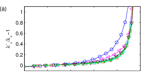
We first measure and for each intruder by using the depth, velocity, and acceleration data for all trajectories [11]. We then ask how these functions, shown in Fig. 7, are affected by the intruder shape, where we focus particularly on the triangular intruders. The static force term, , shown in the top panel of Fig. 7, is essentially insensitive to intruder shape, within the scatter of the data. In this figure, different colors distinguish the various intruders. By contrast, the collisional term, , shows significant dependence on shape (bottom panel). This term exhibits an initial transient, followed by roughly steady-state behavior. We define to be this steady-state value of after the initial transient. More elongated intruder noses (i.e., larger ) are associated with decreasing . The transition from the initial transient to corresponds roughly to the time at which the nose penetrates the granular material, and presumably to the formation of a steady-state velocity field around the intruder. The transient behavior also depends on the shape, where blunt-nosed intruders () have , and elongated-nosed intruders () have . Additionally, as discussed previously, we also measure using the calibrated photoelastic response starting after the nose is fully submerged. This allows us to examine the contributions made by different pieces of the intruder nose (i.e., the sides or the tip of the triangular nose).


Figure 8 shows a summary of the behavior of the velocity-squared drag coefficient, , and its dependence on shape for different intruders, as well as a comparison to the collisional model predictions in Eqs. (4) and (5). Specifically, the top of Figure 8 shows results for triangular-nosed intruders that demonstrate the two methods of calculating the total collisional drag coefficient: from the intruder trajectories (open, red circles) and using the photoelastic response (red dots). These two very different approaches are in good agreement with each other. Using the photoelastic data, shown in Figure 4, we decompose these drag coefficients into contributions from the sides (open, black squares), which matches well to the predictions for the collisional stresses with the flat surfaces of the triangular-nose intruders dependence (solid, black line), and contributions from the tip (blue crosses). These latter data asymptotically approach a constant value as the aspect ratio is increased from to (i.e., as the tip is made more prominent), which we capture with an approximate fit of . Considering the tip as a small flat section with a width of 3 mm, its contribution for large is approximately 10 times bigger than what occurs for a comparable area on the flat part of the intruders. The large contribution from the tip is visually clear by inspection of the photoelastic videos, which show a surprisingly large amount of acoustic pulses emanating from the intruder tip. (The examples shown in Figure 1 are representative of this). In this regard, we note that the model is based on an assumption of locally smooth surfaces such that the flux of clusters impinging on the surface is a coarse-grained measure. At the tip, this assumption is violated, implying that the tip needs to be treated on a separate footing.


In the bottom panel of Figure 8, we plot versus , also including data for circular- and elliptical-nosed intruders, from [11]. Since intruders with circular or elliptical noses are smooth (i.e., have no small tips), we use the value of extracted from the trajectories. In this figure, we have also plotted separately the contributions from the sides and from the tip of triangular-nosed intruders. There is a good linear collapse of all the data, except perhaps the heaviest circular-nosed intruder (see [11] for further discussion). The successful linear collapse of , which is measured from experimental data, versus , which is calculated from the theory, within an overall shape-independent constant, is a strong confirmation of the collisional model and is the first main result of this paper. This implies that , which contains the microscopic details for collisions, is relatively constant for all intruders used.
IV.2 Rotational Dynamics
Thus far, the collisional model has provided a good description of the vertical force on the intruder. We now examine the intruder rotations in the context of the collisional model, as in Eqs. (7) and (8). An image of an intruder which is rotated by an angle is shown in Fig. 9.

For the symmetric intruders used here,when , the integral is equal to zero (since and are both odd functions in , and everything else is even). However, as noted earlier, for , the integral in Eq. 8 is non-zero. To first order in , we can write:
| (9) |
where corresponds to intruders which are unstable to small perturbations in their angular orientation. Writing an equation for torque about the center of mass for small angles, and setting it equal to the moment of inertia, , times the angular acceleration, , yields:
| (10) |
where, .

Testing this relation nominally requires and . As for the motion of the intruder center of mass, the numerical computation of each time derivative of obtained from experiment amplifies the measurement noise. However, examination of the angular trajectories, vs. indicates approximately exponential growth: , as shown in Fig. 10. Thus, instead of directly testing Eq. 10, the data suggest that analyzing the angular orientation as a function of depth, might be a useful approach. In order to faciliate such analysis, we use product and chain rules, along with the decelerating force from Eq. 1, to write:
| (11) | |||||
Combining this result with Eq. (10) yields:
| (12) |
In the large-velocity regime (i.e., where the velocity-squared force dominates), the right-hand side of this equation is small, and, if is constant, this equation can be easily solved. Examining Figs. 5 and 7, we see that N for much of the trajectory (recall, the intruder mass is 0.219 kg), and right side is further reduced for large velocities by . Hence, for the moment, we assume that the right side of Eq. 12 is negligible (we return later to the validity of this approximation). Replacing with , we obtain:
| (13) |
where are constants of integration, and
| (14) |
For , the are purely real, with and . In this case, the collisional model predicts exponential growth in depth of the angle of rotation, with a growth rate . The quantities and , which yield , are straightforward to calculate from the intruder geometry, and is already calculated for the intruders used here (Figs. 7 and 8).
As noted, plots of the natural log of the angle versus depth follow approximately straight lines, where the slope corresponds to (Fig. 10). Leftward and rightward rotation are both plotted as positive. We measure the slope of these lines for all trajectories which break symmetry sufficiently (i.e., have at least 3000 data points where ) and which have initial velocities m/s. (This ensures that the right-hand side of Eq. 12 is small for the bulk of the trajectory). The resulting data for show reasonable reporducibility for each shape and initial velocity, and clear variations from one shape to another (bottom panel of Fig. 11). Note that no trajectories are plotted, as they do not show sufficient rotation. Moreover, rotational stability of the intruder is expected, since (top panel of Figure 11). For instance, when , a small perturbation of from zero will lead to behavior in time that will be roughly oscillatory. For instance, if we freeze , the resulting equation of motion is oscillatory. However, when , the dynamics are predicted to be saddle-like.


To compare these predictions to the experimental data, we calculate for the triangular intruders according to equations (7)-(14). Figure 12 is intended as a visual aid for the following discussion, as it depicts the geometrical quantities used in this calculation. We break the integral for into two sections for the left and right sides. We replace the terms involving with terms involving (the intruder nose angle) and ; specifically, and . This simplifies the calculation, yielding the torques for the left and right sides,
| (15) | |||||
| (16) | |||||
where the total torque in Eqs. (7) and (8) is then given by the difference between these two expressions. Here, is the distance from the nose-tail boundary to the center of mass as shown in Fig. 12. Positive is into the triangular nose, negative is into the rectangular tail, are the horizontal projections of the left and right sides of the triangular nose, and and are the strictly positive vertical and horizontal distances, respectively, from the center of mass to the midpoint of the sides of the triangular nose. The expressions for and are functions of area, , mass, , and width, , although we hold these quantities constant, as well as functions of the nose aspect ratio, which we vary in these experiments:
| (17) | |||||
| (18) | |||||
The contribution from the tip must also be included, since the force there can be substantial, e.g. Fig. 8. We model the tip force, , according to the dashed fit line in Figure 8, given by:
| (19) |
We assume this force always acts in the -direction, which allows a calculation of the torque from the tip, :
| (20) |
Finally, we obtain:
| (21) |
where we consider the small limit.
The top panel of Figure 11 shows a plot of versus aspect ratio, with (red line) and without (blue line) the contribution from the tip included. Recall from Eqs. (9) and (10) that corresponds to a rotational instability. Thus, with or without the tip contribution included, the instability occurs between and , which is consistent with the experimental data, as no intruders show substantial rotations. The value for is then used to calculate according to Eq. (14). Note also that there are no free parameters here, since the values of Ns2/m and , given by Eq. (19), are inputs from the collisional drag measurements shown in Fig. 7. The model prediction for is in good agreement with the experimental results, as shown in the bottom panel of Fig. 11. The dashed line shows the prediction without the tip contribution, while the solid line includes the tip. This constitutes the second main result of this paper.
Concerning the scatter in the data for measured values of , we suggest several possible explanations. First, we neglected the right-hand side of Eq. 12. In practice, this term is associated with a velocity- and depth-dependent correction to through the coefficient in front of . The strength of this correction depends on the velocity and depth at which the bulk of the rotation occurs. However, Fig. 13 shows that the error introduced into is small for approximately 80-90% of the trajectory. Thus, the data for exponential fits in Fig. 10 are primarily in the regime where the approximation made here is valid. Second, the collisional process which is responsible for rotations is stochastic (in time, in space, and in magnitude). Thus, we expect some fluctuations, especially when considering a single trajectory. Previous studies on the dynamics [10, 11] showed that the deceleration is highly fluctuating for individual trajectories, but for long times and many trajectories, it approaches the average behavior. Third, we assumed that the force from the tip always pointed directly upwards, but a horizontal component of the tip force could have a strong effect, particularly given the relatively large distance from the center of mass to the tip. Fourth, we assumed that the collisions were equally likely everywhere over the intruder surface. If this assumption is not strictly true, it would not substantially affect the velocity-squared drag, but it could have a stronger affect on the torque. However, on average, the collisional model captures the overall behavior of exponential growth, as well as the magnitude and scaling of the growth rate with intruder shape.

V Conclusions
In this paper, we have presented data for the dynamics of triangular-nosed intruders impinging on a granular bed from above. We found that the average dynamics are captured well by a macroscopic force law, Eq. (1), and that the magnitude of the velocity-squared drag force, , depends strongly on intruder shape, while the static term, , shows very little dependence on intruder shape. We also observed that intruder rotations become increasingly significant as the intruder nose is elongated, and that in such cases, the angle of the intruder grows approximately exponentially in depth, .
Additionally, we have proposed a collisional model for the velocity-squared drag on an intruder moving through a granular medium, and we have used experimental data to test this model. The key component in the model is momentum transfer from the intruder to the grains. By focusing on intruders with triangular noses, we are able to systematically explore the effect of intruder shape on the collision process. We observe experimentally that momentum transfer per unit surface length is larger at the tip than elsewhere along the sides of the intruders. By modeling the collision process in terms of both tip and side contributions, we observe excellent agreement with both the intruder deceleration and angular orientation. The agreement between these two linearly independent measurements of the mesoscopic collisional theory serves as an additional confirmation of the basic assumptions, which are as follows. The velocity squared drag and angular rotations:
- (a)
are dominated by intermittent, generally inelastic, collisions;
- (b)
collisions involve grain clusters which can be modeled by as having a fixed (mean) mass;
- (c)
collisions occur with equal probability throughout the granular material;
- (d)
momentum transfer acts normally inward at the site of collision on the intruder surface;
- (e)
there is a disproportionately larger contribution from collisions occuring at the tip of the intruder when is large.
We note several important aspects to the physics that underlie the model. First, the momentum transfer acts normally at the point of collision, which essentially says that friction between the grains and intruder is not important in this process [13]. The shape factors, and , were derived under this assumption, which is verified by the agreement with experimental data (shown in Figs. 8 and 11). We note that this is simply for the collisional term, which controls the velocity-squared drag and the corresponding off-axis rotations. Another point is that there is a force network that is dynamically excited by the intruder. If the network were to fail rapidly under the advance of an intruder, we would not expect to excite ‘clusters’, at least not in the same way as we observe in the experiments. Also of importance is the characteristic length of the force network that is excited by a single event. In Clark et al. [10], we found that this characteristic length was in the range of ten to a few tens of grains (note that this is consistent with our estimate of the cluster size from Fig. 2). It is interesting to contrast the collisional picture of Poncelet with Bagnold scaling [23] for shear flow, where shear stresses are expected to vary as due to inter-particle collisions, but in a much less dense granular phase. Finally, we note the relevance of the speed of the intruder (at impact and later) relative to the granular sound speed. In the present experiments, this ratio is small, no more than 0.02. As the intruder speed increases relative to the granular sound speed, the present model scenario may need modification. In particular, when the intruder speed is high enough, the force signal propagating into the material may not be able to ‘run away’ from the intruder. In any event, one might expect the typical cluster size in a collision event to grow as the impact speed approaches the granular sound speed.
An interesting question for both experiments and models concerns intruder dynamics in three dimensions. The fact that a number of 3D experiments with comparable impact and granular wave speeds also find scaling for the dynamic part of the drag suggests that a collisional model of the type developed here could be applied successfully to 3D. The fact that stresses from collisions can be determined within normalization suggests that it may be possible to use such an approach for applications, such as maximizing or minimizing the inertial drag or understanding the stability and dynamics of rotations of granular intruders as a function of intruder shape.
This work has been supported by the U.S. DTRA under Grant No. HDTRA1-10-0021. We very much appreciate additional input from Dr. L. Kondic, Dr. C. O’Hern, and Dr. W. Losert.
References
- [1] L. Euler, Neue Grundsätze der Artillerie, reprinted in Opera Omnia. (Druck und Verlag Von B.G. Teubner, Berlin, 1922).
- [2] J. V. Poncelet, Cours de Mécanique Industrielle. (Lithographie de Clouet, Paris, 1829).
- [3] W. A. Allen, E. B. Mayfield, and H. L. Morrison, J. Appl. Phys., 28, 370 (1957).
- [4] M. J. Forrestal and V. K. Luk, Int. J. Impact Eng. 12, 427 (1992).
- [5] L. Tsimring and D. Volfson, in Proceedings of the International Conference on Powders and Grains (Taylor & Francis, London, 2005), Vol 2, pp. 1215-1223.
- [6] H. Katsuragi and D. J. Durian, Nature Phys. 3, 420 (2007).
- [7] D. I. Goldman and P. Umbanhowar, Phys. Rev. E 77, 021308 (2008).
- [8] P. Umbanhowar and D. I. Goldman, Phys. Rev. E 82, 010301(R) (2010).
- [9] Y. Takehara, S. Fujimoto, and K. Okumura, Europhys. Lett. 92, 44003 (2010).
- [10] A. H. Clark, L. Kondic, and R. P. Behringer, Phys. Rev. Lett. 109, 238302 (2012).
- [11] A. H. Clark and R. P. Behringer, Europhys. Lett. 101 64001 (2013).
- [12] A. H. Clark, L. Kondic, and R. P. Behringer, in Proceedings of the International Conference on Powders and Grains (AIP Publishing LLC, 2013), Vol 1542, pp. 445-448.
- [13] A. Seguin, Y. Bertho, P. Gondret, and J. Crassous, Europhys. Lett. 88, 44002 (2009).
- [14] M. P. Ciamarra, A. H. Lara, A. T. Lee, D. I. Goldman, I. Vishik, and H. L. Swinney, Phys. Rev. Lett. 92, 194301 (2004).
- [15] M. A. Ambroso, C. R. Santore, A. R. Abate, and D. J. Durian, Phys. Rev. E 71, 051305 (2005).
- [16] J. R. de Bruyn and A. M. Walsh, Can. J. of Phys. 82, 439 (2004).
- [17] A. M. Walsh, K. E. Holloway, P. Habdas, and J. R. de Bruyn, Phys. Rev. Lett. 91, 104301 (2003).
- [18] E. L. Nelson, H. Katsuragi, P. Mayor, and D. J. Durian, Phys. Rev. Lett. 101, 068001 (2008).
- [19] K. A. Newhall and D. J. Durian, Phys. Rev. E 68, 060301(R) (2003).
- [20] T. A. Brzinski III, P. Mayor, and D. J. Durian, Phys. Rev. Lett. 111 168002 (2013).
- [21] I. Albert, J. G. Sample, A. J. Morss, S. Rajagopalan, A.-L. Barabási, and P. Schiffer,
- [22] J. Goldsmith, H. Guo, S. N. Hunt, M. Tao, and S. Koehler, Phys. Rev. E 88 030201(R) (2013).
- [23] R. A. Bagnold, Proc. R. Soc. London, Ser. A 255, 49 (1954).