跳到论文正文
W Papers独立论文阅读器 arXiv:1310.3047 论文正文 计算阅读时间 · 0%
引用这篇论文根据当前论文元数据生成,正式投稿前建议核对。


License: arXiv.org perpetual non-exclusive license
arXiv:1310.3047v2 [quant-ph] 14 Apr 2015

Quantum algorithm for universal implementation of projective measurement of energy

Shojun Nakayama Affiliation: Department of Physics, Graduate School of Science, University of Tokyo, 7-3-1, Hongo, Bunkyo-ku, Tokyo, Japan    Akihito Soeda Affiliation: Department of Physics, Graduate School of Science, University of Tokyo, 7-3-1, Hongo, Bunkyo-ku, Tokyo, Japan Affiliation: Centre for Quantum Technologies, National University of Singapore, Singapore    Mio Murao Affiliation: Department of Physics, Graduate School of Science, University of Tokyo, 7-3-1, Hongo, Bunkyo-ku, Tokyo, Japan Affiliation: Institute for Nano Quantum Information Electronics, University of Tokyo, 4-6-1, Komaba, Meguro-ku, Tokyo, Japan
Abstract

A projective measurement of energy (PME) on a quantum system is a quantum measurement, determined by the Hamiltonian of the system. PME protocols exist when the Hamiltonian is given in advance. Unknown Hamiltonians can be identified by quantum tomography, but the time cost to achieve a given accuracy increases exponentially with the size of the quantum system. In this letter, we improve the time cost by adapting quantum phase estimation, an algorithm designed for computational problems, to measurements on physical systems. We present a PME protocol without quantum tomography for Hamiltonians whose dimension and energy scale are given but otherwise unknown. Our protocol implements a PME to arbitrary accuracy without any dimension dependence on its time cost. We also show that another computational quantum algorithm may be used for efficient estimation of the energy scale. These algorithms show that computational quantum algorithms have applications beyond their original context with suitable modifications.

pacs
03.67.-a, 03.67.Ac, 06.20.Dk

I Introduction

Projective measurement of energy (PME) is a quantum counterpart of an ideal energy measurement in classical mechanics. A PME on a given system sets the system to an energy eigenstate and returns the corresponding energy eigenvalue. A PME alone has no effect on a system already in an energy eigenstate, thus can be used to confirm that the system remains in the initial energy eigenstate by repeating the same PME and observing that the outcomes remain unchanged. These properties make PME suitable for detecting small effects on a quantum system that is subject to an external influence such as gravity wave [1] or thermal fluctuation [2, 3, 4].

In practice, a device that implements a quantum measurement must include a destructive component such as a photon detector. PME being a nondestructive measurement requires another quantum system as a “probe”. The system (commonly referred to as “target”) interacts with the probe, and a direct measurement is performed only on the probe after the interaction (Fig. 1).

An implementation protocol of PME is known for systems whose Hamiltonian HH is given in advance [5]. The protocol chooses the interaction between the probe and target according to HH, so that the two quantum systems are appropriately entangled. The entanglement assures that the measurement on the probe sets the target to an energy eigenstate, and that the outcome of the measurement identifies the respective energy eigenvalue. The time needed to induce the entanglement can be made arbitrarily short by increasing the strength of the interaction. Thus, PME of known HH can be implemented instantaneously in principle.

Refer to caption
Figure 1: (Color online) Schematic diagrams of PME protocols on a system of unknown self-Hamiltonian HH (labeled “Target”). The blue boxes exp⁡(−i​H​t)\exp(-iHt) denote the target being let evolve for time tt with ℏ=1\hbar\!=\!1. M is a quantum measurement which returns a numerical outcome. The implementation time is lower-bounded by the time required to induce the evolution of the target system, since there is no limit to the strength of the interaction induced from outside on the system in principle. In the top protocol, HH is identified by quantum (process) tomography, with at least NQ​T=O⁡(d2)N_{QT}=O(d^{2}) uses of the time evolution exp⁡(−i​H​t)\exp(-iHt) for dd-dimensional systems. The quantum algorithmic PME (bottom) proposed in this letter avoids quantum tomography and all interactions are HH-independent.

This protocol, however, does not take into account the time required to identify HH. Let us estimate the time cost by analyzing quantum process tomography [6, 7] on the time evolution of the system. Process tomography involves setting the target to various “test states” and measuring the expectation value of appropriate observables for each resulting state after the time evolution. A complete process tomography for a system described by a dd-dimensional Hilbert space ℋ=ℂd\mathcal{H}=\mathbb{C}^{d} requires a number of observable, O⁡(d2)O(d^{2}), equal to the number of parameters in the Hamiltonian [8].

An accurate estimation of the expectation values needs to accumulate sufficient statistics. Each use of the time evolution costs time tt, hence the total time cost for the tomography to achieve a given accuracy for a dd-dimensional system scales at least O⁡(d2)O(d^{2}). This implies that, if HH is unknown, the total implementation time for PME via process tomography grows at least exponentially in the number of subsystems due to the exponential growth of the total dimension for composite systems.

Tomography is required even if a PME is to be performed only once. It extracts enough information to identify all the eigenspaces and eigenvalues of HH, so the dimension dependence is unavoidable. A single use of PME, however, does not reveal the exact description of the energy eigenspaces or the whole energy spectrum. A more efficient PME protocol is needed.

To improve a PME protocol is to find a better quantum algorithm. Some quantum algorithms are known to provide an efficient solution to computational problems [9]. These algorithms, however, assume that the dynamics of a quantum system can be “switched off” at will, which does not hold in this problem.

In this paper, we introduce a more efficient PME protocol and show that we can remove the dimension-dependence in the time cost, for unknown Hamiltonians whose energy scale is given. Our protocol exploits a modified version of quantum phase estimation (QPE) [10]. Finally, we discuss an estimation protocol for the energy scale, based on an estimation of the trace of a unitary operator. We will show that another computational quantum algorithm, adapted from Ref. [11], performs more efficiently than a complete tomography.

II Projective measurement by QPE

QPE is designed so that each run returns a good estimate for some eigenvalue of a given unitary operator U=∑k=1dexp⁡(i​θk)​|θk⟩​⟨θk|U=\sum_{k=1}^{d}\exp(i\theta_{k})|{\theta_{k}}\rangle\langle{\theta_{k}}| on ℋ=ℂd\mathcal{H}=\mathbb{C}^{d}. Note that we assume 0≤θk<2​π0\leq\theta_{k}<2\pi. For a given input state |θk⟩|{\theta_{k}}\rangle, the corresponding phase θk\theta_{k} is estimated by QPE.

An essential building block of QPE is a controlled-unitary operation CUC_{U}, which is a unitary gate that conditionally operates UU on a dd-dimensional target system denoted by ℋt=ℂd\mathcal{H}_{t}=\mathbb{C}^{d} according to the state of an extra control qubit denoted by ℋc=ℂ2\mathcal{H}_{c}=\mathbb{C}^{2}. Formally, the action of CUC_{U} on ℋc⊗ℋt\mathcal{H}_{c}\otimes\mathcal{H}_{t} is defined by CU​|0⟩​|φ⟩=|0⟩​|φ⟩C_{U}|{0}\rangle|{\varphi}\rangle\!=\!|{0}\rangle|{\varphi}\rangle and CU​|1⟩​|φ⟩=|1⟩​U​|φ⟩C_{U}|{1}\rangle|{\varphi}\rangle\!=\!|{1}\rangle U|{\varphi}\rangle for any |φ⟩∈ℋt|{\varphi}\rangle\in\mathcal{H}_{t} where {|0⟩,|1⟩}\{|{0}\rangle,|{1}\rangle\} forms the computational basis of ℋc\mathcal{H}_{c}. To achieve NN-bits estimation, QPE uses NN control qubits for applying (CU)2l−1(C_{U})^{2^{l-1}} between the ll-th control qubit for each l∈{1,…,N}l\in\{1,\dots,N\} and the target. We obtain an NN-bit string {n1,⋯,nN}\{n_{1},\cdots,n_{N}\} of outcomes by the final measurements on the NN control qubits in the computational basis. By defining 𝐧N:=∑l=1N2l−1​nl\mathbf{n}_{N}:=\sum_{l=1}^{N}2^{l-1}n_{l} and f⁡(𝐧N):=𝐧N/2Nf(\mathbf{n}_{N}):=\mathbf{n}_{N}/2^{N}, the phase θk\theta_{k} is estimated as θk=2​π​f​(𝐧N)\theta_{k}=2\pi f(\mathbf{n}_{N}).

In the limit N→∞N\rightarrow\infty, f⁡(𝐧N)f(\mathbf{n}_{N}) can be regarded as a continuous variable ff with 0≤f≤10\leq f\leq 1. For any θk\theta_{k}, the probability pN​(f⁡(𝐧N)|θk)p_{N}(f(\mathbf{n}_{N})|\theta_{k}) to obtain 𝐧N\mathbf{n}_{N} for an initial state |θk⟩|{\theta_{k}}\rangle approaches the delta function δ⁡(f−θk/2​π)\delta(f-\theta_{k}/2\pi) in distribution. The distance between pN​(f⁡(𝐧N)|θk)p_{N}(f(\mathbf{n}_{N})|\theta_{k}) and δ⁡(f−θk/2​π)\delta(f-\theta_{k}/2\pi) is independent of dd. At the same limit, the target is transformed to an eigenstate by a projection onto the corresponding eigenspace induced by the final measurements of QPE. Interested readers may refer to Appendix. A for details of QPE.

III QPE and universal controllization

The evolution of a target with Hamiltonian HH for time tt is given by the unitary operator U⁡(t)=exp⁡(−i​H​t)U(t)=\exp(-iHt), with ℏ=1\hbar=1. It may appear that QP on U⁡(t)U(t) readily implements a projection onto the eigenspace corresponding to the estimated phase of U⁡(t)U(t), which is also the desired PME of HH up to ambiguity due to the phase periodicity. QPE assumes that UU is available in its quantum-controlled form, namely, CUC_{U}, but the time evolution operator is not. Adding a quantum control to a quantum gate– a task which we call controllization– is not trivial when UU is unknown. In this paper we introduce universal controllization, a quantum subroutine that approximately implements controllization for unknown UU.

We introduce a dd-dimensional ancillary system denoted by ℋa=ℂd\mathcal{H}_{a}=\mathbb{C}^{d} and define a unitary gate WU:=CS​(𝕀2⊗U⊗𝕀d)​CSW_{U}:=C_{S}\left({\mathbb{I}}_{2}\otimes U\otimes{\mathbb{I}}_{d}\right)C_{S} on ℋc⊗ℋt⊗ℋa\mathcal{H}_{c}\otimes\mathcal{H}_{t}\otimes\mathcal{H}_{a} where CSC_{S} is a unitary gate called the controlled-swap operation defined by CS​|0⟩​|ψ⟩​|ϕ⟩=|0⟩​|ϕ⟩​|ψ⟩C_{S}|{0}\rangle|{\psi}\rangle|{\phi}\rangle\!=\!|{0}\rangle|{\phi}\rangle|{\psi}\rangle and CS​|1⟩​|ψ⟩​|ϕ⟩=|1⟩​|ψ⟩​|ϕ⟩C_{S}|{1}\rangle|{\psi}\rangle|{\phi}\rangle\!=\!|{1}\rangle|{\psi}\rangle|{\phi}\rangle, for any |ψ⟩,|ϕ⟩∈ℂd|{\psi}\rangle,|{\phi}\rangle\!\in\!{\mathbb{C}}^{d}, and 𝕀k\mathbb{I}_{k} denotes the k×kk\times k identity matrix. We call WUW_{U} a classically conditioned quantum gate since it perfectly simulates CUC_{U} when the control qubit is in a state |0⟩|{0}\rangle or |1⟩|{1}\rangle. But WUW_{U} deviates from CUC_{U} for a general input state |η⟩=α​|0⟩+β​|1⟩|{\eta}\rangle=\alpha|{0}\rangle+\beta|{1}\rangle in the control. Since WU​|η⟩​|ψ⟩​|ϕ⟩=α⁡|0⟩​|ψ⟩​U​|ϕ⟩+β⁡|1⟩​U​|ψ⟩​|ϕ⟩W_{U}|{\eta}\rangle|{\psi}\rangle|{\phi}\rangle\!=\!\alpha|{0}\rangle|{\psi}\rangle U|{\phi}\rangle\!+\!\beta|{1}\rangle U|{\psi}\rangle|{\phi}\rangle, the ancilla system is also entangled to the control and target systems and thus decoherence occurs in the control-target system in general. If we can prepare an eigenstate of UU in the ancilla system, exact implementations of CUC_{U} is possible [14, 12, 13], but such implementations require knowledge on UU. Other know controllization schemes  [16, 15] also require that the quantum gate is at least partially known.

It is even proven that an exact controllization is impossible within quantum mechanics [17, 14]. These results are derived assuming that the input quantum gate is a blackbox. The unitary operator U⁡(t)U(t), on the other hand, has a tunable parameter, namely, the evolution duration tt. We exploit this feature and a decoupling method [18] used in quantum information theory to asymptotically implement a universal controllization of U⁡(t)U(t). The implementation accuracy of our controllization depends on the maximum difference between any two eigenvalues of HH.

To reduce the decoherence by WUW_{U}, we need to make the resulting state of the ancilla depend as little as possible on the initial control-target state. Let us prepare the ancilla in the completely mixed state 𝕀d/d{\mathbb{I}}_{d}/d, so that the state of the ancilla remains the same at least when the control qubit is in |0⟩|{0}\rangle or |1⟩|{1}\rangle for any given UU. We consider the reduced map on the control-target system,

ΓU​[ρ]:=Trℋa​[WU​(ρ⊗𝕀d/d)​WU†],\Gamma_{U}\left[\rho\right]:=\mathrm{Tr}_{{\mathcal{H}}_{a}}\left[{W_{U}(\rho\otimes{\mathbb{I}}_{d}/d)W_{U}^{\dagger}}\right], (1)

where ρ\rho is a density matrix on ℂ2⊗ℋt\mathbb{C}^{2}\otimes\mathcal{H}_{t}. We call the map ΓU\Gamma_{U} as pseudo controllization. For ρ=|η⟩​⟨η|⊗|ψ⟩​⟨ψ|\rho=|{\eta}\rangle\langle{\eta}|\otimes|{\psi}\rangle\langle{\psi}|, we have

ΓU​[|η⟩​⟨η|⊗|ψ⟩​⟨ψ|]=CU​(|η⟩​⟨η|⊗|ψ⟩​⟨ψ|)​CU†+[αβ∗|0⟩⟨1|⊗|ψ⟩⟨ψ|(γU−1)U†+c.c.],\Gamma_{U}\left[|{\eta}\rangle\langle{\eta}|\otimes|{\psi}\rangle\langle{\psi}|\right]=C_{U}\left(|{\eta}\rangle\langle{\eta}|\otimes|{\psi}\rangle\langle{\psi}|\right)C_{U}^{\dagger}+\\ \left[\alpha\beta^{*}|{0}\rangle\langle{1}|\otimes|{\psi}\rangle\langle{\psi}|\left(\gamma_{U}-1\right)U^{\dagger}+c.c.\right], (2)

where γU=Tr⁡[U]/d\gamma_{U}=\mathrm{Tr}\left[{U}\right]/d. The second term in Eq. (2) acts as a kind of phase damping noise on the control-target system. The factor γU−1\gamma_{U}-1 determines the deviation of the reduced map ΓU\Gamma_{U} from the ideal controllization. We define the coherence factor aU:=|γU|a_{U}:=|\gamma_{U}| and a phase factor ei​φU:=γU/|γU|e^{i\varphi_{U}}:=\gamma_{U}/|\gamma_{U}|. Notice that 1−aU≤|γU−1|1-a_{U}\leq\left|\gamma_{U}-1\right|. Thus, the phase damping noise is minimized if we regard ΓU\Gamma_{U} as an approximation of CU′C_{U^{\prime}} for U′=e−i​φU​UU^{\prime}=e^{-i\varphi_{U}}U. In a sense, ΓU\Gamma_{U} implements a noisy controlled-unitary operation, where the magnitude of the noise is determined by a positive quantity −aU1\!-\!a_{U}.

We further reduce the dependence of the ancilla on the initial control-target state by use of a set {σr}\{\sigma_{r}\} of unitary operations on the ancilla such that

1d2​∑rσr​WU​(ρtot⊗𝕀d/d)​WU†​σr†=ΓU​[ρtot]⊗𝕀d/d.\frac{1}{d^{2}}\sum_{r}\sigma_{r}W_{U}(\rho_{\rm tot}\otimes{\mathbb{I}}_{d}/d)W_{U}^{\dagger}\sigma_{r}^{\dagger}=\Gamma_{U}\left[\rho_{\rm tot}\right]\otimes{\mathbb{I}}_{d}/d. (3)

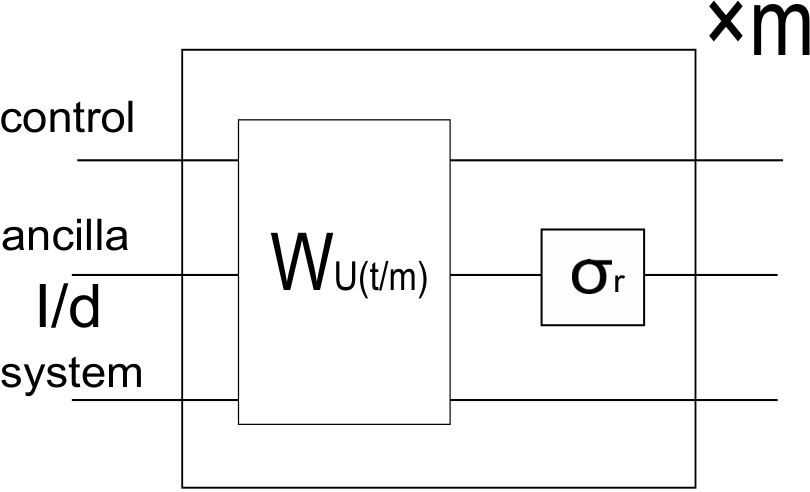
Note that the ancilla is “refreshed” to the completely mixed state only by operations on the aniclla. (Such a random operation has been extensively applied to questions in quantum communication [18].) We divide WU⁡(t)W_{U(t)} into mm repetitions of WU⁡(t/m)W_{U(t/m)}, each followed by the refreshing operation (3). Here, mm fixes the refresh rate. The strength of the noise after each refreshing operation is O⁡(1m2)O(\frac{1}{m^{2}}). Thus the total effect of the noise scales O⁡(m×1m2)=O⁡(1m)O(m\!\times\!\frac{1}{m^{2}})=O(\frac{1}{m}), which vanishes in the asymptotic limit of m→∞m\rightarrow\infty . (see Appendix. B.4, for details). This phenomenon is mathematically analogous to the quantum Zeno effect [19].

We call this asymptotic implementation of a controlled-unitary operation including the repeated refreshing operation, universal controllization. For finite mm, the universal controllization approximates the controlled-unitary operation CU[m]​(t)C_{U^{[m]}(t)}, where U[m]​(t)=e−i​m​φU⁡(t/m)​U​(t)U^{[m]}(t)\!=\!e^{-im\varphi_{U(t/m)}}U(t). With m→∞m\!\rightarrow\!\infty, exp⁡(i​m​φU⁡(t/m))\exp(im\varphi_{U(t/m)}) converges to exp(−iTr[H]t/d)\exp(-i\mathrm{Tr}\left[{H}\right]t/d). In a sense, universal controllization fixes the reference point of the energy of HH so that Tr⁡[H]=0\mathrm{Tr}\left[{H}\right]=0. A more detailed discussion of universal controllization is presented in Appendix. B.

IV PME by universal controllization

A perfect PME for a system with a Hamiltonian HH is distinguished from other quantum operations by two properties. First, the system remains in the same eigenstate when a PME is applied consecutively. Second, the outcomes of the consecutive measurements are all precisely equal to EkE_{k}. The probability density p⁡(E|Ek)p(E|E_{k}) of obtaining EE as the outcome must be the delta function δ⁡(E,Ek):=δ⁡(E−Ek)\delta(E;E_{k}):=\delta(E-E_{k}). Conversely, the only measurement satisfying these properties is a perfect PME.

A subtlety is that a perfect PME for HH and for H−λ​𝕀H-\lambda\mathbb{I} should be considered equivalent, since two Hamiltonians with different reference points of energy are physically equivalent. A measurement scheme is regarded as a perfect PME for HH if p⁡(E|Ek)=δ⁡(E,Ek−λ)p(E|E_{k})=\delta(E;E_{k}-\lambda) as long as λ\lambda is independent of kk.

Our PME protocol uses QPE on the time evolution operator U⁡(t)U(t) with CU[m]​(t)C_{U^{[m]}(t)} implemented by universal controllization. Here, the control qubits and ancilla of the universal controllization serve as the probe. The probe-target interaction is used to perform WU⁡(t/m)W_{U(t/m)}, the refreshing operations, and QFT. The lower figure in Fig. 1 provides a conceptual diagram.

In the ideal case of m→∞m\rightarrow\infty and N→∞N\rightarrow\infty, the modified QPE implements the projective measurement defined by the spectral decomposition of U~​(t)=exp⁡(−i​H~​t)\tilde{U}(t)=\exp\big(-i\tilde{H}t\big), where H~:=H−Tr⁡[H]​𝕀\tilde{H}:=H-\mathrm{Tr}\left[{H}\right]\mathbb{I}. The outcome ff gives −E~k​t(mod2​π)-\tilde{E}_{k}t\,\pmod{2\pi} for some energy eigenvalue E~k\tilde{E}_{k} of H~\tilde{H}.

E~k\tilde{E}_{k} cannot be uniquely determined from ff for general tt due to the periodicity of the phase function exp⁡(i​θ)\exp(i\theta). Let us restrict tt so that E~k∈(π/t,−π/t)\tilde{E}_{k}\in(\pi/t,-\pi/t), namely,

Δmax​t≤π/2,\Delta_{\mathrm{max}}t\leq\pi/2, (4)

where Δmax=maxk,l⁡|E~k−E~l|\Delta_{\mathrm{max}}=\max_{k,l}\big|\tilde{E}_{k}-\tilde{E}_{l}\big|. The energy eigenvalues are uniquely determined by

E⁡[f]={−2πf/tf∈[0,12)−(2πf−2π)/tf∈[12,1).E[f]=\begin{cases}-2\pi f/t&f\in\big[0,\frac{1}{2}\big)\\ -(2\pi f\!-\!2\pi)/t&f\in\big[\frac{1}{2},1\big)\end{cases}. (5)

Recall that the probability distribution of ff is the delta function δ⁡(f−θk/2​π)\delta(f\!-\!\theta_{k}/2\pi). Thus, p⁡(E|Ek)=δ⁡(E,Ek−Tr⁡[H])p(E|E_{k})=\delta(E;E_{k}\!-\!\mathrm{Tr}\left[{H}\right]), which is the desired function. The projection onto the corresponding energy eigenspace is already guaranteed by QPE.

For finite mm and NN, we continue to choose tt according to Eq. (4) and estimate EkE_{k} by Eq. (5) with ff replaced by f⁡(𝐧N)f(\mathbf{n}_{N}). The implemented measurement is an approximation of a PME. A target initially in an energy eigenstate |Ek⟩|{E_{k}}\rangle results in the same state at the end of the scheme. One of the conditions for a perfect PME is still satisfied. Thus, the accuracy of the scheme is determined by how close p⁡(E|Ek)p(E|E_{k}) for each |Ek⟩|{E_{k}}\rangle simulates a delta function δ⁡(E,Ek−λ)\delta(E;E_{k}-\lambda).

V Implementation accuracy and time cost

Recall that pN​(f⁡(𝐧N)|θk)p_{N}(f(\mathbf{n}_{N})|\theta_{k}) in QPE needs to approach the delta function δ⁡(f−θk/2​π)\delta(f-\theta_{k}/2\pi) in N→∞N\rightarrow\infty to achieve the projective measurement determined by UU. If each CUC_{U} in QPE is replaced by the adapted classical controllization (i.e., substituted by WUW_{U} and an ancilla), pN​(f⁡(𝐧N)|θk)p_{N}(f(\mathbf{n}_{N})|\theta_{k}) does not converge to the delta function unless aU=1a_{U}=1.

Let us denote by pN[m]​(f⁡(𝐧N)|Ek)p^{[m]}_{N}(f(\mathbf{n}_{N})|E_{k}) the probability distribution of f⁡(𝐧N)f(\mathbf{n}_{N}) for a given mm, NN, and initial state |Ek⟩|{E_{k}}\rangle. For a finite mm, the universal controllization approximately controllizes U′=exp⁡(−i⁡(H​t−m​φU⁡(t/m)​𝕀))U^{\prime}=\exp(-i(Ht\!-\!m\varphi_{U(t/m)}\mathbb{I})). In this case, each run of the approximated QPE provides an estimate for the eigenvalue corresponding to |Ek⟩|{E_{k}}\rangle, which is θk′=−Ek​t+m​φU⁡(t/m)(mod2​π)\theta^{\prime}_{k}\!=\!-E_{k}t\!+\!m\varphi_{U(t/m)}\pmod{2\pi}. When NN increases, the deviation of pN[m]​(f⁡(𝐧N)|Ek)p^{[m]}_{N}(f(\mathbf{n}_{N})|E_{k}) from pN​(f⁡(𝐧N)|θk′)p_{N}(f(\mathbf{n}_{N})|\theta^{\prime}_{k}) caused by the controllization error prevents the function converging to a delta function. (See Fig. 2.a) The deviation can be bounded by |pN[m]​(f⁡(𝐧N)|Ek)−pN​(f⁡(𝐧N)|θk′)|≤ϵ\left|p^{[m]}_{N}(f(\mathbf{n}_{N})|E_{k})-p_{N}(f(\mathbf{n}_{N})|\theta^{\prime}_{k})\right|\!\leq\!\epsilon for any ϵ>0\epsilon\!>\!0 when mm is set to

m≥(Δmax​t)2​N​2N−3/ϵm\geq(\Delta_{\mathrm{max}}t)^{2}N2^{N-3}/\epsilon (6)

as shown in Appendix. D.2.(See Fig. 2 b for examples.)

Refer to caption
(a) pN[m]​(f⁡(𝐧N)|Ek)p^{[m]}_{N}(f(\mathbf{n}_{N})|E_{k}) for a fixed mm
Refer to caption
(b) pN[m]​(f⁡(𝐧N)|Ek)p^{[m]}_{N}(f(\mathbf{n}_{N})|E_{k}) for an adaptively chosen mm
Figure 2: (Color online) Plots of probability distributions pN[m]​(f⁡(𝐧N)|Ek)p^{[m]}_{N}(f(\mathbf{n}_{N})|E_{k}) and their envelope functions for target Hamiltonian H=−∑λ=03|E0(λ)⟩⟨E0(λ)|+|E1⟩⟨E1|H\!=\!-\sum_{\lambda=0}^{3}|{E_{0}^{(\lambda)}}\rangle\langle{E^{(\lambda)}_{0}}|\!+|{E_{1}}\rangle\langle{E_{1}}|, t=⋅πt\!=\!0.225\!\cdot\!\pi, and setting Ek=E1E_{k}\!=\!E_{1}. Each marker represents pN[m]​(f⁡(𝐧N)|Ek)p^{[m]}_{N}(f(\mathbf{n}_{N})|E_{k}) of finding each outcome by a single round of the PME scheme. Fig.2 (a) presents pN[m]​(f⁡(𝐧N)|Ek)p^{[m]}_{N}(f(\mathbf{n}_{N})|E_{k}) for N=2,4,6N=2,4,6 for a fixed refreshing rate m=8m=8. Fig.2 (b) presents pN[m]​(f⁡(𝐧N)|Ek)p^{[m]}_{N}(f(\mathbf{n}_{N})|E_{k}) for N=2,4,6N=2,4,6 where each value of mm is adoptively chosen as a smallest integer satisfying m≥(Δmax​t)2​N​2N−3/ϵm\geq(\Delta_{\mathrm{max}}t)^{2}N2^{N-3}/\epsilon and target error ϵ\epsilon is set to 0.250.25. In all cases, markers corresponding to probability less than one tenth of the target error (0.0250.025) are omitted for clarity.

For a given refresh rate mm, each universal controllization makes mm uses of WU⁡(t/m)W_{U(t/m)}, where the total evolution duration (t/m)×m=t(t/m)\!\times\!m\!=\!t is independent of mm. Hence, pN[m]​(f⁡(𝐧N)|Ek)p^{[m]}_{N}(f(\mathbf{n}_{N})|E_{k}) can be brought arbitrarily close to pN​(f⁡(𝐧N)|θk′)p_{N}(f(\mathbf{n}_{N})|\theta^{\prime}_{k}) without increasing the time cost. The distribution pN​(f⁡(𝐧N)|θk′)p_{N}(f(\mathbf{n}_{N})|\theta^{\prime}_{k}) is not a delta function for any finite NN even with perfect controlled-unitary operations CUC_{U} (i.e., infinite mm). The cost doubles for each control qubit added, but the distance between pN​(f⁡(𝐧N)|θk′)p_{N}(f(\mathbf{n}_{N})|\theta^{\prime}_{k}) and the delta function δ⁡(E,E~k)\delta(E;\tilde{E}_{k}) is independent of the dimension of the target. Hence, the implementation accuracy of PME can be improved without any dimension dependence.

VI Quantum algorithmic estimation of the energy scale

We showed the existence of our PME protocol under the assumption that Δmax\Delta_{\mathrm{max}} is known. The assumption can be relaxed to knowing an upper bound on Δmax\Delta_{\mathrm{max}}. The bound may be estimated by quantum (process) tomography, but the tomography requires that a prior distribution of HH is given. For a certain prior distribution, it is possible to estimate the bound by measuring the coherence factor aUa_{U}. We observe that aUa_{U} approaches 11 as the product Δmax​t\Delta_{\mathrm{max}}t decreases to 00. Thus, when aUa_{U} is estimated to be close to 1, it is possible that Δmax​t\Delta_{\mathrm{max}}t is sufficiently small. While this is not true for some Hamiltonians, the probability of such “error” decreases exponentially in the dimension dd of the target for a particular class of prior distribution (see Appendix. E). Hence, we can reliably estimate aUa_{U}.

To estimate aUa_{U}, we modify the quantum algorithm presented in Ref. [11]. The original algorithm outputs the trace Tr⁡[U]\mathrm{Tr}\left[{U}\right] of an input unitary UU, provided that the corresponding CUC_{U} is available. In our problem, we replace CUC_{U} with WUW_{U}. With this modification, the original algorithm returns |Tr⁡[U]|2|\mathrm{Tr}\left[{U}\right]|^{2} (See Appendix. E.2, for details), thus we obtain aUa_{U} since aU2=|Tr⁡[U]|2/d2a_{U}^{2}\!=\!|\mathrm{Tr}\left[{U}\right]|^{2}/d^{2}. Clearly, this modified algorithm estimates aUa_{U} much more efficiently than process tomography.

Conclusion.—In this letter, we presented an implementation protocol for a projective measurement of energy on a system driven by an unknown Hamiltonian with a given energy scale. The implementation time cost of the protocol is independent of the dimension of the system unlike the one based on quantum process tomography. The protocol is based on a computational quantum algorithm called quantum phase estimation (QPE). We introduced universal controllization to make the computational algorithm executable without stopping the evolution of the target system. Another computational quantum algorithm is shown to be effective in estimating the energy scale with a suitable modification. This motivates the search for further applications of quantum algorithms outside their original computational context.

Acknowledgments: The authors thank T. Sugiyama and H. Nishimura for their insights and expertise. This work is supported by the Project for Developing Innovation Systems of MEXT, Japan, the Global COE Program of MEXT Japan, and JSPS KAKENHI (Grant No. 23540463, No. 23240001, and No. 26330006). The authors also gratefully acknowledge the ELC project (Grant-in-Aid for Scientific Research on Innovative Areas MEXT KAKENHI (Grant No. 24106009)) for encouraging the research presented in this paper. After the completion of our work, we were notified that our algorithm for calculating |Tr⁡[U⁡(t)]||\mathrm{Tr}\left[{U(t)}\right]| based on DQC1 has been independently discovered by J. Thompson, M. Gu, K. Modi, and V. Vedral in “Quantum Computing with Black-box Subroutines” [20]. We thank these authors for drawing their work to our attention.

Appendix A Elements of quantum phase estimation

This section provides details of quantum phase estimation (QPE) described in the second and the third sections in the main article on Projective measurement by QPE and QPE and universal controllization. QPE plays a crucial role in our protocol for projective measurement of energy (PME). A quantum circuit representation of the algorithm of QPE, the probability distribution of outcomes and the transformed state corresponding to each outcome by QPE are presented in Sec. A.1. In the main paper, we referred that the probability distribution of the outcome converges to a delta function at the limit where the number of control qubits goes infinity. In Sec. A.2, we give the mathematical formulation of the statement.

A.1 Probability distribution of outcomes and state change induced by QPE

QPE is designed so that each run returns a good estimate for one of the eigenvalues of a given unitary operator UU. QPE (originally proposed in [10]) is usually described in the state-vector formalism. In this subsection, we provide another description based on the density-matrix formalism to facilitate the comparison with the approximate QPE using universal controllization presented in Appendix. D.1.

The circuit representation of QPE is given in Fig. 3. Consider a target system ℂd{\mathbb{C}}^{d} and a control system consisting of NN-qubit systems ℂ2N{\mathbb{C}}^{2^{N}}. We set a basis of a qubit system ℂ2\mathbb{C}^{2} and denote the basis by {|0⟩,|1⟩}\{|{0}\rangle,|{1}\rangle\}.

First, we initialize the control and target system as

|0​…​0⟩​⟨0​…​0|⊗|θk⟩​⟨θk|,|{0\dots 0}\rangle\langle{0\dots 0}|\otimes|{\theta_{k}}\rangle\langle{\theta_{k}}|, (7)

on ℂ2N⊗ℂd\mathbb{C}^{2^{N}}\otimes{\mathbb{C}}^{d}, where |0…0⟩:=|0⟩⊗⋯⊗|0⟩|{0\dots 0}\rangle:=|{0}\rangle\otimes\cdots\otimes|{0}\rangle and |θk⟩|{\theta_{k}}\rangle is an eigenvector corresponding to eigenvalue ei​θke^{i\theta_{k}} of UU. The Hadamard gate H\mathrm{H} is then applied to each control qubit. Note that H\mathrm{H} achieves

H​|0⟩\displaystyle\mathrm{H}|{0}\rangle =(|0⟩+|1⟩)/2,\displaystyle=(|{0}\rangle+|{1}\rangle)/\sqrt{2}, (8)
H​|1⟩\displaystyle\mathrm{H}|{1}\rangle =(|0⟩−|1⟩)/2.\displaystyle=(|{0}\rangle-|{1}\rangle)/\sqrt{2}. (9)

The state after this operation is given by

12N​∑a1,a2,…​aNb1,b2,…,bN|a1​a2​…​aN⟩​⟨b1​b2​…​bN|⊗|θk⟩​⟨θk|,\frac{1}{2^{N}}\sum_{\begin{subarray}{a}a_{1},a_{2},\dots a_{N}\\ b_{1},b_{2},\dots,b_{N}\end{subarray}}|{a_{1}a_{2}\dots a_{N}}\rangle\langle{b_{1}b_{2}\dots b_{N}}|\otimes|{\theta_{k}}\rangle\langle{\theta_{k}}|, (10)

where al,bl∈{0,1}a_{l},b_{l}\in\{0,1\}.

A controlled-unitary operation CUC_{U} of an unitary operation UU is defined as

CU:=|0⟩​⟨0|⊗𝕀d+|1⟩​⟨1|⊗U\displaystyle C_{U}:=|{0}\rangle\langle{0}|\otimes\mathbb{I}_{d}+|{1}\rangle\langle{1}|\otimes U (11)

on ℂ2⊗ℂd{\mathbb{C}}^{2}\otimes{\mathbb{C}}^{d}. Here, 𝕀d\mathbb{I}_{d} denotes the d×dd\times d identity matrix. The superoperator representation 𝒞U\mathcal{C}_{U}, corresponding to CUC_{U}, is defined as

𝒞U​[ρ]:=CU​ρ​CU†.\mathcal{C}_{U}\left[\rho\right]:=C_{U}\rho C_{U}^{\dagger}. (12)

We choose the ll-th control qubit and the target system and apply the controlled-unitary operation 𝒞U2l−1\mathcal{C}_{U^{2^{l-1}}} for all 1≤l≤N1\leq l\leq N. This transforms the state to

12N​∑a1,a2,…​aNb1,b2,…,bN∏l=1Nexp⁡(i​2l−1​(al−bl)​θk)×|a1​a2​…​aN⟩​⟨b1​b2​…​bN|⊗|θk⟩​⟨θk|.\frac{1}{2^{N}}\sum_{\begin{subarray}{a}a_{1},a_{2},\dots a_{N}\\ b_{1},b_{2},\dots,b_{N}\end{subarray}}\prod_{l=1}^{N}\exp\left(i2^{l-1}(a_{l}-b_{l})\theta_{k}\right)\\ \times|{a_{1}a_{2}\dots a_{N}}\rangle\langle{b_{1}b_{2}\dots b_{N}}|\otimes|{\theta_{k}}\rangle\langle{\theta_{k}}|. (13)
Figure 3: A quantum circuit representation of QPE. The box QFT denotes the quantum Fourier transformation. The final measurement is performed in the computational basis.

Finally, the quantum Fourier transformation is applied and then the control qubits are measured in the computational basis

{|𝐧N⟩=|n1​n2​…​nN⟩|𝐧N=∑l=1Nnl⋅2l−1}.\left\{|{\mathbf{n}_{N}}\rangle=|{n_{1}n_{2}\dots n_{N}}\rangle\Big|\mathbf{n}_{N}=\sum_{l=1}^{N}n_{l}\cdot 2^{l-1}\right\}. (14)

The Fourier transformation and the measurement in the computational basis together are equivalent to performing a projective measurement on the state (13) in the Fourier basis, i.e.,

{|f⁡(𝐧N)⟩|0≤𝐧N<2N},\left\{|{f(\mathbf{n}_{N})}\rangle|0\leq\mathbf{n}_{N}<2^{N}\right\}, (15)

where f⁡(𝐧N):=𝐧N/2Nf(\mathbf{n}_{N}):=\mathbf{n}_{N}/2^{N} and

|f⁡(𝐧N)⟩:=∑𝐧N′=02N−1exp⁡(i​2​π​f​(𝐧N)​𝐧N′)2N​|𝐧N′⟩.|{f(\mathbf{n}_{N})}\rangle:=\sum_{\mathbf{n}^{\prime}_{N}=0}^{2^{N}-1}\frac{\exp\left({i2\pi f(\mathbf{n}_{N})\mathbf{n}^{\prime}_{N}}\right)}{\sqrt{2^{N}}}|{\mathbf{n}^{\prime}_{N}}\rangle. (16)

The probability distribution pN​(f⁡(𝐧N)|θk)p_{N}(f(\mathbf{n}_{N})|\theta_{k}) of obtaining the state |f⁡(𝐧N)⟩|{f(\mathbf{n}_{N})}\rangle is calculated as

pN​(f⁡(𝐧N)|θk)\displaystyle p_{N}(f(\mathbf{n}_{N})|\theta_{k})
=122​N​∏l=1N∑a,b∈{0,1}exp⁡[i​2l−1​(a−b)​(θk−2​π​f​(𝐧N))]\displaystyle=\frac{1}{2^{2N}}\prod_{l=1}^{N}\sum_{a,b\in\{0,1\}}\exp\big[i2^{l-1}(a-b)(\theta_{k}-2\pi f(\mathbf{n}_{N}))\big]
=12N​∏l=1N[1+cos⁡[2l−1​(θk−2​π​f​(𝐧N))]].\displaystyle=\frac{1}{2^{N}}\prod_{l=1}^{N}\left[1+\cos\big[2^{l-1}(\theta_{k}-2\pi f(\mathbf{n}_{N}))\big]\right]. (17)

This simplifies to

pN​(f⁡(𝐧N)|θk)=(sin⁡[2N​(θk−2​π​f​(𝐧N))/2]2N​sin⁡[(θk−2​π​f​(𝐧N))/2])2,p_{N}(f(\mathbf{n}_{N})|\theta_{k})=\left(\frac{\sin\big[2^{N}\left(\theta_{k}-2\pi f(\mathbf{n}_{N})\right)/2\big]}{2^{N}\sin\big[\left(\theta_{k}-2\pi f(\mathbf{n}_{N})\right)/2\big]}\right)^{2}, (18)

using

1+cos⁡(2l−1​x)=12​(sin⁡(2l−1​x)sin⁡(2l−2​x))21+\cos(2^{l-1}x)=\frac{1}{2}\left(\frac{\sin(2^{l-1}x)}{\sin(2^{l-2}x)}\right)^{2} (19)

to Eq. (17).

If we apply QPE to an arbitrarily superposed input state |ϕ⟩=∑kαk​|θk⟩|{\phi}\rangle=\sum_{k}\alpha_{k}|{\theta_{k}}\rangle, where ∑k|αk|2=1\sum_{k}|\alpha_{k}|^{2}=1, the probability distribution pN​(f⁡(𝐧N)|ϕ)p_{N}(f(\mathbf{n}_{N})|\phi) of obtaining the outcomes {n1,⋯,nN}\{n_{1},\cdots,n_{N}\} represented in terms of f⁡(𝐧N)f(\mathbf{n}_{N}) is given by

pN​(f⁡(𝐧N)|ϕ)=∑k|αk|2​pN​(f⁡(𝐧N)|θk).p_{N}(f(\mathbf{n}_{N})|\phi)=\sum_{k}|\alpha_{k}|^{2}p_{N}(f(\mathbf{n}_{N})|\theta_{k}). (20)

For the given outcome f⁡(𝐧N)f(\mathbf{n}_{N}), the corresponding output state of the target system can be calculated as

|ϕf⁡(𝐧N)′⟩=∑kαk​pN​(f⁡(𝐧N)|θk)pN​(f⁡(𝐧N)|ϕ)​ei​G​(θi,f⁡(𝐧N))​|θk⟩,|{\phi^{\prime}_{f(\mathbf{n}_{N})}}\rangle=\sum_{k}\alpha_{k}\sqrt{\frac{p_{N}(f(\mathbf{n}_{N})|\theta_{k})}{p_{N}(f(\mathbf{n}_{N})|\phi)}}e^{iG(\theta_{i},f(\mathbf{n}_{N}))}|{\theta_{k}}\rangle, (21)

where

G⁡(θk,f⁡(𝐧N))=(2N−1)​(θk−2​π​f​(𝐧N))/2.G(\theta_{k},f(\mathbf{n}_{N}))=\left(2^{N}-1\right)\left(\theta_{k}-2\pi f(\mathbf{n}_{N})\right)/2.

Thus if the distribution pN​(f⁡(𝐧N)|θk)p_{N}(f(\mathbf{n}_{N})|\theta_{k}) converges to the delta function δ⁡(f−θk/2​π)\delta(f-\theta_{k}/2\pi) for N→∞N\rightarrow\infty, then the output state |ϕf⁡(𝐧N)′⟩|{\phi^{\prime}_{f(\mathbf{n}_{N})}}\rangle converges to a particular eigenstate |θk⟩|{\theta_{k}}\rangle. In other words, in the limit of N→∞N\rightarrow\infty, we only obtain f=θk/2​πf=\theta_{k}/2\pi with the target system in the corresponding eigenstate. We see that QPE implements a projective measurement in the eigenbasis of UU for N→∞N\rightarrow\infty. If the unitary UU is generated by a Hamiltonian HH as U⁡(t)=exp⁡(−i​H​t)U(t)=\exp\left(-iHt\right), QPE implements projective measurement of energy (PME) of HH up to ambiguity due to the phase periodicity.

A.2 Convergence of pN​(f⁡(𝐧N)|θk)p_{N}(f(\mathbf{n}_{N})|\theta_{k}) to a delta function

We assumed that pN​(f⁡(𝐧N)|θk)p_{N}(f(\mathbf{n}_{N})|\theta_{k}) converges to the delta function δ⁡(f−θk/2​π)\delta(f-\theta_{k}/2\pi) for N→∞N\rightarrow\infty in the last subsection. For each θk\theta_{k} and any finite NN, f⁡(𝐧N)f(\mathbf{n}_{N}) is a discrete random variable over {𝐧N/2N|𝐧N=0,…,2N−1}\big\{\mathbf{n}_{N}/2^{N}|\mathbf{n}_{N}=0,\dots,2^{N}-1\big\}, distributed according to pN​(f⁡(𝐧N)|θk)p_{N}(f(\mathbf{n}_{N})|\theta_{k}). In contrast, ff is a continuous random variable over real numbers xx in 0≤x≤10\leq x\leq 1. In the followings, we introduce a precise statement of the convergence to justify the assumption. The convergence of a discrete random variable to a continuous one can be formulated with distribution functions [21].

Let [a,b][a,b] denote the set of real numbers xx such that a≤x≤ba\leq x\leq b. For any A⊂[0,1]A\subset[0,1], we define μN​(A)\mu_{N}(A) by

μN​(A)=∑{𝐧N|f⁡(𝐧N)∈A}pN​(f⁡(𝐧N)|θk).\mu_{N}(A)=\sum_{\{\mathbf{n}_{N}|f(\mathbf{n}_{N})\in A\}}p_{N}(f(\mathbf{n}_{N})|\theta_{k}). (22)

If A=[a,b]A=[a,b] for 0≤a≤b<θk/2​π0\leq a\leq b<\theta_{k}/2\pi, we can bound μN​(A)\mu_{N}(A) as

μN​(A)≤NA​(12N​sin⁡[(θk−2​π​b)/2])2,\mu_{N}(A)\leq N_{A}\left(\frac{1}{2^{N}\sin[(\theta_{k}-2\pi b)/2]}\right)^{2}, (23)

where NAN_{A} is the number of f⁡(𝐧N)f(\mathbf{n}_{N}) satisfying f⁡(𝐧N)∈Af(\mathbf{n}_{N})\in A. Since

NA≤2N​(b−a)+1,N_{A}\leq 2^{N}(b-a)+1,

we have

μN​(A)≤1sin2⁡[(θk−2​π​b)/2]​2N​(b−a)+122​N.\mu_{N}(A)\leq\frac{1}{\sin^{2}[(\theta_{k}-2\pi b)/2]}\frac{2^{N}(b-a)+1}{2^{2N}}. (24)

Similarly for A=[a,b]A=[a,b] and θk/2​π<a≤b≤1\theta_{k}/2\pi<a\leq b\leq 1, we obtain

μN​(A)≤1sin2⁡[(θk−2​π​a)/2]​2N​(b−a)+122​N.\mu_{N}(A)\leq\frac{1}{\sin^{2}[(\theta_{k}-2\pi a)/2]}\frac{2^{N}(b-a)+1}{2^{2N}}. (25)

Let FN​(fmax)F_{N}(f_{\mathrm{max}}) be the distribution function of f⁡(𝐧N)f(\mathbf{n}_{N}) for a given NN, i.e.,

FN​(fmax)\displaystyle F_{N}(f_{\mathrm{max}}) =P⁡(f⁡(𝐧N)≤fmax)\displaystyle=P(f(\mathbf{n}_{N})\leq f_{\mathrm{max}}) (26)
=∑f⁡(𝐧N)∈[0,fmax]pN​(f⁡(𝐧N)|θk)\displaystyle=\sum_{f(\mathbf{n}_{N})\in[0,f_{\mathrm{max}}]}p_{N}(f(\mathbf{n}_{N})|\theta_{k}) (27)

and F⁡(fmax)F(f_{\mathrm{max}}) be that of the continuous variable ff, given by

F⁡(fmax)\displaystyle F(f_{\mathrm{max}}) =P⁡(f⁡(𝐧N)≤fmax)\displaystyle=P(f(\mathbf{n}_{N})\leq f_{\mathrm{max}}) (28)
=∫0fmaxδ⁡(θk−2​π​f)​𝑑f.\displaystyle=\int_{0}^{f_{\mathrm{max}}}\delta(\theta_{k}-2\pi f)~df. (29)

For 0≤fmax≤θk/2​π0\leq f_{\mathrm{max}}\leq\theta_{k}/2\pi, we have from Ineq. (24) that

FN​(fmax)≤1sin2⁡[(θk−2​π​fmax)/2]​2N​fmax+122​N,F_{N}(f_{\mathrm{max}})\leq\frac{1}{\sin^{2}[(\theta_{k}-2\pi f_{\mathrm{max}})/2]}\frac{2^{N}f_{\mathrm{max}}+1}{2^{2N}}, (30)

therefore,

limN→∞FN​(fmax)=F⁡(fmax)=0.\lim_{N\rightarrow\infty}F_{N}(f_{\mathrm{max}})=F(f_{\mathrm{max}})=0. (31)

For θk/2​π<fmax≤1\theta_{k}/2\pi<f_{\mathrm{max}}\leq 1, we see from Ineq. (25) that

FN​(fmax)≥1−1sin2⁡[(θk−2​π​fmax)/2]​2N​(−fmax)+122​N,F_{N}(f_{\mathrm{max}})\geq 1-\frac{1}{\sin^{2}[(\theta_{k}\!-\!2\pi f_{\mathrm{max}})/2]}\frac{2^{N}(1\!-\!f_{\mathrm{max}})\!+\!1}{2^{2N}}, (32)

which implies

limN→∞FN​(fmax)=F⁡(fmax)=1.\lim_{N\rightarrow\infty}F_{N}(f_{\mathrm{max}})=F(f_{\mathrm{max}})=1. (33)

Therefore, for all points at which F⁡(f)F(f) is continuous, FN​(f)F_{N}(f) converges to F⁡(f)F(f), thus the random variable f⁡(𝐧N)f(\mathbf{n}_{N}) converges to ff in distribution for N→∞N\rightarrow\infty.

Appendix B Universal controllization

(a) Refer to caption

(b) Refer to caption

Figure 4: (a) A quantum circuit representation of the classically conditioned quantum gate WU⁡(t/m)W_{U(t/m)}. (b) A quantum circuit representation of the algorithm implementing the universal controllization of U⁡(t)U(t). The gate σr\sigma_{r} is chosen uniformly randomly for each iteration from the set SS defined in Lemma 1. The controlled-swap operation and the random unitary operations are to be performed instantaneously.

This section is related to the fourth section of the main text on QPE and universal controllization’. In Sec. B.1, we provide a mathematical statement which supports the existence of the refresh operations used in universal controllization. We derive a description of the superoperator (CPTP map) implemented by the universal controllization in Sec. B.2, and analyze the error in controllization for a given refresh rate mm in Sec. B.3. We also show how to obtain the limit limm→∞m​φU⁡(t/m)\lim_{m\rightarrow\infty}m\varphi_{U(t/m)} in Sec. B.4, which appears in universal controllization. We denote the k×kk\times k identity matrix by 𝕀k\mathbb{I}_{k}.

B.1 Preliminary

We present mathematical relations that justify the refreshing operation (3) in the main text.

Lemma 1.

Let ℋ\mathcal{H} be a dd-dimensional Hilbert space and GG a finite group with a d×dd\times d unitary irreducible representation Σ\Sigma. If a set S:={σ1,σ2,…,σD}S:=\{\sigma_{1},\sigma_{2},\dots,\sigma_{D}\} of unitaries on ℋ\mathcal{H} satisfies

Σ⁡(g)​(∑r=1Dσr​A​σr†)​Σ​(g)†=∑r=1Dσr​A​σr†\Sigma(g)\bigg(\sum_{r=1}^{D}\sigma_{r}A\sigma_{r}^{\dagger}\bigg)\Sigma(g)^{\dagger}=\sum_{r=1}^{D}\sigma_{r}A\sigma_{r}^{\dagger} (34)

for any operator AA on ℋ\mathcal{H} and g∈Gg\in G, then

1D​∑rσr​A​σr†=Tr⁡[A]d⋅𝕀d\frac{1}{D}\sum_{r}\sigma_{r}A\sigma_{r}^{\dagger}=\frac{\mathrm{Tr}\left[{A}\right]}{d}\cdot\mathbb{I}_{d} (35)

for any given operator AA.

Let us define an operator A~:=∑r=1Dσr​A​σr†\tilde{A}:=\sum_{r=1}^{D}\sigma_{r}A\sigma_{r}^{\dagger}. Equation (34) implies that

Σ⁡(g)​A~=A~​Σ​(g).\Sigma(g)\tilde{A}=\tilde{A}\Sigma(g). (36)

By Schur’s lemma, such an operator A~\tilde{A} satisfies

A~=a⋅𝕀d.\tilde{A}=a\cdot\mathbb{I}_{d}. (37)

Since Tr⁡[σr​A​σr†]=Tr⁡[A]\mathrm{Tr}\left[{\sigma_{r}A\sigma_{r}^{\dagger}}\right]=\mathrm{Tr}\left[{A}\right], we have

a=Tr⁡[A~]d=1d⋅D​∑rTr⁡[σr​A​σr†]=Tr⁡[A]d,a=\frac{\mathrm{Tr}\left[{\tilde{A}}\right]}{d}=\frac{1}{d\cdot D}\sum_{r}\mathrm{Tr}\left[{\sigma_{r}A\sigma_{r}^{\dagger}}\right]=\frac{\mathrm{Tr}\left[{A}\right]}{d}, (38)

which proves Lemma 1.

We also introduce the following corollary of this lemma.

Corollary 1.

Let ℋ\mathcal{H} be as defined in Lemma 1 and ℋ′\mathcal{H}^{\prime} be a d′d^{\prime}-dimensional Hilbert space. For any operator MM on ℋ′⊗ℋ\mathcal{H}^{\prime}\otimes\mathcal{H} we have that

1D​∑r=1D(𝕀d′⊗σr)​M​(𝕀d′⊗σr)†=Trℋ​[M]⊗𝕀dd,\frac{1}{D}\sum_{r=1}^{D}\left(\mathbb{I}_{d^{\prime}}\otimes\sigma_{r}\right)M\left(\mathbb{I}_{d^{\prime}}\otimes\sigma_{r}\right)^{\dagger}=\mathrm{Tr}_{\mathcal{H}}\left[{M}\right]\otimes\frac{\mathbb{I}_{d}}{d}, (39)

where σr\sigma_{r} is taken from SS as defined in Lemma 1.

The proof follows almost immediately from Lemma 1, since any operator MM on ℋ′⊗ℋ\mathcal{H}^{\prime}\otimes\mathcal{H} can be decomposed as

M=∑kAk′⊗Ak,M=\sum_{k}A^{\prime}_{k}\otimes A_{k}, (40)

where Ak′A^{\prime}_{k} and AkA_{k} are operators on ℋ′\mathcal{H}^{\prime} and ℋ\mathcal{H}, respectively.

B.2 Superoperator description

We are now ready to derive the superoperator implemented by the universal controllization. Consider a unitary operation U⁡(t):=exp⁡(−i​H​t)U(t):=\exp(-iHt) generated by a Hamiltonian HH on ℋt=ℂd\mathcal{H}_{t}=\mathbb{C}^{d}. A quantum circuit representation of the algorithm is presented in Fig. 4(b). It uses one control qubit and a dd-dimensional ancilla. The respective Hilbert spaces are denoted by ℋc\mathcal{H}_{c} and ℋa\mathcal{H}_{a}.

Let ρ=∑k,j=0,1|k⟩​⟨j|⊗ρk​j\rho=\sum_{k,j=0,1}|{k}\rangle\langle{j}|\otimes\rho_{kj} on ℋc⊗ℋt\mathcal{H}_{c}\otimes\mathcal{H}_{t} be the initial state of the control-target system. The initial state of the total system including the ancilla is given by the density matrix

ρtot=ρ⊗𝕀dd\rho_{\rm tot}=\rho\otimes\frac{\mathbb{I}_{d}}{d} (41)

on ℋc⊗ℋt⊗ℋa\mathcal{H}_{c}\otimes\mathcal{H}_{t}\otimes\mathcal{H}_{a}. The algorithm first performs the classical conditioned quantum gate

WU⁡(t/m)=CS⋅(𝕀2⊗U⁡(t/m)⊗𝕀d)⋅CS.W_{U(t/m)}=C_{S}\cdot\left({\mathbb{I}}_{2}\otimes U(t/m)\otimes{\mathbb{I}}_{d}\right)\cdot C_{S}. (42)

followed by the refreshing operation σr\sigma_{r} on the ancilla. Here, CSC_{S} is the controlled-swap operation, defined in the main text. Figure 4(b) describes the circuit for pseudo controllization of U⁡(t/m)U(t/m). Note that we take WU⁡(t/m)W_{U(t/m)} as a unitary on ℋc⊗ℋt⊗ℋa\mathcal{H}_{c}\otimes\mathcal{H}_{t}\otimes\mathcal{H}_{a}, while the subsystems in the figure are arranged in the order of the control, ancilla, and target, which in the figure is labeled “system”. These two quantum operations are repeated in the same order for mm times. For each iteration, σr\sigma_{r} is chosen uniformly randomly from SS defined in Lemma 1. We see from Corollary 1 that the first iteration yields

1D​∑r(𝕀2⊗𝕀d⊗σr)​WU⁡(tm)​ρtot​WU⁡(tm)†​(𝕀2⊗𝕀d⊗σr)†=Trℋa​[WU⁡(tm)​ρtot​WU⁡(tm)†]⊗𝕀dd=ΓU⁡(tm)​[ρ]⊗𝕀dd,\frac{1}{D}\sum_{r}\left(\mathbb{I}_{2}\otimes\mathbb{I}_{d}\otimes\sigma_{r}\right)W_{U\left(\frac{t}{m}\right)}\rho_{\rm tot}W_{U\left(\frac{t}{m}\right)}^{\dagger}\left(\mathbb{I}_{2}\otimes\mathbb{I}_{d}\otimes\sigma_{r}\right)^{\dagger}\\ =\mathrm{Tr}_{\mathcal{H}_{a}}\left[{W_{U\left(\frac{t}{m}\right)}\rho_{\rm tot}W_{U\left(\frac{t}{m}\right)}^{\dagger}}\right]\otimes\frac{\mathbb{I}_{d}}{d}=\Gamma_{U\left(\frac{t}{m}\right)}[\rho]\otimes\frac{\mathbb{I}_{d}}{d}, (43)

where the summation over rr is to reflect that σr\sigma_{r} is chosen uniformly randomly. Thus, mm iterations achieve

ρ⊗𝕀dd→ΓU⁡(tm)m​[ρ]⊗𝕀dd.\rho\otimes\frac{\mathbb{I}_{d}}{d}\rightarrow\Gamma^{m}_{U\left(\frac{t}{m}\right)}[\rho]\otimes\frac{\mathbb{I}_{d}}{d}. (44)

Simple algebra will show that

WU⁡(tm)​ρtot​WU⁡(tm)†\displaystyle W_{U\left(\frac{t}{m}\right)}\rho_{\rm tot}W_{U\left(\frac{t}{m}\right)}^{\dagger}
=1d​∑k,j|k⟩​⟨j|⊗U⁡(k​tm)​ρk​j​U†​(j​tm)⊗U⁡((j−k)​tm).\displaystyle=\frac{1}{d}\sum_{k,j}|{k}\rangle\langle{j}|\otimes U\left(\frac{kt}{m}\right)\rho_{kj}U^{\dagger}\left(\frac{jt}{m}\right)\otimes U\left(\frac{(j-k)t}{m}\right). (45)

Therefore, the first iteration can be seen as transformation

ρ00\displaystyle\rho_{00} →ρ00,\displaystyle\rightarrow\rho_{00}, (46)
ρ01\displaystyle\rho_{01} →ρ01​(γU⁡(t/m)​U†​(t/m)),\displaystyle\rightarrow\rho_{01}\Big(\gamma_{U(t/m)}U^{\dagger}(t/m)\Big), (47)
ρ10\displaystyle\rho_{10} →(γU⁡(t/m)∗​U​(t/m))​ρ10,\displaystyle\rightarrow\Big(\gamma^{*}_{U(t/m)}U(t/m)\Big)\rho_{10}, (48)
ρ11\displaystyle\rho_{11} →U⁡(t/m)​ρ11​U†​(t/m),\displaystyle\rightarrow U(t/m)\rho_{11}U^{\dagger}(t/m), (49)

where

γU⁡(τ):=Tr⁡[U⁡(τ)]/d.\gamma_{U(\tau)}:=\mathrm{Tr}\left[{U(\tau)}\right]/d. (50)

We have thus

ΓU⁡(tm)m​[ρ]=CU⁡(t)​ρ​CU⁡(t)†+[|0⟩⟨1|⊗ρ01(γmU⁡(t/m)−1)U†+c.c.],\Gamma_{U\left(\frac{t}{m}\right)}^{m}[\rho]=C_{U(t)}\rho C_{U(t)}^{\dagger}+\\ \left[|{0}\rangle\langle{1}|\otimes\rho_{01}\left(\gamma^{m}_{U(t/m)}-1\right)U^{\dagger}+c.c.\right], (51)

which is the superoperator implemented by the universal controllization.

B.3 Accuracy of the universal controllization

The previous subsection shows that the universal controllization is a map from a quantum gate U⁡(t)U(t) to the superoperator ΓU⁡(t/m)m\Gamma_{U\left(t/m\right)}^{m}. The ideal universal controllization would be a map from U⁡(t)U(t) to the superoperator

𝒞U⁡(t)​[ρ]:=CU⁡(t)​ρ​CU⁡(t)†.\mathcal{C}_{U(t)}[\rho]:=C_{U(t)}\rho C_{U(t)}^{\dagger}. (52)

Let us evaluate the accuracy of the universal controllization for a given mm as a distance between the maps ΓU⁡(t/m)m\Gamma_{U(t/m)}^{m} and 𝒞U⁡(t)\mathcal{C}_{U(t)}.

Theorem 1.

For any m∈ℕm\in\mathbb{N} and a unitary operator U⁡(t)=exp⁡(−i​H​t)U(t)=\exp(-iHt) generated by a Hermitian operator HH on ℂd\mathbb{C}^{d} and t∈ℝt\in\mathbb{R}, we have

||ΓU⁡(t/m)m−𝒞U[m]​(t)||⋄=1−aU⁡(t/m)m,\left|{\left|{\Gamma_{U(t/m)}^{m}-\mathcal{C}_{U^{[m]}(t)}}\right|}\right|_{\diamond}=1-a_{U(t/m)}^{m}, (53)

where

aU⁡(τ):=|Tr⁡[U⁡(τ)]d|,U[m]​(t):=e−i​m​φU⁡(t/m)​U​(t),a_{U(\tau)}:=\left|{\frac{\mathrm{Tr}\left[{U(\tau)}\right]}{d}}\right|,\hskip 9.95845ptU^{[m]}(t):=e^{-im\varphi_{U(t/m)}}U(t), (54)

for φU⁡(τ)\varphi_{U(\tau)} defined by

ei​φU⁡(τ):=γU⁡(τ)aU⁡(τ).e^{i\varphi_{U(\tau)}}:=\frac{\gamma_{U(\tau)}}{a_{U(\tau)}}. (55)

The diamond norm ||⋅||⋄\left|{\left|{\cdot}\right|}\right|_{\diamond} [22] in this theorem is a norm for superoperator, which takes into account when the superoperators is extendend to act on a part of a larger Hilbert space than for which it is originally defined. It is often used to evaluate the difference between two CPTP maps in the context of quantum information.

A superoperator 𝒮{\mathcal{S}} on a Hilbert space ℋ{\mathcal{H}} acting on an extended system ℋ⊗ℋ′{\mathcal{H}}\otimes{\mathcal{H}}^{\prime} satisfies

||𝒮||op<||(𝒮⊗idℋ′)||op,\left|{\left|{\mathcal{S}}\right|}\right|_{\rm op}<\left|{\left|{\left({\mathcal{S}}\otimes{\mathrm{id}}_{{\mathcal{H}}^{\prime}}\right)}\right|}\right|_{\rm op}, (56)

where the operator norm ||𝒮||op\left|{\left|{\mathcal{S}}\right|}\right|_{\rm op} is the maximum of the trace norm of 𝒮⁡[A]{\mathcal{S}}[A] for an operator AA under the condition ||A||tr=1\left|{\left|{A}\right|}\right|_{\rm tr}=1 and idℋ′{\mathrm{id}}_{{\mathcal{H}}^{\prime}} denotes the identity superoperator on ℋ′{\mathcal{H}}^{\prime}. The trace norm is defined as ||A||tr=Tr⁡[A​A†]\left|{\left|{A}\right|}\right|_{\rm tr}=\mathrm{Tr}\left[{AA^{\dagger}}\right]{}. Since ||𝒮⊗idℋ′||op≤||𝒮⊗idℋ||op\left|{\left|{{\mathcal{S}}\otimes{{\mathrm{id}}}_{{\mathcal{H}}^{\prime}}}\right|}\right|_{\rm op}\leq\left|{\left|{{\mathcal{S}}\otimes{\mathrm{id}}_{\mathcal{H}}}\right|}\right|_{\rm op} holds for any Hilbert space ℋ′{\mathcal{H}}^{\prime}, it is enough to consider ||𝒮⊗idℋ||op\left|{\left|{{\mathcal{S}}\otimes{\mathrm{id}}_{\mathcal{H}}}\right|}\right|_{\rm op} to bound ||𝒮⊗idℋ′||\left|{\left|{\mathcal{S}\otimes{\rm id}_{\mathcal{H}^{\prime}}}\right|}\right| for any ℋ′\mathcal{H}^{\prime}. The diamond norm ||⋅||⋄\left|{\left|{\cdot}\right|}\right|_{\diamond} of a superoperator 𝒮{\mathcal{S}} on the Hilbert space ℋ{\mathcal{H}} is defined as

||𝒮||⋄:=||𝒮⊗idℋ||op.\left|{\left|{{\mathcal{S}}}\right|}\right|_{\diamond}:=\left|{\left|{{\mathcal{S}}\otimes{\mathrm{id}}_{\mathcal{H}}}\right|}\right|_{\rm op}. (57)

The following lemma is convenient for calculating the diamond norm.

Lemma 2.

Any Hermitian preserving superoperator Λ\Lambda on the Hilbert space ℋ\mathcal{H} satisfies

||Λ||⋄=maxP∈𝒫1⁡||(Λ⊗idℋ)​P||tr,\left|{\left|{\Lambda}\right|}\right|_{\diamond}=\max_{P\in{\mathcal{P}}_{1}}\left|{\left|{\left(\Lambda\otimes{\mathrm{id}}_{\mathcal{H}}\right)P}\right|}\right|_{\rm tr}, (58)

where 𝒫1{\mathcal{P}}_{1} is a set of rank-1 projectors on ℋ⊗ℋ{\mathcal{H}}\otimes{\mathcal{H}}.

See Ref. [22] for a proof.

Let us prove Theorem 1. To calculate the diamond norm, we search for rank-1 projectors on (ℋc⊗ℋt)⊗2:=(ℋc⊗ℋt)⊗(ℋc⊗ℋt)(\mathcal{H}_{c}\otimes\mathcal{H}_{t})^{\otimes 2}:=(\mathcal{H}_{c}\otimes\mathcal{H}_{t})\otimes(\mathcal{H}_{c}\otimes\mathcal{H}_{t}) that gives the largest trace norm after ΓU⁡(t/m)m−𝒞U[m]​(t)\Gamma^{m}_{U(t/m)}-\mathcal{C}_{U^{[m]}(t)} is applied. Any rank-1 projector on (ℋc⊗ℋt)⊗2(\mathcal{H}_{c}\otimes\mathcal{H}_{t})^{\otimes 2} is given by |Ψ⟩​⟨Ψ||{\Psi}\rangle\langle{\Psi}| for some vector |Ψ⟩|{\Psi}\rangle in (ℋc⊗ℋt)⊗2(\mathcal{H}_{c}\otimes\mathcal{H}_{t})^{\otimes 2}.

All vectors in (ℋc⊗ℋt)⊗2(\mathcal{H}_{c}\otimes\mathcal{H}_{t})^{\otimes 2} can be represented as |Ψ⟩=α⁡|0⟩​|ψ⟩+β⁡|1⟩​|ϕ⟩|{\Psi}\rangle=\alpha|{0}\rangle|{\psi}\rangle+\beta|{1}\rangle|{\phi}\rangle, where {|0⟩,|1⟩}\{|{0}\rangle,|{1}\rangle\} is the computational basis of the first control qubit system ℋc\mathcal{H}_{c}, |ψ⟩|{\psi}\rangle and |ϕ⟩|{\phi}\rangle are normalized vectors in ℋt⊗ℋc⊗ℋt\mathcal{H}_{t}\otimes\mathcal{H}_{c}\otimes\mathcal{H}_{t}, and α,β\alpha,\beta satisfy |α|2+|β|2=1|\alpha|^{2}+|\beta|^{2}=1. As a block matrix, the projector is represented by

|Ψ⟩​⟨Ψ|=(|α|2​|ψ⟩​⟨ψ|α​β∗​|ψ⟩​⟨ϕ|α∗​β​|ϕ⟩​⟨ψ||β|2​|ϕ⟩​⟨ϕ|).|{\Psi}\rangle\langle{\Psi}|=\begin{pmatrix}\left|{\alpha}\right|^{2}|{\psi}\rangle\langle{\psi}|&&\alpha\beta^{\ast}|{\psi}\rangle\langle{\phi}|\\ \alpha^{\ast}\beta|{\phi}\rangle\langle{\psi}|&&\left|{\beta}\right|^{2}|{\phi}\rangle\langle{\phi}|\end{pmatrix}. (59)

The upper left block corresponds to the |0⟩​⟨0||{0}\rangle\langle{0}| element of the first system. The upper right block is the |0⟩​⟨1||{0}\rangle\langle{1}| element, and the other blocks are defined similarly. The projector |Ψ⟩​⟨Ψ||{\Psi}\rangle\langle{\Psi}| is transformed by the maps 𝒞U[m]​(t){\mathcal{C}}_{U^{[m]}(t)} and ΓU⁡(t/m)m\Gamma_{U({t}/{m})}^{m} as

(𝒞U[m]​(t)⊗idℂ2⊗ℂd)​[|Ψ⟩​⟨Ψ|]\displaystyle\left({\mathcal{C}}_{U^{[m]}(t)}\otimes{\mathrm{id}}_{{\mathbb{C}}^{2}\otimes{\mathbb{C}}^{d}}\right)[|{\Psi}\rangle\langle{\Psi}|]
=(|α|2​|ψ⟩​⟨ψ|α​β∗​|ψ⟩​⟨ϕ|​U[m]​(t)†α∗​β​U[m]​(t)​|ϕ⟩​⟨ψ||β|2U[m](t)|ϕ⟩⟨ϕ|U[m]†(t))\displaystyle\quad=\begin{pmatrix}\left|{\alpha}\right|^{2}|{\psi}\rangle\langle{\psi}|&&\alpha\beta^{\ast}|{\psi}\rangle\langle{\phi}|U^{[m]}(t)^{\dagger}\\ \alpha^{\ast}\beta U^{[m]}(t)|{\phi}\rangle\langle{\psi}|&&\left|{\beta}\right|^{2}U^{[m]}(t)|{\phi}\rangle\langle{\phi}|U^{[m]\dagger}(t)\end{pmatrix} (60)

and

(ΓU⁡(tm)m⊗idℂ2⊗ℂd)​[|Ψ⟩​⟨Ψ|]\displaystyle\left({\Gamma_{U\left(\frac{t}{m}\right)}^{m}}\otimes{\mathrm{id}}_{{\mathbb{C}}^{2}\otimes{\mathbb{C}}^{d}}\right)[|{\Psi}\rangle\langle{\Psi}|]
=(|α|2​|ψ⟩​⟨ψ|γU⁡(tm)m​α​β∗​|ψ⟩​⟨ϕ|​U​(t)†γU⁡(tm)∗m​α∗​β​U​(t)​|ϕ⟩​⟨ψ||β|2​U​(t)​|ϕ⟩​⟨ϕ|​U​(t)†).\displaystyle=\begin{pmatrix}\left|{\alpha}\right|^{2}|{\psi}\rangle\langle{\psi}|&&\gamma_{U\left(\frac{t}{m}\right)}^{m}\alpha\beta^{\ast}|{\psi}\rangle\langle{\phi}|U(t)^{\dagger}\\ \gamma_{U\left(\frac{t}{m}\right)}^{\ast m}\alpha^{\ast}\beta U(t)|{\phi}\rangle\langle{\psi}|&&\left|{\beta}\right|^{2}U(t)|{\phi}\rangle\langle{\phi}|U(t)^{\dagger}\end{pmatrix}. (61)

Note that

γU⁡(tm)m\displaystyle\gamma^{m}_{U\left(\frac{t}{m}\right)} =exp⁡(i​m​φU⁡(tm))​aU⁡(tm)m,\displaystyle=\exp\left(im\varphi_{U\left(\frac{t}{m}\right)}\right)a_{U\left(\frac{t}{m}\right)}^{m}, (62)
U[m]​(t)\displaystyle U^{[m]}(t) =exp⁡(−i​m​φU⁡(tm))​U​(t).\displaystyle=\exp\left({-im\varphi_{U\left(\frac{t}{m}\right)}}\right)U(t). (63)

A direct calculation will show that

||(0αβ∗|ψ⟩⟨ϕ|U[m](t)†α∗​β​U[m]​(t)​|ϕ⟩​⟨ψ|0)||tr=2​|α​β|.\left|{\left|{\begin{pmatrix}0&&\alpha\beta^{\ast}|{\psi}\rangle\langle{\phi}|U^{[m](t)\dagger}\\ \alpha^{\ast}\beta U^{[m]}(t)|{\phi}\rangle\langle{\psi}|&&0\end{pmatrix}}\right|}\right|_{\rm tr}=2\left|{\alpha\beta}\right|. (64)

Therefore, the norm of interest is

||𝒞U[m]​(t)−ΓU⁡(tm)m||⋄=2​(1−aU⁡(tm)m)​maxα,β​|α​β|=1−aU⁡(tm)m,\left|{\left|{{\mathcal{C}}_{U^{[m]}(t)}-\Gamma_{U\left(\frac{t}{m}\right)}^{m}}\right|}\right|_{\diamond}\\ =2\left(1-a_{U\left(\frac{t}{m}\right)}^{m}\right)\max_{\alpha,\beta}\left|{\alpha\beta}\right|=1-a_{U\left(\frac{t}{m}\right)}^{m}, (65)

where we have used the normalization condition for α\alpha and β\beta to obtain the last equality. This proves Theorem 1.

The distance between 𝒞U[m]​(t){\mathcal{C}}_{U^{[m]}(t)} and ΓU⁡(t/m)m\Gamma_{U({t}/{m})}^{m} approaches 00 as mm increases. Here is an intuitive argument: First,

aU⁡(t/m)=1d​Tr​[U⁡(t/m)]⋅Tr​[U⁡(t/m)]∗\displaystyle a_{U(t/m)}=\sqrt{\frac{1}{d}\mathrm{Tr}\left[{U(t/m)}\right]\cdot\mathrm{Tr}\left[{U(t/m)}\right]^{\ast}}
=1d2∑ke−iEkt/m⋅∑lei​El​t/m\displaystyle\qquad=\sqrt{\frac{1}{d^{2}}\sum_{k}e^{-iE_{k}t/m}\cdot\sum_{l}e^{iE_{l}t/m}}
=1d2​∑k,lei⁡(Ek−El)​t/m\displaystyle\qquad=\sqrt{\frac{1}{d^{2}}\sum_{k,l}e^{i(E_{k}-E_{l})t/m}}
=2d2​(∑k>lcos⁡[(Ek−El)​t/m])+1d.\displaystyle\qquad=\sqrt{\frac{2}{d^{2}}\left(\sum_{k>l}\cos\big[(E_{k}-E_{l})t/m\big]\right)+\frac{1}{d}}. (66)

We invoke the Taylor expansion of cos⁡(α​x)\cos(\alpha x) to the second order in xx.

cos⁡(a​x)=1−α22​x2+O⁡(x4),\cos(ax)=1-\frac{\alpha^{2}}{2}x^{2}+O(x^{4}), (67)

and let αk​l=(Ek−El)​t\alpha_{kl}=(E_{k}-E_{l})t and x=1/mx=1/m. Under these notations,

aU⁡(t/m)=1−1d2​(∑k>lαk​l2​(1m)2)+O⁡(m−4)\displaystyle a_{U(t/m)}=\sqrt{1-\frac{1}{d^{2}}\left(\sum_{k>l}\alpha^{2}_{kl}\bigg(\frac{1}{m}\bigg)^{2}\right)+O(m^{-4})}
=1−C​(1m)2+O⁡(m−4),\displaystyle\qquad=1-C\bigg(\frac{1}{m}\bigg)^{2}+O(m^{-4}), (68)

where the last equality is derived using the Taylor expansion of 1+x\sqrt{1+x} to the second order of xx with C=(∑k>lαk​l2)/2​d2C=\left(\sum_{k>l}\alpha^{2}_{kl}\right)/2d^{2}. Finally, we Taylor expand (1+x)m(1+x)^{m} to the second order in xx and set x=C/m2x=C/m^{2} to obtain

aU⁡(t/m)m=1−m⋅C​(1m)2+O⁡(m−3),a^{m}_{U(t/m)}=1-m\cdot C\bigg(\frac{1}{m}\bigg)^{2}+O(m^{-3}), (69)

which converges to 11 as m→∞m\rightarrow\infty. Thus the distance (65) converges to 00. This property is mathematically analogous to the quantum Zeno effect [19].

B.4 Convergence of the phase factor

We stated at the end of the fourth section in the main text (“Universal controllization”) that the phase shift m​φU⁡(t/m)m\varphi_{U(t/m)} induced by the universal controllization satisfies

limm→∞ei​m​φU⁡(t/m)=e−iTr[H]t/d.\lim_{m\rightarrow\infty}e^{im\varphi_{U(t/m)}}=e^{-i\mathrm{Tr}\left[{H}\right]t/d}. (70)

A proof is as follows. Since aU⁡(t/m)=1+O⁡(1/m2)a_{U(t/m)}=1+O(1/m^{2}), the coherence factor can be sorted by the order of mm as

(ei​φ​(t/m))m=(1−i​Tr⁡[H]d​tm+O⁡(1m2))m.\Big(e^{i\varphi(t/m)}\Big)^{m}=\left(1-i\frac{\mathrm{Tr}\left[{H}\right]{}}{d}\frac{t}{m}+O\left(\frac{1}{m^{2}}\right)\right)^{m}. (71)

Hence, we can conclude that

ei​m​φ​(t/m)\displaystyle e^{im\varphi(t/m)} =\displaystyle= (1−i​Tr⁡[H]d​tm)m+O⁡(1m)\displaystyle\left(1-i\frac{\mathrm{Tr}\left[{H}\right]{}}{d}\frac{t}{m}\right)^{m}+O\left(\frac{1}{m}\right) (72)
=\displaystyle= e−iTr[H]t/d+O(1m).\displaystyle e^{-i\mathrm{Tr}\left[{H}\right]t/d}+O\left(\frac{1}{m}\right). (73)

Appendix C Algorithm for directly evaluating the accuracy of controllization

In the main article, universal controllization is introduced as a subroutine for PME. However, applications of universal controllization is not limited to PME, since many algorithms and protocols in quantum information utilize controlled-unitary operations. In this section, we introduce a quantum algorithm that directly evaluates the accuracy of universal controllization given by Eq. (65).

Figure 5 gives a quantum circuit representation of the algorithm. The total system consists of three subsystems, namely, the control (ℋc\mathcal{H}_{c}), target (ℋt\mathcal{H}_{t}), and ancilla (ℋa\mathcal{H}_{a}), with dimension 22, dd, and dd, respectively. We shall use 𝕀k\mathbb{I}_{k} to denote the k×kk\times k identity matrix. The system is prepared in the state

|0⟩​⟨0|⊗𝕀dd⊗𝕀dd|{0}\rangle\langle{0}|\otimes\frac{\mathbb{I}_{d}}{d}\otimes\frac{\mathbb{I}_{d}}{d} (74)

on ℋc⊗ℋt⊗ℋa\mathcal{H}_{c}\otimes\mathcal{H}_{t}\otimes\mathcal{H}_{a}. We denote the Pauli X, Y, and Z matrix as σx\sigma_{x}, σy\sigma_{y}, and σz\sigma_{z}, respectively, whose matrix representation is

σx\displaystyle\sigma_{x} =|0⟩​⟨1|+|1⟩​⟨0|\displaystyle=|{0}\rangle\langle{1}|+|{1}\rangle\langle{0}| (75)
σy\displaystyle\sigma_{y} =−i⁡|0⟩​⟨1|+i|1⟩​⟨0|\displaystyle=-i|{0}\rangle\langle{1}|+i|{1}\rangle\langle{0}| (76)
σz\displaystyle\sigma_{z} =|0⟩​⟨0|−|1⟩​⟨1|.\displaystyle=|{0}\rangle\langle{0}|-|{1}\rangle\langle{1}|. (77)

Our goal is to convert the state of the control qubit to

ρm=12​(𝕀2+aU⁡(t/m)2​m​σz)\rho_{m}=\frac{1}{2}\left(\mathbb{I}_{2}+a_{U(t/m)}^{2m}\sigma_{z}\right) (78)

and obtain the expectation value for σz\sigma_{z}, i.e.,

Tr⁡[ρm​σz]=aU⁡(t/m)2​m.\mathrm{Tr}[{\rho}_{m}\sigma_{z}]=a_{U(t/m)}^{2m}. (79)

First, we apply the Hadamard gate H\mathrm{H} on the control qubit. This transforms the total state to

𝕀2+σx2⊗𝕀dd⊗𝕀dd.\frac{\mathbb{I}_{2}+\sigma_{x}}{2}\otimes\frac{\mathbb{I}_{d}}{d}\otimes\frac{\mathbb{I}_{d}}{d}. (80)
Refer to caption
Figure 5: A quantum circuit representation of the algorithm that estimates the controllization error of the universal controllization due to finite refresh rate mm.

Consider a set of unitary operations S={σr|1≤r≤D}S=\{\sigma_{r}|1\leq r\leq D\} on ℂd\mathbb{C}^{d} as defined in Lemma 1 and randomly choose a unitary operation

σr​s:=σr⊗σs.\sigma_{rs}:=\sigma_{r}\otimes\sigma_{s}. (81)

We perform the unitary operation WU⁡(t/m)W_{U(t/m)} on the state Eq. (74), which is followed by 𝕀d⊗σr​s\mathbb{I}_{d}\otimes\sigma_{rs}. Each of these operations is applied mm times in total, while σr​s\sigma_{rs} is chosen at random for each repetition.

Note that

WU​(σx⊗𝕀d⊗𝕀d)​WU†=σx⊗(U⊗U†+U†⊗U)−iσy⊗(U⊗U†−U†⊗U).W_{U}\left(\sigma_{x}\otimes\mathbb{I}_{d}\otimes\mathbb{I}_{d}\right)W_{U}^{\dagger}\\ =\sigma_{x}\otimes\left(U\otimes U^{\dagger}+U^{\dagger}\otimes U\right)\\ -i\sigma_{y}\otimes\left(U\otimes U^{\dagger}-U^{\dagger}\otimes U\right). (82)

It is also easy to see that

1D2​∑r,s(𝕀2⊗σr​s)​WU​(σx⊗𝕀d⊗𝕀d)​WU†​(𝕀2⊗σr​s)†\displaystyle\frac{1}{D^{2}}\sum_{r,s}\left(\mathbb{I}_{2}\otimes\sigma_{rs}\right)W_{U}\left(\sigma_{x}\otimes\mathbb{I}_{d}\otimes\mathbb{I}_{d}\right)W_{U}^{\dagger}\left(\mathbb{I}_{2}\otimes\sigma_{rs}\right)^{\dagger}
=|Tr⁡[U]|2d2⋅σx⊗𝕀d⊗𝕀d\displaystyle\qquad=\frac{\left|{\mathrm{Tr}\left[{U}\right]}\right|^{2}}{d^{2}}\cdot\sigma_{x}\otimes\mathbb{I}_{d}\otimes\mathbb{I}_{d}
=aU2⋅σx⊗𝕀d⊗𝕀d.\displaystyle\qquad=a^{2}_{U}\cdot\sigma_{x}\otimes\mathbb{I}_{d}\otimes\mathbb{I}_{d}. (83)

The first iteration of WU⁡(t/m)W_{U(t/m)} and 𝕀⊗σr​s\mathbb{I}\otimes\sigma_{rs} converts the state Eq. (74) to

𝕀2+aU⁡(t/m)2​σx2⊗𝕀dd⊗𝕀dd.\frac{\mathbb{I}_{2}+a_{U(t/m)}^{2}\sigma_{x}}{2}\otimes\frac{\mathbb{I}_{d}}{d}\otimes\frac{\mathbb{I}_{d}}{d}. (84)

The next iteration changes aU⁡(t/m)2​σxa_{U(t/m)}^{2}\sigma_{x} to aU⁡(t/m)4​σxa_{U(t/m)}^{4}\sigma_{x}. Therefore, mm iterations create the state

𝕀2+aU⁡(t/m)2​m​σx2⊗𝕀dd⊗𝕀dd.\frac{\mathbb{I}_{2}+a_{U(t/m)}^{2m}\sigma_{x}}{2}\otimes\frac{\mathbb{I}_{d}}{d}\otimes\frac{\mathbb{I}_{d}}{d}. (85)

We have the desired state (78) with another Hadamard gate on the control qubit.

The expectation value (79) is calculated from the equation

Tr⁡[ρm​σz]=⟨0|ρm|0⟩−⟨1​|ρm|​1⟩.\mathrm{Tr}[\rho_{m}\sigma_{z}]=\langle{0}|\rho_{m}|{0}\rangle-\langle{1}|\rho_{m}|{1}\rangle. (86)

Each term in the right hand side is the probability of obtaining the outcome 0 and 1, respectively, from the measurement on the control qubit in the computational basis. Thus, our algorithm calculates the distance (65).

Appendix D Approximated QPE with universal controllization

This section provides a supplemental material for the fifth section in the main article on Implementation accuracy and time cost. In this section, we follow the calculations evaluating the error of approximated QPE implemented by universal controllization. The error is defined as the deviation of the probability distribution of QPE from the ideal case. In Sec. D.1, we first derive the probability distribution of the approximated QPE. Then we evaluate the deviation of the probability distribution from the ideal distribution in Sec. D.2.

D.1 Probability of outcomes

Let us calculate the probability distribution pN[m]​(f⁡(𝐧N)|Ek)p^{[m]}_{N}(f(\mathbf{n}_{N})|E_{k}) of QPE with universal controllization. The initial state of the control (ℋcont\mathcal{H}_{\mathrm{cont}}) and target system is given by

|0​…​0⟩​⟨0​…​0|⊗|Ek⟩​⟨Ek|,|{0\dots 0}\rangle\langle{0\dots 0}|\otimes|{E_{k}}\rangle\langle{E_{k}}|, (87)

on ℋcont⊗ℋt\mathcal{H}_{\mathrm{cont}}\otimes\mathcal{H}_{t}. We note that dimℋcont=2N\dim\mathcal{H}_{\mathrm{cont}}=2^{N}.

At the first step of the algorithm, the Hadamard gate is applied to each control qubit system. The state after this operation is given by

12N​∑a1,a2,…​aNb1,b2,…,bN|a1​a2​…​aN⟩​⟨b1​b2​…​bN|⊗|Ek⟩​⟨Ek|\frac{1}{2^{N}}\sum_{\begin{subarray}{a}a_{1},a_{2},\dots a_{N}\\ b_{1},b_{2},\dots,b_{N}\end{subarray}}|{a_{1}a_{2}\dots a_{N}}\rangle\langle{b_{1}b_{2}\dots b_{N}}|\otimes|{E_{k}}\rangle\langle{E_{k}}| (88)

where al,bl∈{0,1}a_{l},b_{l}\in\{0,1\}.

At the second step, the universal controllization map ΓU2l−1​(t/m)m\Gamma_{U^{2^{l-1}}(t/m)}^{m} is applied on the pair of the ll-th control qubit and the target system, for all 1≤l≤N1\leq l\leq N. These operations transform the state to

12N​∑a1,…​aNb1,…,bN∏l=1NaU⁡(tm)m​2l−1​|al−bl|×exp⁡(i​2l−1​(al−bl)​(−Ek​t+m​φU⁡(tm)))×|a1,a2…aN⟩⟨b1b2…bN|⊗|Ek⟩⟨Ek|.\frac{1}{2^{N}}\sum_{\begin{subarray}{a}a_{1},\dots a_{N}\\ b_{1},\dots,b_{N}\end{subarray}}\prod_{l=1}^{N}a_{U\left(\frac{t}{m}\right)}^{m2^{l-1}\left|{a_{l}-b_{l}}\right|}\\ \times\exp\left(i2^{l-1}(a_{l}-b_{l})\left(-E_{k}t+m\varphi_{U\left(\frac{t}{m}\right)}\right)\right)\\ \times|{a_{1},a_{2}\dots a_{N}}\rangle\langle{b_{1}b_{2}\dots b_{N}}|\otimes|{E_{k}}\rangle\langle{E_{k}}|. (89)

Using the periodicity of the phase function and θk′=−Ek​t+m​φU⁡(tm)(mod2​π)\theta^{\prime}_{k}=-E_{k}t+m\varphi_{U\left(\frac{t}{m}\right)}\pmod{2\pi}, the above equation simplifies to

12N​∑a1,…​aNb1,…,bN∏l=1NaU⁡(tm)m​2l−1​|al−bl|​exp⁡(i​2l−1​(al−bl)​θk′)×|a1,a2…aN⟩⟨b1b2…bN|⊗|Ek⟩⟨Ek|.\frac{1}{2^{N}}\sum_{\begin{subarray}{a}a_{1},\dots a_{N}\\ b_{1},\dots,b_{N}\end{subarray}}\prod_{l=1}^{N}a_{U\left(\frac{t}{m}\right)}^{m2^{l-1}\left|{a_{l}-b_{l}}\right|}\exp\left(i2^{l-1}(a_{l}-b_{l})\theta^{\prime}_{k}\right)\\ \times|{a_{1},a_{2}\dots a_{N}}\rangle\langle{b_{1}b_{2}\dots b_{N}}|\otimes|{E_{k}}\rangle\langle{E_{k}}|. (90)

Unlike Eq. (13), the coherence factor aU⁡(tm)a_{U\left(\frac{t}{m}\right)} appears in Eq. (90).

In the final step, the inverse quantum Fourier transformation is applied and the control qubits are measured in the computational basis. This is equivalent to performing a projective measurement in the Fourier basis (16). The probability pN[m]​(f⁡(𝐧N)|Ek)p^{[m]}_{N}(f(\mathbf{n}_{N})|E_{k}) of obtaining f⁡(𝐧N)f(\mathbf{n}_{N}) by the measurement {|f⁡(𝐧N)⟩|0≤𝐧N<2N}\left\{|{f(\mathbf{n}_{N})}\rangle|0\leq\mathbf{n}_{N}<2^{N}\right\} on a density operator ρ\rho is given by ⟨f⁡(𝐧N)|ρ|f⁡(𝐧N)⟩\langle{f(\mathbf{n}_{N})}|\rho|{f(\mathbf{n}_{N})}\rangle. Therefore, according to Eq. (90) the probabilty distribution of QPE with universal controllization satisfies

pN[m]​(f⁡(𝐧N)|Ek)\displaystyle p^{[m]}_{N}(f(\mathbf{n}_{N})|E_{k})
=122​N​∑a1,…​aNb1,…,bN∏l=1NaU⁡(tm)m​2l−1​|al−bl|\displaystyle=\frac{1}{2^{2N}}\sum_{\begin{subarray}{a}a_{1},\dots a_{N}\\ b_{1},\dots,b_{N}\end{subarray}}\prod_{l=1}^{N}a_{U\left(\frac{t}{m}\right)}^{m2^{l-1}\left|{a_{l}-b_{l}}\right|} (91)
×exp⁡(i​2l−1​(al−bl)​(θk′−2​π​f​(𝐧N)))\displaystyle\qquad\qquad\times\exp\left({i2^{l-1}(a_{l}-b_{l})\left(\theta^{\prime}_{k}-2\pi f(\mathbf{n}_{N})\right)}\right)
=122​N​∏l=1N∑a,b=0,1aU⁡(tm)m​2l−1​|a−b|\displaystyle=\frac{1}{2^{2N}}\prod_{l=1}^{N}\sum_{a,b=0,1}a_{U\left(\frac{t}{m}\right)}^{m2^{l-1}\left|{a-b}\right|}
×exp⁡(i​2l−1​(a−b)​(θk′−2​π​f​(𝐧N)))\displaystyle\qquad\qquad\times\exp\left({i2^{l-1}(a-b)\left(\theta^{\prime}_{k}-2\pi f(\mathbf{n}_{N})\right)}\right) (92)
=12N​∏l=1N[1+aU⁡(tm)m​2l−1​cos⁡[2l−1​(θk′−2​π​f​(𝐧N))]].\displaystyle=\frac{1}{2^{N}}\prod_{l=1}^{N}\left[1+a_{U\left(\frac{t}{m}\right)}^{m2^{l-1}}\cos\big[2^{l-1}\left(\theta_{k}^{\prime}-2\pi f(\mathbf{n}_{N})\right)\big]\right]. (93)

D.2 Accuracy of the approximated QPE

The error of approximated QPE is evaluated as |pN[m]​(f⁡(𝐧N)|Ek)−pN​(f⁡(𝐧N)|θk′)|\left|{p_{N}^{[m]}(f(\mathbf{n}_{N})|E_{k})-p_{N}(f(\mathbf{n}_{N})|\theta_{k}^{\prime})}\right|. To calculate this error, we define the following quantity δl\delta_{l} representing the effect of the phase damping noise,

δl=1−aU⁡(t/m)m​2l−1.\delta_{l}=1-a_{U(t/m)}^{m2^{l-1}}. (94)

The probability distribution p[m]​(f⁡(𝐧N)|Ek)p^{[m]}(f(\mathbf{n}_{N})|E_{k}) can be expressed as

pN[m]​(f⁡(𝐧N)|Ek)=∏l=1N(μl−δl​νl),p_{N}^{[m]}(f(\mathbf{n}_{N})|E_{k})=\prod_{l=1}^{N}(\mu_{l}-\delta_{l}\nu_{l}), (95)

where

μl\displaystyle\mu_{l} =1+cos⁡2l−1​(θk′−2​π​f​(𝐧N))2\displaystyle=\frac{1+\cos{2^{l-1}\left(\theta_{k}^{\prime}-2\pi f(\mathbf{n}_{N})\right)}}{2} (96)
νl\displaystyle\nu_{l} =cos⁡2l−1​(θk′−2​π​f​(𝐧N))2.\displaystyle=\frac{\cos 2^{l-1}\left(\theta_{k}^{\prime}-2\pi f(\mathbf{n}_{N})\right)}{2}. (97)

We define a set K⁡(l)K(l) of subsequences of {1,2,…,N}\{1,2,\dots,N\} of length ll, such that

K(l):={{m1,m2,…,ml}|∀i,1≤mi<mi+1≤N}.K(l):=\Big\{\{m_{1},m_{2},\dots,m_{l}\}\big|\forall i,1\leq m_{i}<m_{i+1}\leq N\Big\}. (98)

The decomposition of Eq. (95) is given as

pN[m]​(f⁡(𝐧N)|Ek)=∏l=1Nμl+∑l=1N∑𝒦∈K⁡(l)∏i∉𝒦μi​∏j∈𝒦δj​νj.p_{N}^{[m]}(f(\mathbf{n}_{N})|E_{k})\\ =\prod_{l=1}^{N}\mu_{l}+\sum_{l=1}^{N}\sum_{\mathcal{K}\in K(l)}\prod_{i\notin\mathcal{K}}\mu_{i}\prod_{j\in\mathcal{K}}\delta_{j}\nu_{j}. (99)

Note that the first term is pN​(f⁡(𝐧N)|θk′)p_{N}(f(\mathbf{n}_{N})|\theta_{k}^{\prime}). Then

|pN[m]​(f⁡(𝐧N)|Ek)−pN​(f⁡(𝐧N)|θk′)|=|∑l=1N∑𝒦∈K⁡(l)∏i∉𝒦μi​∏j∈𝒦δj​νj|.\left|{p_{N}^{[m]}(f(\mathbf{n}_{N})|E_{k})-p_{N}(f(\mathbf{n}_{N})|\theta_{k}^{\prime})}\right|\\ =\left|{\sum_{l=1}^{N}\sum_{\mathcal{K}\in K(l)}\prod_{i\notin\mathcal{K}}\mu_{i}\prod_{j\in\mathcal{K}}\delta_{j}\nu_{j}}\right|. (100)

By the triangular inequality, we have

|∑l=1N∑𝒦∈K⁡(l)∏i∉𝒦μi​∏j∈𝒦δj​νj|≤∑l=1N∑𝒦∈K⁡(l)∏i∉𝒦|μi|​∏j∈𝒦δj​|νj|.\left|{\sum_{l=1}^{N}\sum_{\mathcal{K}\in K(l)}\prod_{i\notin\mathcal{K}}\mu_{i}\prod_{j\in\mathcal{K}}\delta_{j}\nu_{j}}\right|\\ \leq\sum_{l=1}^{N}\sum_{\mathcal{K}\in K(l)}\prod_{i\notin\mathcal{K}}\left|{\mu_{i}}\right|\prod_{j\in\mathcal{K}}\delta_{j}\left|{\nu_{j}}\right|. (101)

Since |μl|≤1\left|{\mu_{l}}\right|\leq 1 and |νl|≤1/2\left|{\nu_{l}}\right|\leq 1/2, we arrive at

|pN[m]​(f⁡(𝐧N)|Ek)−pN​(f⁡(𝐧N)|θk′)|≤∑l=1N∑𝒦∈K⁡(l)∏j∈𝒦δj2l.\left|{p_{N}^{[m]}(f(\mathbf{n}_{N})|E_{k})-p_{N}(f(\mathbf{n}_{N})|\theta_{k}^{\prime})}\right|\leq\sum_{l=1}^{N}\sum_{\mathcal{K}\in K(l)}\frac{\prod_{j\in\mathcal{K}}\delta_{j}}{2^{l}}. (102)

Let us assume the condition

δN=1−aU⁡(t/m)m​2N−1≤δ,\delta_{N}=1-a_{U(t/m)}^{m2^{N-1}}\leq\delta, (103)

is satisfied for a fixed, then δl≤δ\delta_{l}\leq\delta is satisfied for 1≤l≤N1\leq l\leq N since aU⁡(t/m)m≤1a_{U(t/m)}^{m}\leq 1. Therefore

|pN[m]​(f⁡(𝐧N)|Ek)−pN​(f⁡(𝐧N)|θk′)|≤∑l=1N∑𝒦∈K⁡(l)δl2l=∑l=1NN!l!​(N−l)!⋅δl2l=(1+δ2)N−1.\left|{p_{N}^{[m]}(f(\mathbf{n}_{N})|E_{k})-p_{N}(f(\mathbf{n}_{N})|\theta_{k}^{\prime})}\right|\\ \leq\sum_{l=1}^{N}\sum_{\mathcal{K}\in K(l)}\frac{\delta^{l}}{2^{l}}=\sum_{l=1}^{N}\frac{N!}{l!(N-l)!}\cdot\frac{\delta^{l}}{2^{l}}\\ =\left(1+\frac{\delta}{2}\right)^{N}-1. (104)

Here we introduce the following lemma.

Lemma 3.

For any 0≤a≤10\leq a\leq 1 and 0≤r≤r′0\leq r\leq r^{\prime},

(1−ar)r≤(1−ar′)r′,\displaystyle\left(1-\frac{a}{r}\right)^{r}\leq\left(1-\frac{a}{r^{\prime}}\right)^{r^{\prime}}, (105)
(1+ar)r≥(1+ar′)r′.\displaystyle\left(1+\frac{a}{r}\right)^{r}\geq\left(1+\frac{a}{r^{\prime}}\right)^{r^{\prime}}. (106)

This lemma can be easily checked by the following differential relation,

dd​r​(1−ar)r=ar​(1−ar)r−1≥0,\displaystyle\frac{d}{dr}\left(1-\frac{a}{r}\right)^{r}=\frac{a}{r}\left(1-\frac{a}{r}\right)^{r-1}\geq 0, (107)
dd​r​(1+ar)r=−ar​(1+ar)r−1≤0.\displaystyle\frac{d}{dr}\left(1+\frac{a}{r}\right)^{r}=-\frac{a}{r}\left(1+\frac{a}{r}\right)^{r-1}\leq 0. (108)

We obtain

|pN[m]​(f⁡(𝐧N)|Ek)−pN​(f⁡(𝐧N)|θk′)|≤N​δ2,\left|{p_{N}^{[m]}(f(\mathbf{n}_{N})|E_{k})-p_{N}(f(\mathbf{n}_{N})|\theta_{k}^{\prime})}\right|\leq\frac{N\delta}{2}, (109)

from Eq. (104) by using Lemma 3 and setting a=N​δ/2a=N\delta/2 and r′=N,r=1r^{\prime}=N,r=1.

Next, we derive sufficiently large mm to bound the right-hand side of Eq. (109) by ε\varepsilon. First, we transform aU⁡(t)a_{U(t)} as

aU⁡(t)2\displaystyle a_{U(t)}^{2} =\displaystyle= 1d​Tr​[U⁡(t)]⋅Tr​[U⁡(t)]∗\displaystyle\frac{1}{d}\mathrm{Tr}\left[{U(t)}\right]\cdot\mathrm{Tr}\left[{U(t)}\right]^{\ast} (110)
=\displaystyle= 1d2​∑ke−i​Ek​t⋅∑lei​El​t\displaystyle\frac{1}{d^{2}}\sum_{k}e^{-iE_{k}t}\cdot\sum_{l}e^{iE_{l}t} (111)
=\displaystyle= 1d2​∑k,lei⁡(Ek−El)​t\displaystyle\frac{1}{d^{2}}\sum_{k,l}e^{i(E_{k}-E_{l})t} (112)
=\displaystyle= 2d2​∑k>lcos⁡(Ek−El)​t+1d.\displaystyle\frac{2}{d^{2}}\sum_{k>l}\cos(E_{k}-E_{l})t+\frac{1}{d}. (113)

Note that cos⁡x≥1−x2/2\cos x\geq 1-x^{2}/2. By using the maximum difference Δmax=maxk,l⁡|Ek−El|\Delta_{\mathrm{max}}=\max_{k,l}|E_{k}-E_{l}| in energy eigenvalues, we have

aU⁡(t)2\displaystyle a_{U(t)}^{2} ≥\displaystyle\geq 1−∑k<l(Ek−Eld)2​t2\displaystyle 1-\sum_{k<l}\left(\frac{E_{k}-E_{l}}{d}\right)^{2}t^{2} (114)
≥\displaystyle\geq 1−d⁡(d−1)2​d2​Δmax2​t2.\displaystyle 1-\frac{d(d-1)}{2d^{2}}\Delta_{\rm max}^{2}t^{2}. (115)

The inequality above gives the following inequality,

aU⁡(t/m)m​2N−1≥(1−Δmax2​t22​m2)m​2N−1.a_{U(t/m)}^{m2^{N-1}}\geq\left(1-\frac{\Delta_{\rm max}^{2}t^{2}}{2m^{2}}\right)^{m2^{N-1}}. (116)

From Lemma 3,

aU⁡(t/m)m​2k−1≥(1−Δmax2​t22​m2)m​2N−1≥1−2k⋅Δmax2​t24​m,a_{U(t/m)}^{m2^{k-1}}\geq\left(1-\frac{\Delta_{\rm max}^{2}t^{2}}{2m^{2}}\right)^{m2^{N-1}}\geq 1-2^{k}\cdot\frac{\Delta_{\rm max}^{2}t^{2}}{4m}, (117)

thus

δN=1−aU⁡(t/m)m​2N−1≤2N⋅Δmax2​t24​m.\delta_{N}=1-a_{U(t/m)}^{m2^{N-1}}\leq 2^{N}\cdot\frac{\Delta_{\rm max}^{2}t^{2}}{4m}. (118)

By Eqs. (103), (109) and (118), we have

|pN[m]​(f⁡(𝐧N)|Ek)−pN​(f⁡(𝐧N)|θk′)|≤2N−3⋅Δmax2​t2​Nm.\left|{p_{N}^{[m]}(f(\mathbf{n}_{N})|E_{k})-p_{N}(f(\mathbf{n}_{N})|\theta_{k}^{\prime})}\right|\leq 2^{N-3}\cdot\frac{\Delta_{\rm max}^{2}t^{2}N}{m}. (119)

Thus for any ε>0\varepsilon>0, if

m≥Δmax2​t2​N​2N−3ε,m\geq\frac{\Delta_{\rm max}^{2}t^{2}N2^{N-3}}{\varepsilon}, (120)

then

|pN[m]​(f⁡(𝐧N)|Ek)−pN​(f⁡(𝐧N)|θk′)|≤ε.\left|{p_{N}^{[m]}(f(\mathbf{n}_{N})|E_{k})-p_{N}(f(\mathbf{n}_{N})|\theta_{k}^{\prime})}\right|\leq\varepsilon. (121)

Appendix E Estimating the energy scale

We claimed that we can find an upper bound of Δmax\Delta_{\mathrm{max}} by estimating aU⁡(t)a_{U(t)} for some prior distribution of the system Hamiltonian HH in the sixth section in the main article on Quantum algorithmic estimation of the energy scale. In subsection E.1, we present the protocol for estimating of the energy scale. This protocol employs a subroutine algorithm evaluating aUa_{U} introduced in Sec. E.2. Evaluation of the failure probability of the protocol is shown in Sec. E.3 together with mathematical formulas used in evaluation.

E.1 Protocol for estimating of the energy scale

Suppose we have a dd-dimensional quantum system for d≥3d\geq 3. A precise description first involves regarding HH as a random variable. We denote the minimum and maximum energy eigenvalue of HH by EminE_{\mathrm{min}} and EmaxE_{\mathrm{max}}, respectively, which are both a random variable themselves. Let F⁡(Emin=emin,Emax=emax)F(E_{\mathrm{min}}\!=\!e_{\mathrm{min}}\,,\,E_{\mathrm{max}}\!=\!e_{\mathrm{max}}) be the probability density function (pdf) of the random variables. We shall also use a shorthand notation F⁡(Emin,Emax)F(E_{\mathrm{min}},E_{\mathrm{max}}), when there is no fear of confusion, and likewise for other random variables. We denote the k×kk\times k identity matrix by 𝕀k\mathbb{I}_{k}.

The prior distribution of HH shall be such that

F⁡(Emin=emin,Emax=emax)={F⁡(Δmax=emax−emin)(emax≥emin)0(otherwise),F(E_{\mathrm{min}}\!=\!e_{\mathrm{min}}\,,\,E_{\mathrm{max}}\!=\!e_{\mathrm{max}})\\ =\begin{cases}F(\Delta_{\mathrm{max}}\!=\!e_{\mathrm{max}}\!-\!e_{\mathrm{min}})\quad&(e_{\mathrm{max}}\geq e_{\mathrm{min}})\\ 0&(\textrm{otherwise})\end{cases}, (122)

where

Δmax:=Emax−Emin\Delta_{\mathrm{max}}:=E_{\mathrm{max}}-E_{\mathrm{min}} (123)

is to be regarded as a random variable.

Each Hamiltonian has dd energy eigenvalues E1,…,EdE_{1},\dots,E_{d}. We set E1=EminE_{1}=E_{\mathrm{min}} and Ed=EmaxE_{d}=E_{\mathrm{max}}. Given a set of specific bounds (Emin,Emax)=(emin,emax)(E_{\mathrm{min}},E_{\mathrm{max}})\!=\!(e_{\mathrm{min}},e_{\mathrm{max}}), it remains to specify other d−2d-2 eigenvalues. We assume that the conditional density function F⁡(Ek|Emin,Emax)F(E_{k}|E_{\mathrm{min}},E_{\mathrm{max}}) of each eigenvalue EkE_{k} is independent of other eigenvalues, i.e.,

F(E2,…,Ed−1|Emin,Emax)=Πk=2d−1​F​(Ek|Emin,Emax),F(E_{2},\dots,E_{d-1}|E_{\mathrm{min}},E_{\mathrm{max}})\\ =\Pi_{k=2}^{d-1}F(E_{k}|E_{\mathrm{min}},E_{\mathrm{max}}), (124)

and each F⁡(Ek|Emin,Emax)F(E_{k}|E_{\mathrm{min}},E_{\mathrm{max}}) is a uniform distribution over the range from EminE_{\mathrm{min}} to EmaxE_{\mathrm{max}}.

A straightforward argument to obtain a reliable estimate of the upper bound is to choose a value EU​BE_{UB} sufficiently large so that the probability

p⁡(EU​B≥Δmax≥0)=∫0EU​BF⁡(Δmax=x)​𝑑xp(E_{UB}\geq\Delta_{\mathrm{max}}\geq 0)=\int_{0}^{E_{UB}}F(\Delta_{\mathrm{max}}\!=\!x)dx (125)

is sufficiently large. Such EU​BE_{UB} is an upper bound for Δmax\Delta_{\mathrm{max}} since Δmax≤EU​B\Delta_{\mathrm{max}}\leq E_{UB}. This estimate, however, may be too conservative, if F⁡(Δmax)F(\Delta_{\mathrm{max}}) has a very broad distribution. A tighter estimation is possible by quantum process tomography, but as already discussed, this requires an exponentially increasing time cost. The evaluation of aU⁡(t)a_{U(t)}, which we describe next, provides a more efficient estimation of Δmax\Delta_{\mathrm{max}}.

The estimation protocol on the upper bound of Δmax\Delta_{\mathrm{max}} is as follows:

  1. 1.

    Choose numbers t>0t\!>\!0 and ϵ\epsilon so that 1−(2d+d−2d​π)≥ϵ>01-\big(\frac{2}{d}+\frac{d-2}{d\pi}\big)\geq\epsilon>0.

  2. 2.

    Set j=0j\!=\!0 and c=2d+d−2d​π+ϵc\!=\!\frac{2}{d}\!+\!\frac{d-2}{d\pi}\!+\!\epsilon.

  3. 3.

    Evaluate aU⁡(t/2j)a_{U(t/2^{j})}.

  4. 4.

    If aU⁡(t/2j)<ca_{U(t/2^{j})}<c, change jj as j+1j+1 and go back to Step 3, otherwise go to Step 4.

  5. 5.

    Conclude that Δmax≤2j⋅2​π/t\Delta_{\rm max}\leq 2^{j}\cdot 2\pi/t.

Suppose that the protocol terminates with j=Jj=J. The probability pJ,failp_{J,\mathrm{fail}} that this estimation procedure fails is given by the probability of choosing a Hamiltonian such that satisfies aU⁡(t/2j)<ca_{U(t/2^{j})}<c for jj from 11 to J−1J-1 and aU⁡(t/2J)≥ca_{U(t/2^{J})}\geq c, but simultaneously Δmax≥2J⋅2​π/t\Delta_{\rm max}\geq 2^{J}\cdot 2\pi/t, i.e.,

pJ,fail=p(Δmaxt/2J≥2π,OPENaU⁡(t)<c,…,aU⁡(t/2J−1)<c,aU⁡(t/2J)≥c),p_{J,\mathrm{fail}}=p\big(\Delta_{\rm max}t/2^{J}\geq 2\pi,\\ a_{U(t)}<c,\dots,a_{U(t/2^{J-1})}<c,a_{U(t/2^{J})}\geq c\big), (126)

where each aU⁡(t/2j)a_{U(t/2^{j})} is used as a random variable. We will see that

pJ,fail≤4​exp⁡(−3​d​ϵ26+4​ϵ)​Φ​(d,ϵ),p_{J,\mathrm{fail}}\leq 4\exp\left(-\frac{3d\epsilon^{2}}{6+4\epsilon}\right)\Phi(d,\epsilon), (127)

where

Φ⁡(d,ϵ):=(1+12d2​ϵ2​log⁡(1+d​ϵ2)).\Phi(d,\epsilon):=\left(1+\frac{12}{d^{2}\epsilon^{2}\log(1+d\epsilon^{2})}\right). (128)

E.2 Evaluation of aUa_{U}

The subroutine algorithm to evaluate aUa_{U} is given as follows (Fig. 6).

Figure 6: Quantum circuit representation of the algorithm to evaluate the coherence factor aU⁡(t)a_{U(t)}. WU⁡(t)W_{U(t)} represents the classically conditioned quantum gate. A quantum circuit representation of WU⁡(t)W_{U(t)} is given by Fig. 4(a).

First, we prepare a probe consisting of a dd-dimensional ancilla and control qubit. The ancilla and target are set to the completely mixed state 𝕀d/d\mathbb{I}_{d}/d and the control qubit to the state |0⟩|{0}\rangle. The initialization of the target can be achieved, for instance, by first swapping the state of the ancilla with the target, after which we reset the ancilla to 𝕀d/d\mathbb{I}_{d}/d.

Next, we apply the Hadamard gate H\mathrm{H} on the control qubit. This yields the state

|+⟩⟨+|⊗𝕀dd⊗𝕀dd,|{+}\rangle\langle{+}|\otimes\frac{\mathbb{I}_{d}}{d}\otimes\frac{\mathbb{I}_{d}}{d},

where the terms in the tensor product correspond to the control qubit, ancilla, and target, respectively. We perform the classically conditioned quantum gate WUW_{U}. The resulting state is

12​d2⋅𝕀2⊗𝕀d⊗𝕀d+14​d2⋅[σz⊗(U⊗U†+U†⊗U)−iσy⊗(U⊗U†−U†⊗U)].\frac{1}{2d^{2}}\cdot\mathbb{I}_{2}\otimes\mathbb{I}_{d}\otimes\mathbb{I}_{d}\\ \hskip-28.45274pt+\frac{1}{4d^{2}}\cdot\bigg[\sigma_{z}\otimes\left(U\otimes U^{\dagger}+U^{\dagger}\otimes U\right)\\ -i\sigma_{y}\otimes\left(U\otimes U^{\dagger}-U^{\dagger}\otimes U\right)\bigg]. (129)

Another Hadamard gate is applied on the control qubit. The reduced density matrix of the control qubit becomes

ρ~c=𝕀22+|Tr⁡[U]|2⋅σz2=12​(𝕀2+aU⁡(t)2​σz).\tilde{\rho}_{c}=\frac{\mathbb{I}_{2}}{2}+\left|{\mathrm{Tr}\left[{U}\right]}\right|^{2}\cdot\frac{\sigma_{z}}{2}=\frac{1}{2}\left(\mathbb{I}_{2}+a_{U(t)}^{2}\sigma_{z}\right). (130)

Thus the average value obtained from the measurement of σz\sigma_{z} on the control qubit is

Tr⁡[ρ~c​σz]=aU⁡(t)2.\mathrm{Tr}[\tilde{\rho}_{c}\sigma_{z}]=a_{U(t)}^{2}. (131)

Therefore, MM iterations of this algorithm estimate aU⁡(t)2a_{U(t)}^{2} with error of O⁡(1/M)O\Big(1/\sqrt{M}\Big), which decreases independently of dimension. Hereafter, we assume that we can obtain aU⁡(t)a_{U(t)} with sufficiently high accuracy.

E.3 Probability of incorrect estimation

In this subsection, we evaluate the failure probability of the energy scale estimation protocol given by Eq. (127). It is clear that for any two random variables XX and YY,

p⁡(X≥x,Y≥y)≤p⁡(X≥x).p(X\!\geq\!x,Y\!\geq\!y)~\leq~p(X\!\geq\!x). (132)

Thus, we have a bound on pJ,failp_{J,\mathrm{fail}}, i.e.,

pJ,fail≤p(Δmaxt/2J≥2π,aU⁡(t/2J)≥c).p_{J,\mathrm{fail}}\leq p\big(\Delta_{\rm max}t/2^{J}\geq 2\pi,a_{U(t/2^{J})}\geq c\big). (133)

Thus, it suffices to prove that

p⁡(Δmax​t≥2​π,aU⁡(t)≥c)≤4​exp⁡(−3​d​ϵ26+4​ϵ)​Φ​(d,ϵ)p\big(\Delta_{\rm max}t\geq 2\pi,a_{U(t)}\geq c\big)\leq 4\exp\left(-\frac{3d\epsilon^{2}}{6+4\epsilon}\right)\Phi(d,\epsilon) (134)

holds for any t>0t>0.

Let us regard aU⁡(t)a_{U(t)} as a random variable. Observe that

p⁡(Δmax​t≥2​π,aU⁡(t)≥c)=∫2​π∞p⁡(aU⁡(t)≥c′|t​Δmax)​F​(t​Δmax=x)​dx.p\big(\Delta_{\rm max}t\geq 2\pi,a_{U(t)}\geq c\big)\\ =\int_{2\pi}^{\infty}p(a_{U(t)}\geq c^{\prime}|t\Delta_{\mathrm{max}})F(t\Delta_{\mathrm{max}}\!=\!x)~dx. (135)

We introduce pdf of aU⁡(t)a_{U(t)} and t​Δmaxt\Delta_{\mathrm{max}}, i.e.,

F⁡(aU⁡(t),t​Δmax).F\big(a_{U(t)},t\Delta_{\mathrm{max}}\big). (136)

For any given Δmax\Delta_{\mathrm{max}}, the probability of obtaining aU⁡(t)≥ca_{U(t)}\geq c for any number cc is given by

p⁡(aU⁡(t)≥c|t​Δmax)=∫c∞F⁡(aU⁡(t)=y|t​Δmax)​𝑑y,p\big(a_{U(t)}\geq c|t\Delta_{\mathrm{max}}\big)=\int_{c}^{\infty}F(a_{U(t)}=y|t\Delta_{\mathrm{max}})dy, (137)

where F⁡(aU⁡(t)|t​Δmax)F(a_{U(t)}|t\Delta_{\mathrm{max}}) is the conditional probability density,

F⁡(aU⁡(t)|t​Δmax)=F⁡(aU⁡(t),t​Δmax)F⁡(t​Δmax).F(a_{U(t)}|t\Delta_{\mathrm{max}})=\frac{F(a_{U(t)},t\Delta_{\mathrm{max}})}{F(t\Delta_{\mathrm{max}})}. (138)

We first analyze an average property of aU⁡(t)a_{U(t)} for a given t​Δmaxt\Delta_{\mathrm{max}}. By definition, aU⁡(t)a_{U(t)} is the magnitude of a complex number γU⁡(t)=[∑k=1dexp⁡(−i​Ek​t)]/d\gamma_{U(t)}=\Big[\sum_{k=1}^{d}\exp(-iE_{k}t)\Big]/d. Recall that the conditional density function F(E2,…,Ed−1|Emin,Emax)F(E_{2},\dots,E_{d-1}|E_{\mathrm{min}},E_{\mathrm{max}}) is given by Eq. (124), where each EkE_{k} is a random variable with an independent and identical distribution. Thus the average ⟨γU⁡(t)⟩\langle\gamma_{U(t)}\rangle is

⟨γU⁡(t)⟩=1d​∑k=1d⟨e−i​Ek​t⟩.\langle\gamma_{U(t)}\rangle=\frac{1}{d}\sum_{k=1}^{d}\langle e^{-iE_{k}t}\rangle. (139)

For each k=2,…,d−1k=2,\dots,d-1, F⁡(Ek|Emin,Emax)F(E_{k}|E_{\mathrm{min}},E_{\mathrm{max}}) is a uniform distribution over the range between EminE_{\mathrm{min}} and EmaxE_{\mathrm{max}}, which implies

⟨e−i​Ek​t⟩=e−i​Emax​t−e−i​Emin​t−i​t​Δmax.\langle e^{-iE_{k}t}\rangle=\frac{e^{-iE_{\mathrm{max}}t}-e^{-iE_{\mathrm{min}}t}}{-it\Delta_{\mathrm{max}}}. (140)

We see that the r.h.s. is independent of kk. This shows that

|⟨γU⁡(t)⟩|≤2d+d−2d⋅2t​Δmax,\left|{\langle\gamma_{U(t)}\rangle}\right|\leq\frac{2}{d}+\frac{d-2}{d}\cdot\frac{2}{t\Delta_{\mathrm{max}}}, (141)

where we have used the triangle inequality on the numerator and that

|⟨e−i​E1​t⟩|=|⟨e−i​Ed​t⟩|=1.\left|{\langle e^{-iE_{1}t}\rangle}\right|=\left|{\langle e^{-iE_{d}t}\rangle}\right|=1. (142)

While this only shows an average behavior of γU⁡(t)\gamma_{U(t)}, the following extension of Bernstein’s inequality asserts that the average is a good representation of the whole for any sum of independent random variables.

Lemma 4 (Bernstein’s inequality (for vectors) [23]).

Let {X1,…,Xd}\{X_{1},\dots,X_{d}\} be a set of dd independent (not necessarily identical) random variables that return an nn-dimensional vector in ℂn\mathbb{C}^{n} and SS be S:=∑k=1dXkS:=\sum_{k=1}^{d}X_{k}. Given that for each XkX_{k}, ||Xk−⟨Xk⟩||≤1\left|{\left|{X_{k}-\langle X_{k}\rangle}\right|}\right|\leq 1, then for any t~>0\tilde{t}>0

p⁡(||S−⟨S⟩||≥t~)≤4​exp⁡(−t~2/2σ2+(t~/3))​(1+6t~2​log⁡(1+(t~/σ2))),p\big(\left|{\left|{S-\langle S\rangle}\right|}\right|\geq\tilde{t}\big)\\ \leq 4\exp\left(-\frac{\tilde{t}^{2}/2}{\sigma^{2}+(\tilde{t}/3)}\right)\left(1+\frac{6}{\tilde{t}^{2}\log\big(1+(\tilde{t}/\sigma^{2})\big)}\right), (143)

where σ2≡∑k=1d⟨||Xk||2⟩−||⟨Xk⟩||2\sigma^{2}\equiv\sum_{k=1}^{d}\langle\left|{\left|{X_{k}}\right|}\right|^{2}\rangle-\left|{\left|{\langle X_{k}\rangle}\right|}\right|^{2}.

Crudely speaking, it states that the sum of independent random variables distributes most likely around the average of the sum. This is a particular instance of “concentration of measure” phenomena known in probability theory [24].

Hence, it is unlikely that aU⁡(t)a_{U(t)}, which is equal to |γU⁡(t)|\left|{\gamma_{U(t)}}\right|, deviates far from |⟨γU⁡(t)⟩|\left|{\langle\gamma_{U(t)}\rangle}\right|. Formally, we arrive at the following bound on conditional probability p⁡(aU⁡(t)≥c′|t​Δmax)p(a_{U(t)}\geq c^{\prime}|t\Delta_{\mathrm{max}}),

Theorem 2.

For any ϵ>0\epsilon>0, if t​Δmax≥2​πt\Delta_{\mathrm{max}}\geq 2\pi, then

p⁡(aU⁡(t)≥2d+d−2d​π+ϵ|t​Δmax)\displaystyle p\left(a_{U(t)}\geq\frac{2}{d}+\frac{d-2}{d\pi}+\epsilon\bigg|t\Delta_{\mathrm{max}}\right)
≤4​exp⁡(−3​d​ϵ26+4​ϵ)​(1+12d2​ϵ2​log⁡(1+d​ϵ2)).\displaystyle\qquad\leq 4\exp\left(-\frac{3d\epsilon^{2}}{6+4\epsilon}\right)\left(1+\frac{12}{d^{2}\epsilon^{2}\log(1+d\epsilon^{2})}\right). (144)
Proof.

By Eq. (141),

|⟨γU⁡(t)⟩|≤2d+d−2d​π.\left|{\langle\gamma_{U(t)}\rangle}\right|\leq\frac{2}{d}+\frac{d-2}{d\pi}. (145)

Therefore, for any Hamiltonian such that

aU⁡(t)≥2d+d−2d​π+ϵ,a_{U(t)}\geq\frac{2}{d}+\frac{d-2}{d\pi}+\epsilon, (146)

it must be that

|γU⁡(t)−⟨γU⁡(t)⟩|≥ϵ.\left|{\gamma_{U(t)}-\langle\gamma_{U(t)}\rangle}\right|\geq\epsilon. (147)

This implies that

p⁡(aU⁡(t)≥2d+d−2d​π+ϵ|t​Δmax)≤p⁡(|γU⁡(t)−⟨γU⁡(t)⟩|≥ϵ|t​Δmax).p\left(a_{U(t)}\geq\frac{2}{d}+\frac{d-2}{d\pi}+\epsilon\bigg|t\Delta_{\mathrm{max}}\right)\\ \leq p\left(\left|{\gamma_{U(t)}-\langle\gamma_{U(t)}\rangle}\right|\geq\epsilon\big|t\Delta_{\mathrm{max}}\right). (148)

Next, we apply Bernstein’s inequality. To do so, we regard a complex number as a 2-dimensional vector and take

Xk\displaystyle X_{k} =e−i​Ek​t2\displaystyle=\frac{e^{-iE_{k}t}}{2} (149)
S\displaystyle S =d⋅γU⁡(t)2=∑k=1dXk.\displaystyle=\frac{d\cdot\gamma_{U(t)}}{2}=\sum_{k=1}^{d}X_{k}. (150)

Note that pdf for each kk satisfies

F⁡(Xk=e−i​Ek​t/2)=F⁡(Ek|Emin,Emax),F\big(X_{k}\!=\!e^{-iE_{k}t}/2\big)=F(E_{k}|E_{\mathrm{min}},E_{\mathrm{max}}), (151)

where we take X1X_{1} and XdX_{d} as a constant random variable. It is easy to see that XkX_{k} satisfy the necessary conditions to apply Bernstein’s inequality. Let t~\tilde{t} in Eq. (143) be

t~=d​ϵ2,\tilde{t}=\frac{d\epsilon}{2}, (152)

since

p⁡(|γU⁡(t)−⟨γU⁡(t)⟩|≥ϵ|t​Δmax)=p⁡(||S−⟨S⟩||≥d​ϵ2|t​Δmax).p\left(\,\left|{\gamma_{U(t)}-\langle\gamma_{U(t)}\rangle}\right|\geq\epsilon\,\big|\,t\Delta_{\mathrm{max}}\,\right)\\ =p\left(\,\left|{\left|{S-\langle S\rangle}\right|}\right|\geq\frac{d\epsilon}{2}~\bigg|~t\Delta_{\mathrm{max}}\right). (153)

Notice that the r.h.s. of Eq. (143) is monotonically increasing with respect to σ2\sigma^{2}, which satisfies

σ2≤∑k=1d⟨||Xk||2⟩=∑k=1d⟨|e−i​Ek​t2|2⟩=d4.\sigma^{2}\leq\sum_{k=1}^{d}\langle\left|{\left|{X_{k}}\right|}\right|^{2}\rangle=\sum_{k=1}^{d}\bigg\langle\left|{\frac{e^{-iE_{k}t}}{2}}\right|^{2}\bigg\rangle=\frac{d}{4}. (154)

Therefore, we obtain the desired bound given by

p⁡(aU⁡(t)≥2d+d−2d​π+ϵ|t​Δmax)\displaystyle p\left(a_{U(t)}\geq\frac{2}{d}+\frac{d-2}{d\pi}+\epsilon\bigg|t\Delta_{\mathrm{max}}\right)
≤4​exp⁡(−3​d​ϵ26+4​ϵ)​(1+12d2​ϵ2​log⁡(1+d​ϵ2)).\displaystyle\qquad\leq 4\exp\left(-\frac{3d\epsilon^{2}}{6+4\epsilon}\right)\left(1+\frac{12}{d^{2}\epsilon^{2}\log(1+d\epsilon^{2})}\right). (155)

∎

References

  • [1] V.B. Braginsky, Y.I. Vorntsov, and K.S. Thorne, Science 209, 547 (1980).
  • [2] S. Mukamel, Phys. Rev. Lett. 90, 170604 (2003).
  • [3] C. Jarzynski, and D.K. Wojcik, Phys. Rev. Lett. 92, 230602 (2004).
  • [4] M. Campisi, P. Talkner, and P. Hanggi, Phys. Rev. Lett. 105, 140601 (2010).
  • [5] Y. Aharonov, S. Massar, and S. Popescu, Phys. Rev. A 66, 052107 (2002).
  • [6] I.L. Chuang and M.A. Nielsen, J. Mod. Phys. 44, 2455, (1997).
  • [7] J.F. Poyatos, J.I. Cirac, and P. Zoller, Phys. Rev. Lett. 78, 390 (1997).
  • [8] C.H. Baldwin, A. Kalev, and I.H. Deutsch, Phys. Rev. A 90, 012110 (2014).
  • [9] M.A. Nielsen and I.L. Chuang, Quantum Computation and Quantum Information (Cambridge, Cambridge, 2000), pp. 216-220; P. Kaye, R. Laflamme, and M. Mosca, An Introduction to Quantum Computing (Oxford, New York, 2007), pp. 110-117.
  • [10] A.Y. Kitaev, Electr. Coll. Comput. Complex. 3, 3 (1996).
  • [11] E. Knill and R. Laflamme, Phys. Rev. Lett. 81, 5672 (1998).
  • [12] X.-Q. Zhou, T.C. Ralph, P. Kalasuwan, M. Zhang, A. Peruzzo, B.P. Lanyon, and J.L. O’Brien, Nat. Commun. 2, 413 (2011).
  • [13] X.-Q. Zhou, P. Kalasuwan, T.C. Ralph, and J.L. O’Brien, Nature Photon. 7, 223 (2013).
  • [14] N. Friis, V. Dunjko, W. Dür, and H.J. Briegel, Phys. Rev. A 89, 030303(R) (2014).
  • [15] K. Temme, T.J. Osborne, K.G. Vollbrecht, D. Poulin, and F. Verstraete, Nature 471, 87 (2011).
  • [16] A. Barenco, C.H. Bennett, R. Cleve, D.P. DiVincenzo, N. Margolus, P. Shor, T. Sleator, J.A. Smolin, and H. Weinfurter, Phys. Rev. A 52, 3457 (1995).
  • [17] M. Araújo, A. Feix, F. Costa, Č. Brukner, New J. Phys. 16, 093026 (2014).
  • [18] M. Horodecki, J. Oppenheim, and A. Winter, Comm. Math. Phys. 269, 107 (2007); P. Hayden, M. Horodecki, J. Yard, and A. Winter, Open Syst. Inf. Dyn. 15, 7 (2008); A. Abeyesinghe, I. Devetak, P. Hayden, and A. Winter, Proc. R. Soc. A 465, 2537 (2009).
  • [19] B. Misra and E.C.G. Sudarshan, J. Math. Phys. 18, 756 (1977).
  • [20] J. Thompson, M. Gu, K. Modi, and V. Vedral, arXiv:1310.2927.
  • [21] P. Billingsley, Probability and Measure (anniv. Ed.). New Jersey: Wiley, (2012).
  • [22] John Watrous’s lecture note, “Theory of Quantum Information” (notes from Fall 2011), URL: https://cs.uwaterloo.ca/~watrous/LectureNotes.html.
  • [23] S. Minsker, arXiv:math.PR-1112.5448v2 (2011).
  • [24] Gabor Lugosi, “Concentration-of-measure inequalities”, Lecture Notes, URL: http://www.econ.upf.es/~lugosi/anu.pdf.